Fluctuations of 1/f Noise in Damaging Structures Analyzed by Acoustic Emission

Abstract

It is well known in literature that frequency fluctuations of different physical quantities clearly show 1/f noise power spectra. In the present work, the authors observe that in some brittle materials, such as concrete, masonry, and mortar, Acoustic Emission (AE) signals, generating from brittle fracture phenomena, exhibit a frequency fluctuation approaching to 1/f. Acoustic Emission data obtained from laboratory tests on concrete samples, and from in-situ monitoring of some important Italian historical buildings are reported in terms of spectral density vs. frequency. It is shown that in structural elements subjected to different load conditions, the frequency fluctuations are 1/f like. The study and interpretation of these phenomena through the use of the AE technique can be therefore very useful for identifying the transition from the critical conditions of a structure to those that involve an incipient collapse.

1. Introduction

The presence of power laws in critical phenomena [1,2] seems to indicate that something deep appears in the spectral density of the so-called flicker noise, that is actually rather variable. It runs like 1/f^γ, where 0.5 ≤ γ ≤ 1.5, over different frequency magnitude orders. In particular, 1/f noise is associated to a signal whose spectrum is linear in a logarithmic scale. A color name, “pink noise”, is given by analogy with pink light, which has such a linear power spectrum over the visible range [1]. More generally, different colors are associated to noise with spectral profiles other than pink noise (γ = 1), in reference to the light with analogous spectra [3], e.g., the spectral density of white noise is flat (γ = 0), while red (or Brownian) noise has γ = 2.

Power laws or 1/f spectra were found very unexpectedly in different phenomena, and several authors [1,4,5] are convinced that there had to be an ubiquitous reason for this kind of power-law noises, linked to the universality of critical phenomena exponents.

Curiously enough, 1/f noise is present in nature in very unexpected places, i.e., the flow of the river Nile, the luminosity of stars, the loudness of a piece of classical music versus time, the flow of sand in an hourglass, and many others [1].

Clarke and Voss [6] found that both voice and music broadcasts have 1/f spectra, and they proposed an algorithm to compose “fractal music”.

A crucial feature of 1/f noise is its scale invariance for any frequency or time range, and for this reason it has been considered as a wide manifestation of the fractal character of several natural phenomena. Moreover, also nonlinear processes can be often considered as sources of 1/f noise [1,4,5].

After Mandelbrot’s work [2], 1/f noise has been linked to fractal phenomena and power laws. The concept of scaling, which leads to power laws, is present also in the physics of earthquakes [7,8,9]. This field has its cornerstone in the Gutenberg-Richter (GR) law [10], i.e., $Lo{g}_{10}N\left(\ge m\right)=a-bm$, or $N\left(\ge m\right)=10{}^{a-bm}$.

This equation expresses the relationship between magnitude and total number of earthquakes with the same or a higher magnitude, in any given region and time period, and it is the most widely used statistical relation to describe the scaling properties of seismicity. N is the cumulative number of earthquakes with magnitude ≥ m in a given area and within a specific time range, whilst a and b are positive constants varying from a region to another and from a time interval to another. Richter’s law has been successfully employed also within the Acoustic Emission (AE) technique to study the scaling laws of signal amplitude distribution [7,8,9]. According to Richter’s law, the b-value systematically changes at different times during the damage process. Therefore, it can be used to estimate the modalities of fracture evolution [11].

To establish a relationship between the size L of the defect associated to an AE event, and its magnitude m, the Richter’s law can be rewritten: $N\left(\ge L\right)=c{L}^{-2b}$, where 2b = D is the fractal dimension of the damage domain, c is a constant of proportionality, N is the cumulative number of AE events generated by source defects with a characteristic linear dimension $\ge L$. The implications of the assumption 2b = D has been pointed out by Aki [12], Main [13,14,15], and Carpinteri [16,17], assuming that $2.0\le D\le 3.0$, i.e., the cracks are distributed in a fractal domain comprised between a fracture surface and the volume of the structural element [18,19,20,21].

In the present work, the authors have observed that even in quasi-brittle materials, like rocks, concrete, and masonry, there is a source of 1/f noise in AE from fracture phenomena. The results of laboratory tests on specimens of rocks and concrete, and of in-situ monitoring of Italian historical buildings are considered. The obtained AE data are represented in a log-log plot of spectral density versus frequency, showing a 1/f noise behaviour of pressure waves in structural elements subjected to different loading conditions. Finally, a discussion on 1/f statistical distribution of AE events and the so-called b-value variations in the performed tests will be conducted.

Briefly, in the following a list of symbols is provided in order to better understand either the text or the figures in the present context:

• f: Acoustic Emission signal frequency;
• γ: frequency exponent characterizing the power spectral density;
• b: (b-value) scaling parameter estimating the number of AE signals, N_AE(A), with an amplitude equal or greater than A;
• D: fractal damaged domain comprised between a volume and a surface.

2. 1/f Noise in Damaging Structures: Laboratory Tests

Acoustic Emission (AE) is a Non-Destructive Inspection Technique that utilizes the transient elastic waves produced by fracture phenomena. These waves are picked up by piezoelectric sensors positioned on the external surface of the monitored body [22,23].

In laboratory tests and in-situ campaigns, the authors exploited a leading-edge monitoring equipment [24] for multichannel data processing, and consisting in six synchronized “Units for Storage Acoustic Emission Monitoring” (USAM). Each of these units analyzes in real time, and transmits to a computer, all the characteristic parameters of an ultrasonic event. Specific waveform parameters are set as in the following: Peak Definition Time (PDT) = 50 μs; Hit Definition Time (HDT) = 150 μs; Hit Lockout Time (HLT) = 300 μs. In this manner, each AE event is identified by a progressive number and characterized by a series of data giving the amplitude and time duration of the signals and the number of oscillations. Moreover, the absolute acquisition time and signal frequency are also given, so that, through an analysis of signal frequency and time of arrival, it is possible to identify the group of signals belonging to the same AE event and to localize it. Each unit is equipped with a pre-amplified wide-band piezoelectric sensor, which is sensitive in a frequency range between 50 kHz and 800 kHz. The signals acquisition threshold can be set in a range between 100 μV and 6.4 mV.

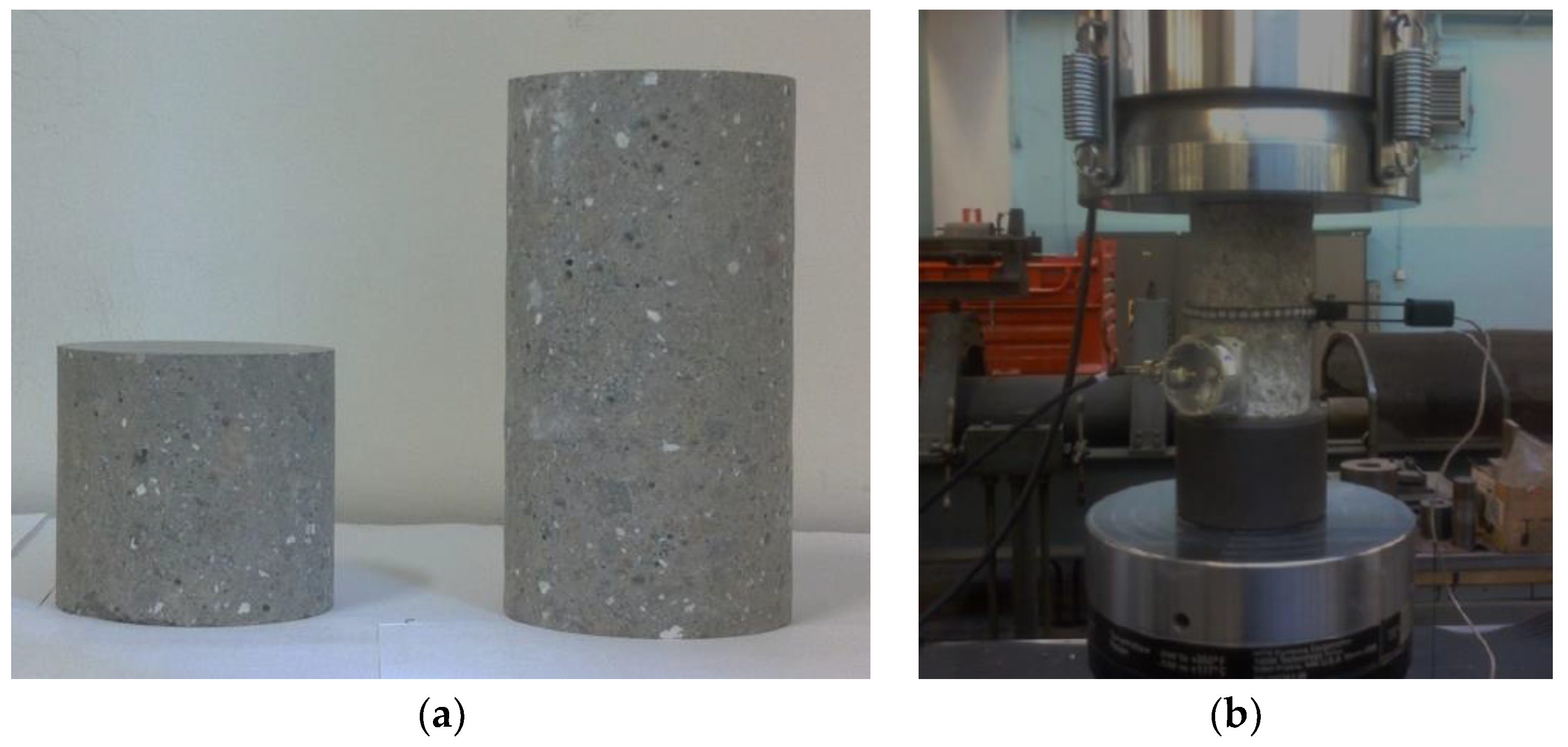
In this section, the results of compression tests performed on concrete specimens having diameter equal to 100 mm, and slenderness λ equal to 1.0 and 2.0 are presented (Figure 1). Generally speaking, in a frictionless condition, for a specimen with slenderness λ ≤ 1.0 a failure mainly governed by crushing is expected, while for a specimen with slenderness λ ≥ 2.0 a failure governed by splitting is taken into account. For intermediate values of slenderness, shear failure is characterized by the formation of inclined slip bands in the bulk of the specimen. For all cases, the cumulated number of AE is strictly correlated to global or local mechanical instabilities in the post-peak regime of the loading process.

The loading process was controlled by the specimen circumferential expansion, measured by means of a linked chain placed around the sample mid-height (Figure 1b). Such a control permitted to fully detect the load-displacement curve, even in case of snap-back phenomena [25,26]. The specimen with a slenderness λ equal to 1.0 was equipped with a thin layer of Teflon in contact between the platen of the testing machine and the specimen ends, to avoid the friction on the bases and facilitate the transversal deformation.

During the compression tests, Acoustic Emission technique was adopted to monitor each specimen. AE signals generating from the fracture phenomena were detected by attaching a piezoelectric sensor to the surface of the specimens with a silicon glue. As stated, the sensor is sensitive in the frequency range (50–800 kHz), and it is placed on the external surface of the monitored samples (Figure 1b). The AE acquisition threshold level was set up to 2 mV, with an amplification gain of the AE signals equal to 60 dB. The recorded waveform sampling frequency was 1 Msample/s.

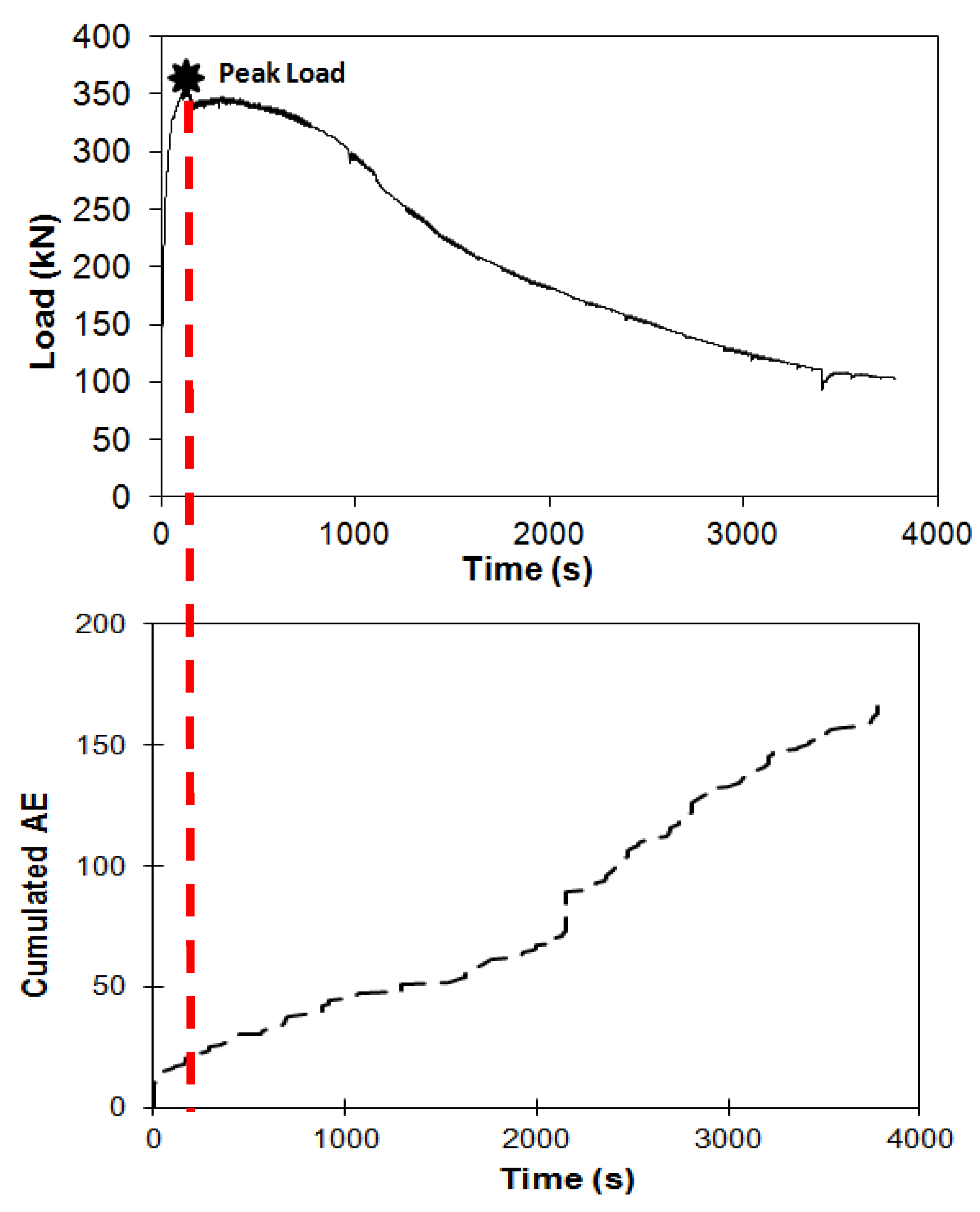
The results obtained from the compression test of specimen with λ = 1.0 are represented in Figure 2, Figure 3 and Figure 4. The signal frequency refers to the average values, the average frequency (AF), which is calculated as the ratio between the AE ring-down counts and the signal duration time, while the energy of each AE signal is calculated according to RILEM [27].

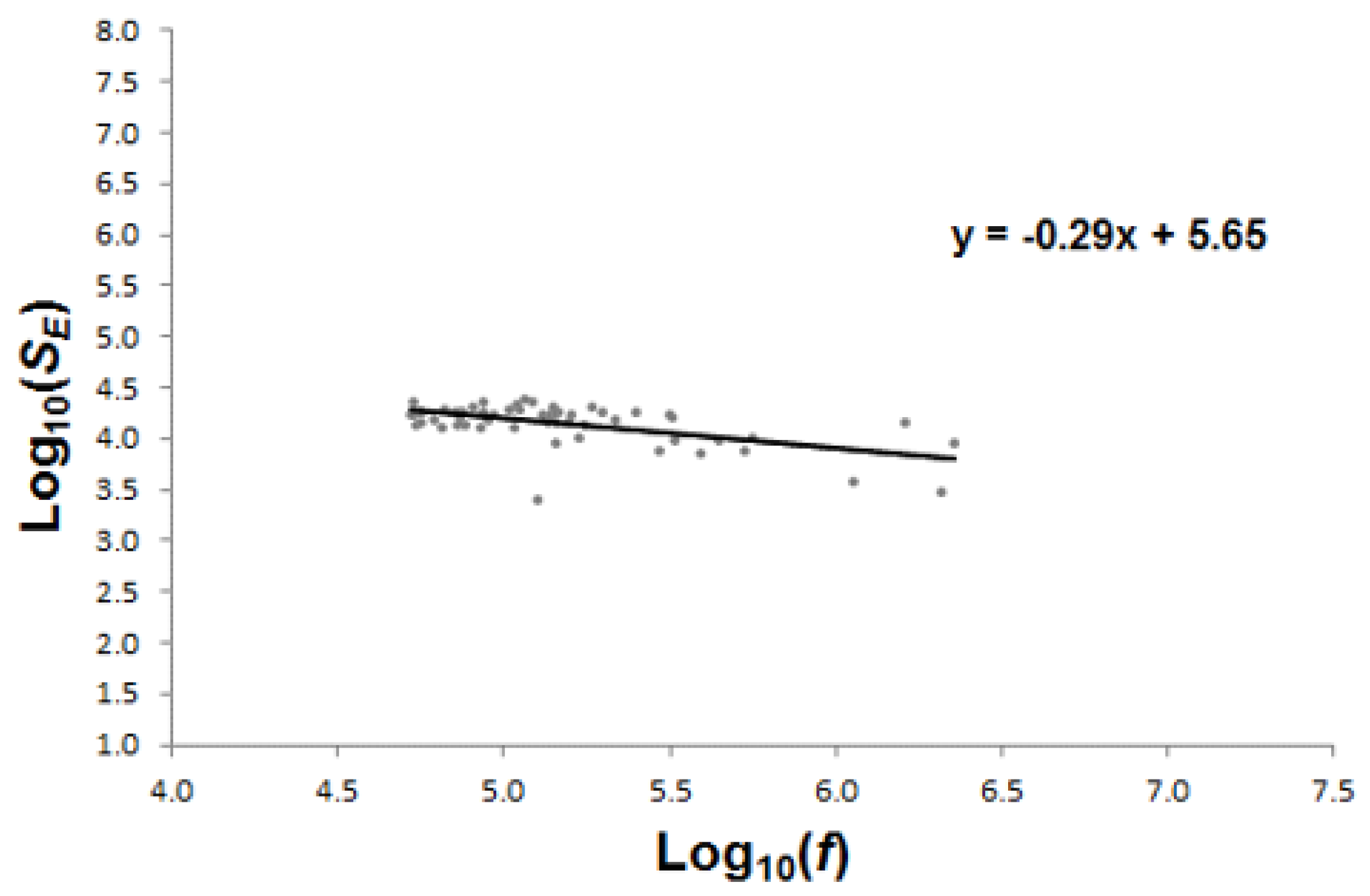
1/f^γ distribution of AE signals is divided into two time windows: before the achievement of the peak load, and after the peak load (Figure 2). In Figure 3, the log-log plot of AE power spectrum versus frequency for signals detected before the peak load is represented. Therefore, a fluctuation of f^-γ (γ ≈ 0.29) is found, which reveals a source noise basically “white” (“white” or random noise: 1/f⁰).

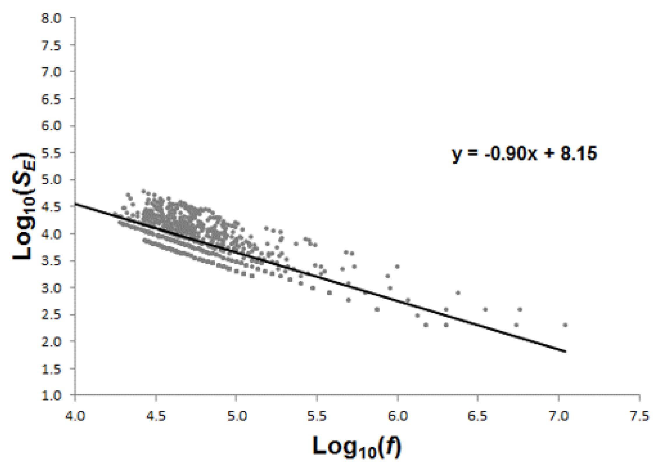
Figure 4 shows the log-log plot of AE power spectrum versus frequency for signals detected after the peak load. For the compression test of the specimen with λ = 1.0 a fluctuation of f^-γ (γ ≈ 0.9) is found, which reveals a source noise basically “pink” (“pink” or correlated noise: γ ~ 1.0 for 1/f^γ).

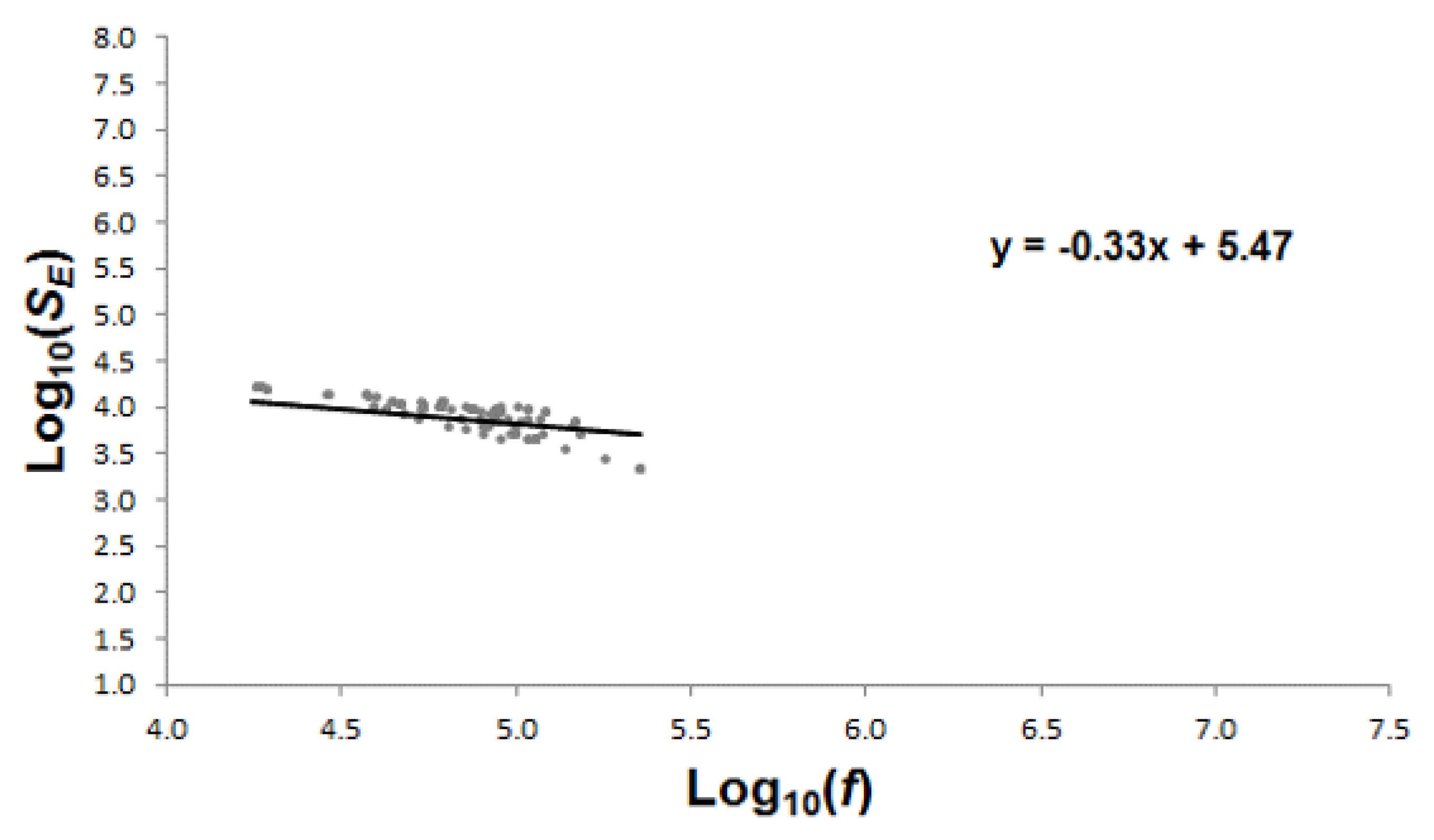
Furthermore, the results obtained from the compression test of specimen with λ = 2.0 are represented in Figure 5, Figure 6 and Figure 7. Also in this case, 1/f^γ distribution of AE signals is divided into two time windows (Figure 5): before the achievement of the peak load, and after peak load. In Figure 6 the log-log plot of AE power spectrum versus frequency for signals detected before the peak load is reported, and a fluctuation of f^-γ (γ ≈ 0.33) is found, which reveals a source noise basically “white” (“white” or random noise: 1/f⁰).

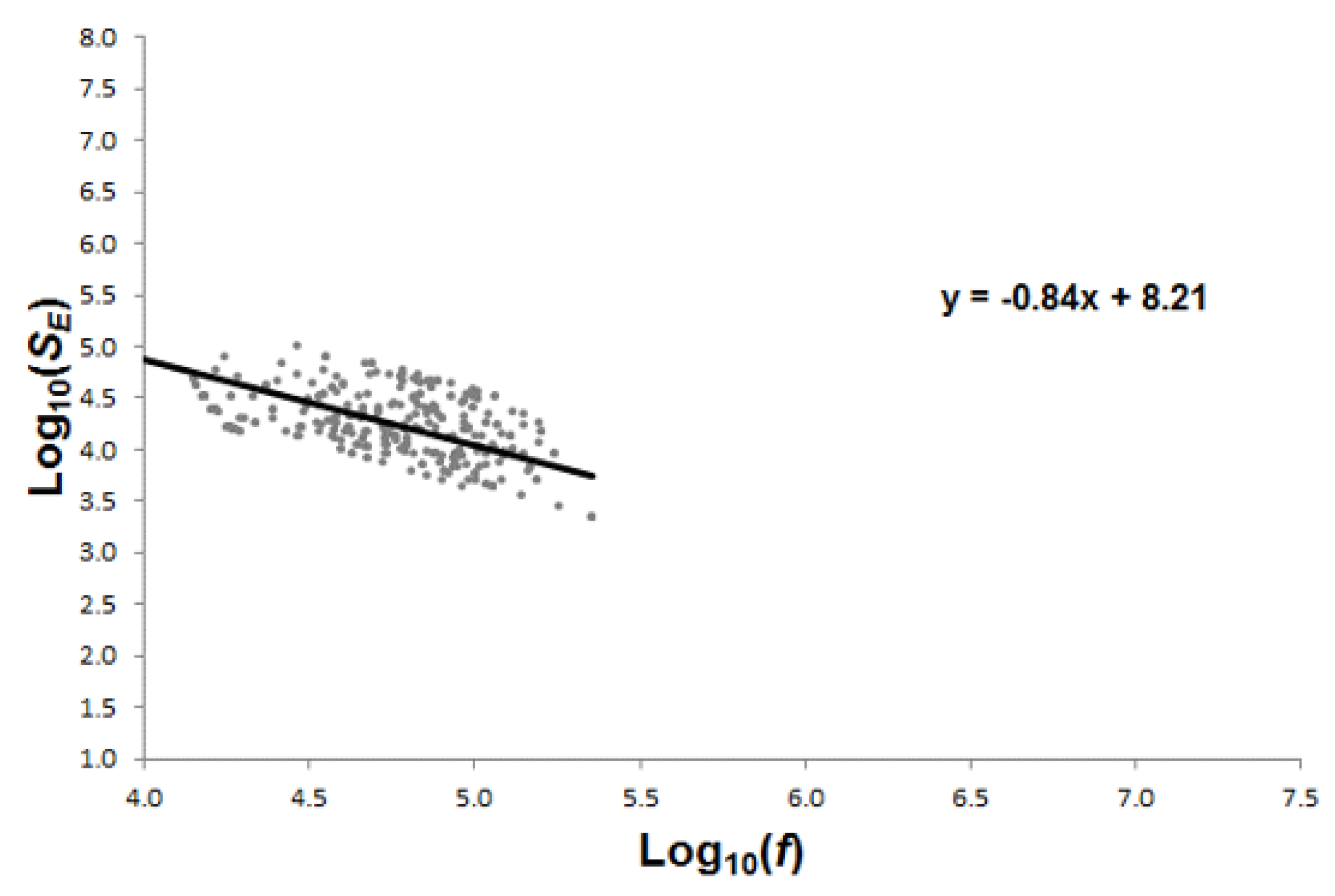
Analogously, in Figure 7 the log-log plot of AE power spectrum versus frequency for signals detected after the peak load is shown. During the compression test of specimen with λ = 2.0 a fluctuation of f^-γ (γ ≈ 0.84) is found, which reveals a source noise basically “pink” (“pink” or correlated noise: 1/f¹).

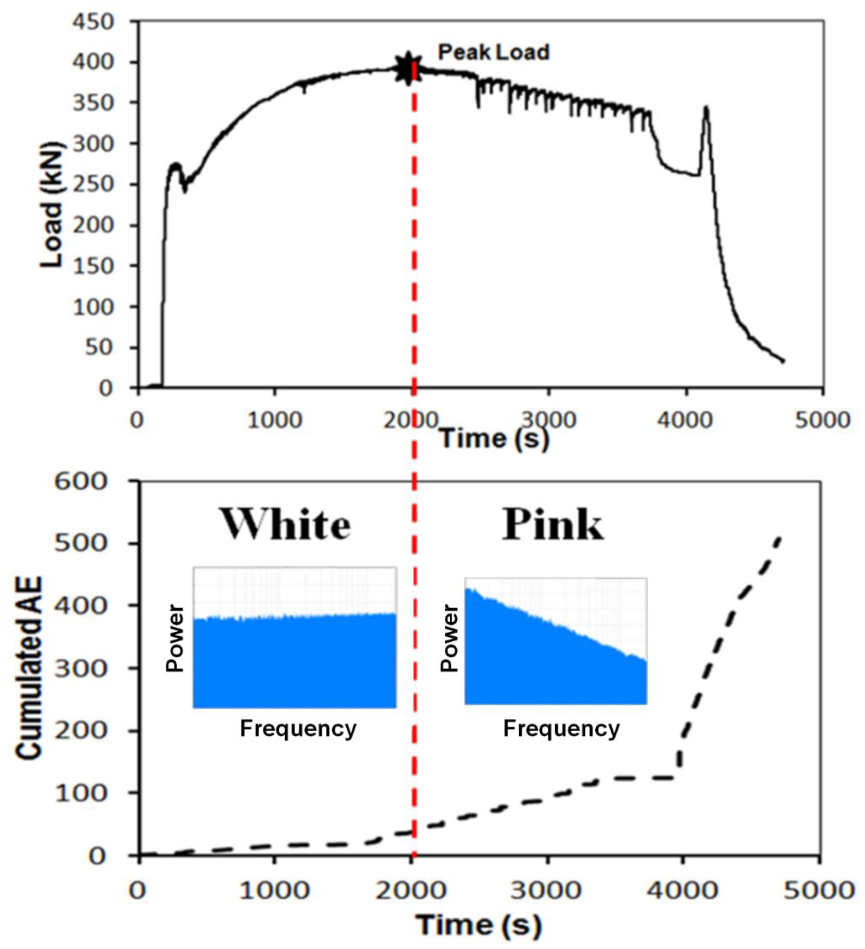
Summarizing, the frequency fluctuation data obtained by the compression tests carried out on concrete cylindrical specimens show how, before the achievement of the peak load, AE signals reveal a source noise basically “white” (1/f⁰) that is characteristic of prominent random phenomena. On the contrary, after peak load, the source noise revealed by AE signal is characterized as “pink” (1/f¹), that is distinctive of correlated phenomena. See, for the sake of synthesis, the graph of Figure 8 that represents the behaviour under compression of the specimen having slenderness 1.

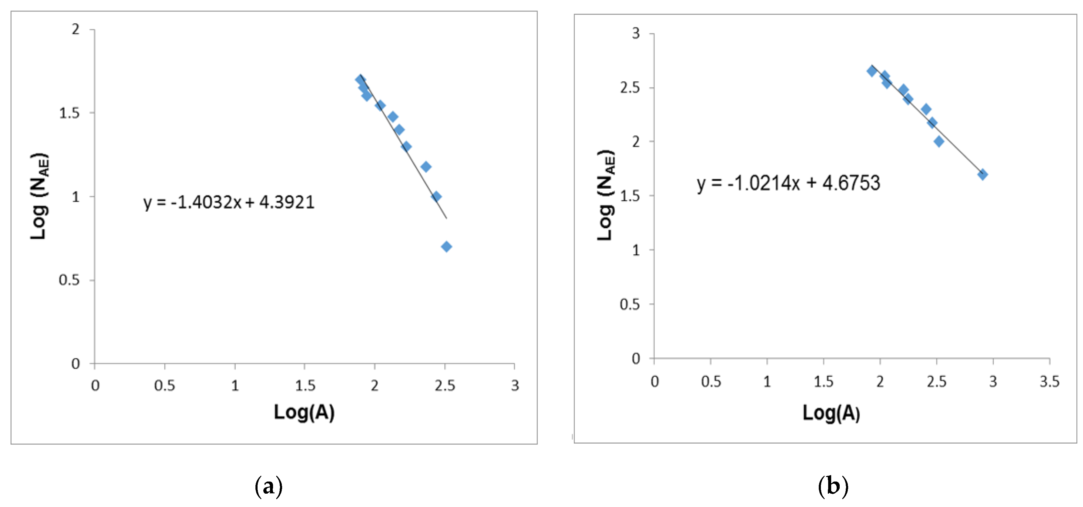
Additionally, b-values of the specimen with λ = 1.0 are reported in Figure 9 both for pre-peak (b ≅ 1.40), and post-peak loading phases (b ≅ 1.02), confirming the 1/f noise as a very suitable indicator of both the critical states and those that precede global or local collapses [25,26]. As a matter of fact, as it is well known in the literature [7,8,9,10,11,12,13,14,15,16,17,18,19,20,21], the statistical interpretation to the variation in the b-value during the evolution of damage detected by AE captures the transition from the condition of diffused criticality to that of imminent failure localization. More precisely, in the pre-peak loading phase of the specimen with λ = 1.0, to the white noise envisaged by the 1/f analysis, corresponds the critical condition also confirmed by the b-value near to 1.5. In this case the energy emission takes place through small defects homogeneously distributed throughout the specimen’s volume. On the contrary, in the post-peak loading phase, to the pink noise envisaged by the 1/f analysis, corresponds a b-value near to 1.0, in this situation the energy emission takes place on preferentially fracture surfaces [9].

3. 1/f Noise in Damaging Structures: In-Situ AE Monitoring

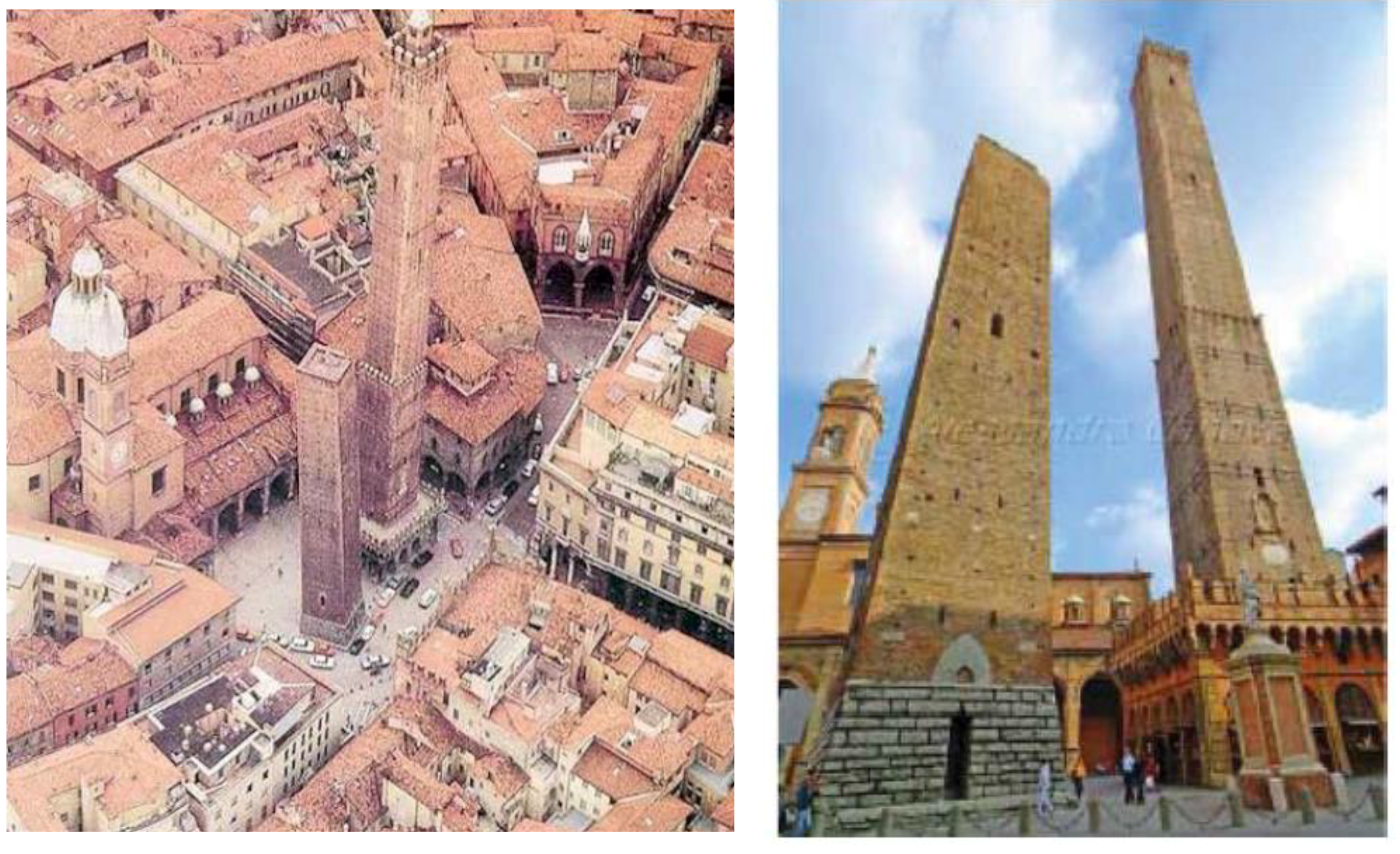
AE technique has been very usefully employed by the authors to investigate on a wide set of structural problems related to ancient masonry buildings [28,29]. In particular, AE technique has been employed to assess the stability of the tallest structure in the city of Bologna (Italy), the Asinelli Tower, which, together with the nearby Garisenda tower, is the renowned symbol of the city (Figure 10) [30]. The Asinelli Tower dates back to the early XII Century, and it is the tallest leaning tower in Italy. The tower measures 97.30 m in height, the side is 8.00 m at the base, and 6.50 m at the top. Its leaning is of 2.38 m westward.

The AE activity was detected in a masonry significant region for monitoring purposes and easy to reach. Six piezoelectric sensors (working in the range of 50–800 kHz) were attacked on the north-east corner of the tower, immediately above the terrace atop the arcade, at an average level of ~9.00 m above ground. In this area, the double-wall masonry has a thickness of ~2.45 m. AE monitoring began on 23 September 2010 at 5:40 p.m., and ended on 28 January 2011 at 1:00 p.m., covering, therefore, a 4-month period. The AE monitoring was carried on exploiting the above mentioned USAM system. To filter out the environmental background noise a detection threshold of 100 mV was settled (appropriate for masonry according to the authors’ experience [28,30]). From the monitoring process carried out on a significant part of this tower, it was possible to evaluate the incidence of seismic activity, vehicle traffic, and wind action on fracture evolution and damaging phenomena within the structure.

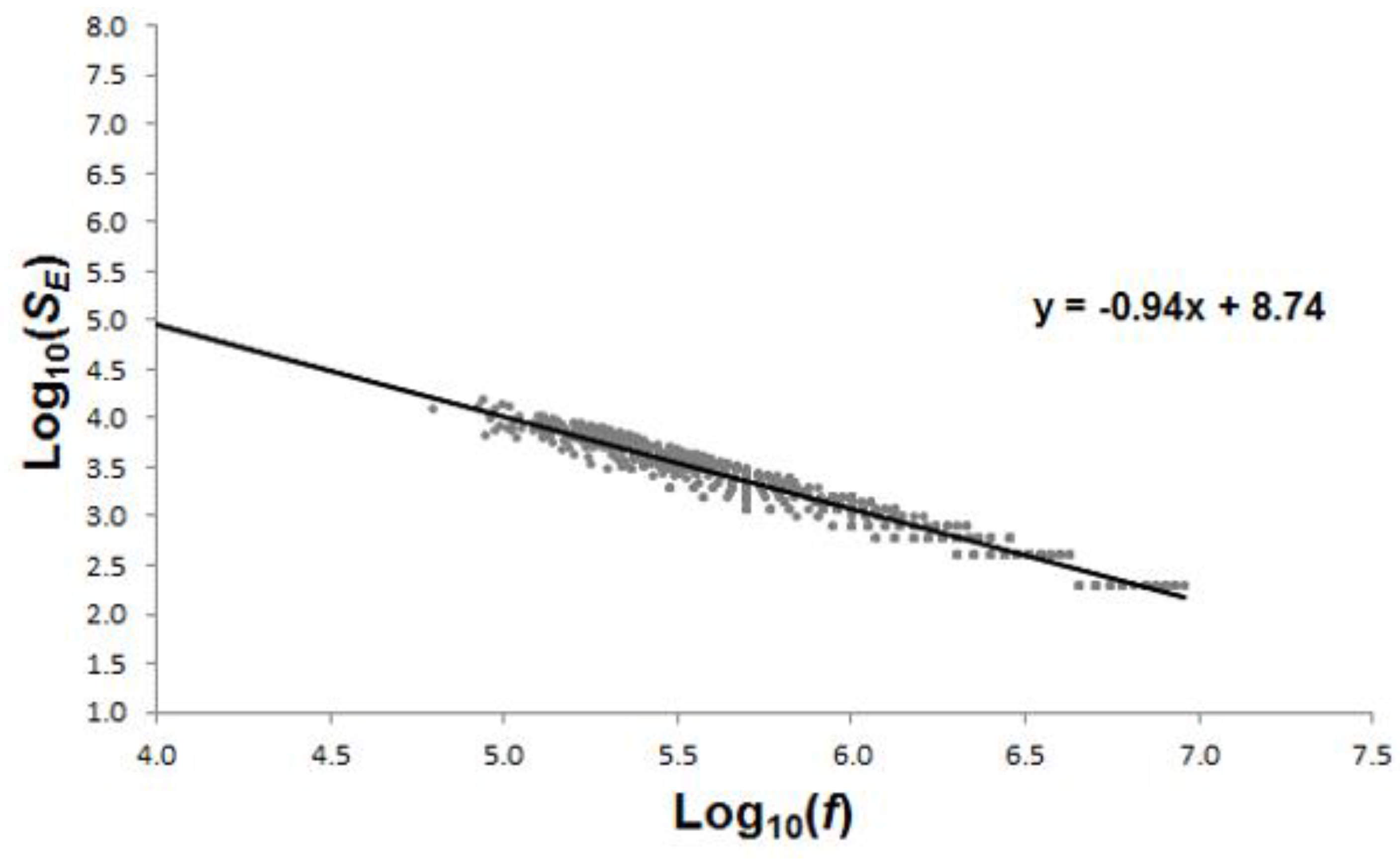
In Figure 11, AE data obtained during the structural monitoring are represented in a log-log plot of power spectrum versus frequency, with a fluctuation of f^-γ (γ = 0.94). Therefore, the source noise revealed by AE signals sounds “pink”, supporting the evidences of the cracking process found during the monitoring campaigns [28,30]. We can say that, in the masonry region monitored by means of AE, pink noise fluctuations suggest that the material strength has been locally overcome, as in the case of the laboratory tests described above.

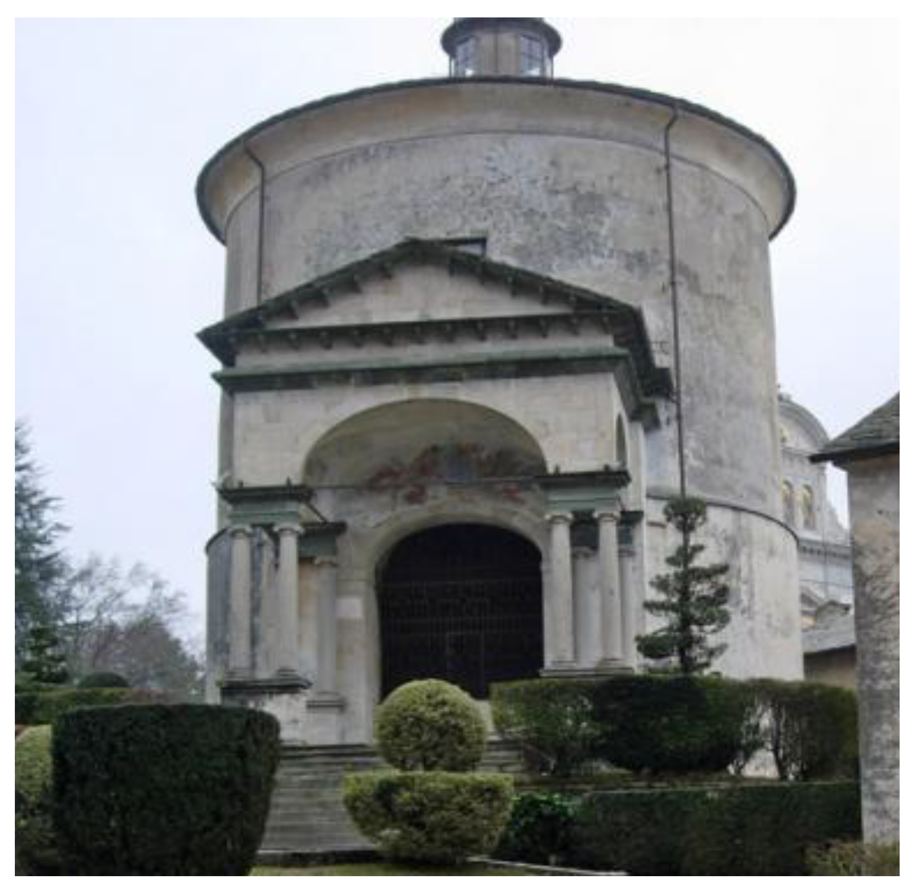
AE technique was successfully applied by the authors, not only to assess historical monument stability, but also to evaluate the structural supports of mural paintings, and the state of conservation of the frescos. As a second object of analysis in this work, the results of the monitoring of Chapel XVII (also known as “The Transfiguration of Christ on Mount Tabor”) of the Sacred Mountain of Varallo is chosen (Figure 12). The most ancient Sacred Mountain of northern Italy is the Sacred Mountain of Varallo, consisting in 45 monumental chapels dating back to the Renaissance period, and it is located at the top of a mount crest, among the green of the forests surrounding the City of Varallo. The chapels contain about 800 multicoloured life-size terracotta statues, representing Life, Passion and Death of Christ [31].

Concerning Chapel XVII structural integrity, a vertical crack of about 3.00 m in length and a detachment of frescos are present, both on the north wall, which are the object of the AE monitoring campaign. AE sensors are employed to monitor the damage evolution of the structural support of the decorated surfaces of Chapel XVII: four are positioned around the vertical crack, while two are positioned near the frescos detachment. For the sensor pasting on valuable decorated surfaces, a suitable methodology is applied [32].

The equipment used for signal acquisition and processing consists of the aforementioned six USAM units. The signals acquisition threshold was settled at 100 μV.

The monitoring period of the structural supports of the chapel began on 28 April 2011 and ended on 4 June 2011, it lasted about 900 h [32]. As results from the monitoring campaign, the vertical crack monitored on the North wall of the chapel presents a distribution of cracks on a surface domain, clearly proved by the b-value in the range (0.95, 1.15). Concerning the monitored frescos detachment, the decorated surface tends to evolve towards metastable conditions, and the acquired signals showed high frequency characteristics (<400 kHz). Moreover, a distribution of microcracks in the volume is obtained for the analyzed region [32].

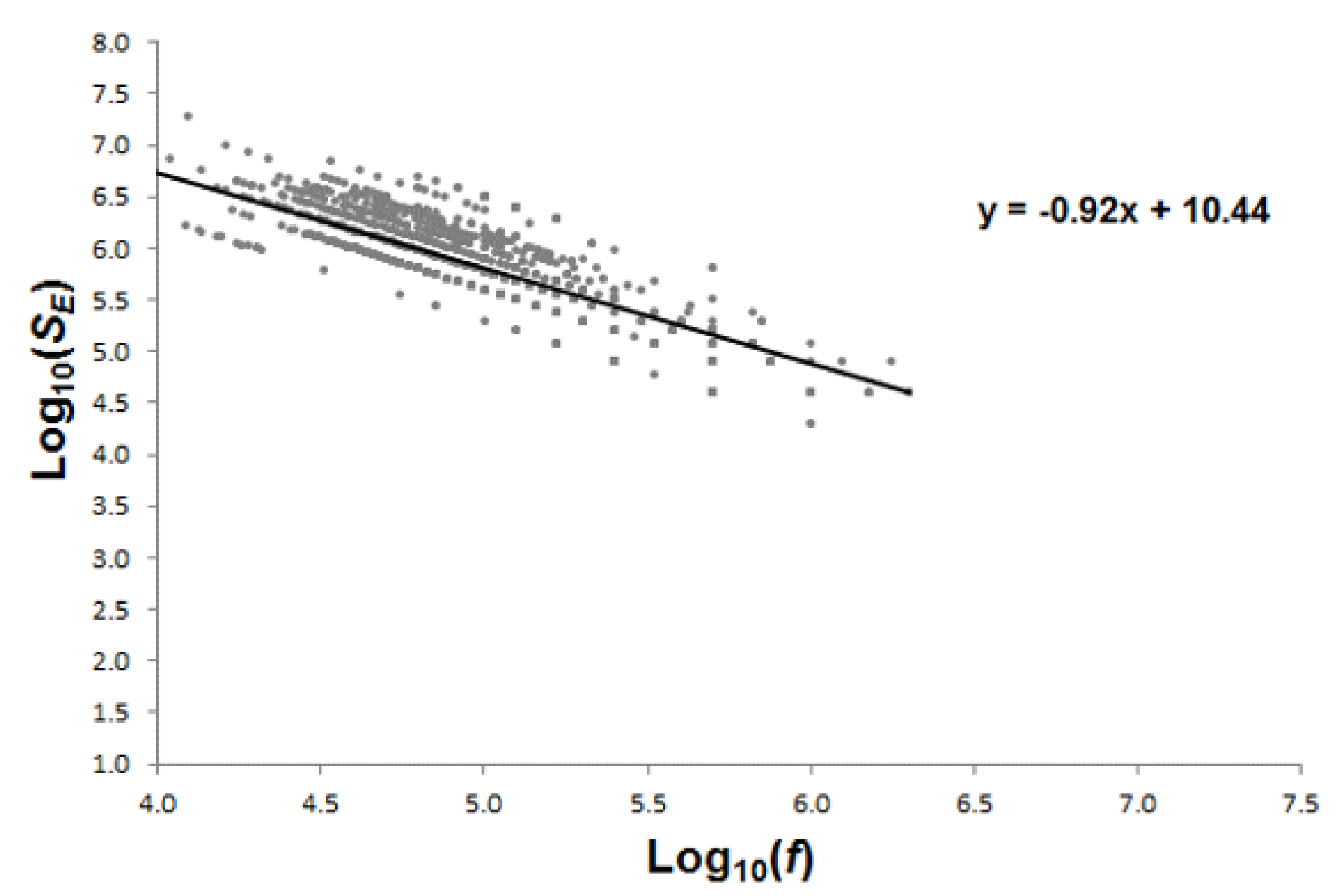
The results obtained by the application of the AE sensors are represented in a log-log plot of power spectrum versus frequency (Figure 13), with a fluctuation of f^-γ (γ = 0.92). Also in this case, the source noise revealed by AE signals sounds “pink”, supporting the evidences of the cracking process found during the monitoring campaigns [24,28,32].

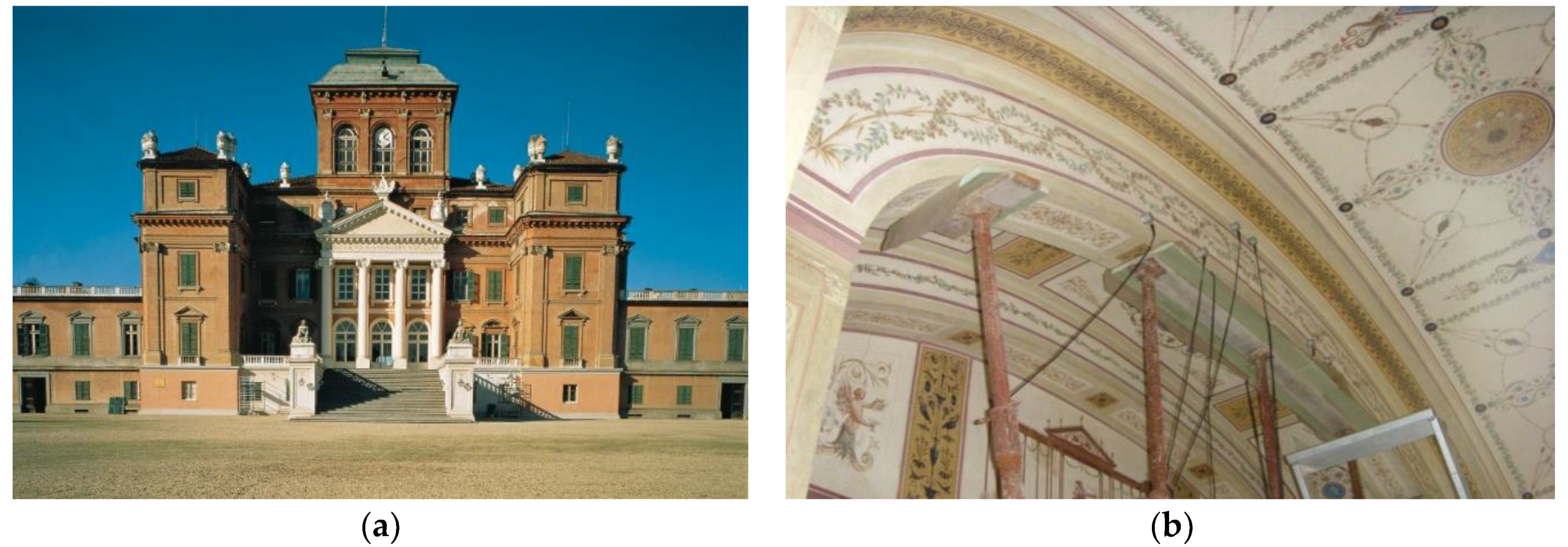
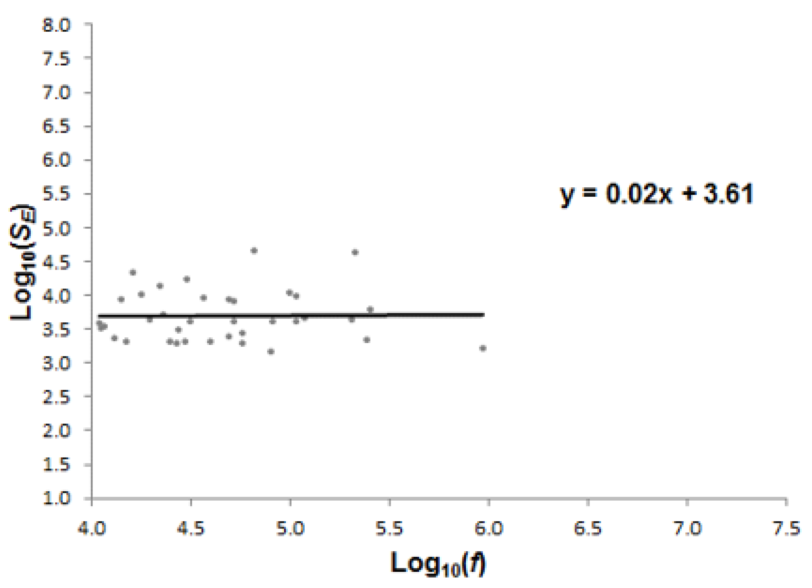
Finally, the log-log plot of the AE power spectrum versus frequency for a monitored masonry arch [33], belonging to the Racconigi Castle (Figure 14a,b) in Piedmont (Italy) is proposed. This last example has been presented in order to demonstrate that a “white” response is obtained on a masonry structural element in which the post-peak loading phase is far from being achieved. From Figure 15, it results 1/f^γ noise with γ ~ 0.0, that characterizes white sources, generated by small defects random diffused in the structural volume.

Comparing the results obtained during the laboratory compression tests, and the data collected from in-situ structural monitoring, we remark a sophistication of the “pink music”, that suggests that 1/f noise may have an essential role in self-organized criticality and correlated processes. By applying it to damage analysis of materials, the distribution 1/f behaves as a very suitable indicator of critical states. At last, recalling the elastic-softening constitutive law for the structural response [26,34], when microcracks are organized on preferential fracture surfaces, the damaging structure “produces” pink noise.

It is possible to find out in the previous discussion a parallel with the statistical distribution analysis of AE events, the so-called b-value [7,8,9,35,36,37,38,39,40]. Therefore, the emitted energy modalities are identified during the monitoring process by determining the b-value variations. b-value extreme cases are: the critical conditions b = 1.5, when the energy emission takes place through small defects diffused homogeneously in the structural volume; and b = 1.0, when energy emission takes place throughout preferential fracture surfaces.

A diffused damage in the former case is observed ($2b=D\simeq 3.0$, i.e., the cracks are distributed in a fractal domain near a volume [41,42,43]), whereas in the latter, two-dimensional macrocracks are formed leading to the separation of the structural element ($2b=D\simeq 2.0$, i.e., the cracks are distributed in a fractal domain close to a surface [41,42,43]). Like the b-value analysis, the proposed 1/f^γ noise model analyzes the transition from the diffused damage condition to that of imminent collapse, when damaging structures sound “pink”.

4. Conclusions

In quasi-brittle materials, like concrete, masonry, and mortar, there is a source of 1/f noise during Acoustic Emissions (AE) from fracture phenomena. The physical origin of 1/f noise is still an open question, and it is interesting to speculate regarding the universality of this particular noise mechanism.

AE data detected from compression tests of concrete specimens with different slenderness, suggest that 1/f^γ noise behaviour is meaningful also in damaging structures.

In fact, before the critical state is reached, it appears 0.29 ≤ γ ≤ 0:33 for 1/f^γ noise. This means that, when the damaging is characterized by the formation of micro-cracks uniformly distributed in the concrete specimen, and the dominant fracture surfaces have not yet been generated, the energy emitted from the material and measured through AE signals, is characterized by small variations for every frequency range. The distribution of micro-cracks in concrete sample is therefore random. As a confirmation, the AE sources appear evenly distributed in the damaged body, $2b=D\simeq 3.0$.

On the other hand, after the critical state, i.e., in the descending branch of the load-time curve, the preferential fracture surfaces are now generated, and the energy emitted by the damaged material is characterized by significant variations in relation to the frequency: the lower the signal frequency, the higher the emitted energy by the damaging body. In this case, the AE sources appear distributed on preferential fracture surfaces, $2b=D\simeq 2.0$.

More precisely, it is interesting to note that, for all the considered cases, during the damage increase, the γ range could be reduced to 0.8 ≤ γ ≤ 0.9 (pink noise).

To highlight this observation, AE data series from in-situ Acoustic Emission monitoring are presented: the first one is referred to the Asinelli Tower, the highest construction in Bologna City center, Italy, built in the early XII Century. The second belongs to the investigation of the state of conservation of the mural paintings and their structural supports in the Chapel XVII of the Sacred Mountain of Varallo Renaissance Complex (Italy). AE data obtained from the two damaging structures show a 1/f^γ-like power spectrum, with a value of γ close to unity (pink noise), suggesting that 1/f noise may behave as a very suitable indicator of both the critical state and that preceding the collapse.

The interpretation of 1/f noise phenomena through the use of the AE technique can be therefore very useful for identifying the transition from the critical conditions of a structure to those that involve an incipient collapse.

References

- Milotti, E. 1/f noise: A pedagogical review. arXiv, 2002; arXiv:physics/0204033. [Google Scholar]
- Mandelbrot, B. Fractals: Form, Chance and Dimension; W. H. Freeman and Company: San Francisco, CA, USA, 1977. [Google Scholar]
- Institute for Telecommunication Sciences—National Telecommunications and Information Administration (ITS-NTIA). Federal Standard 1037C: Glossary of Telecommunication Terms; General Services Administration Information Technology Service: Washington, DC, USA, 1996.
- Dutta, P.; Horn, P.M. Low-frequency fluctuations in solids: 1/f noise. Rev. Mod. Phys. 1981, 53, 497–516. [Google Scholar] [CrossRef]
- Bak, P.; Tang, C.; Wiesenfeld, K. Self-organised criticality: An explanation of 1/f noise. Phys. Rev. Lett. 1987, 59, 381–384. [Google Scholar] [CrossRef] [PubMed]
- Voss, R.F.; Clarke, J. 1/f noise in music and speech. Nature 1975, 258, 317–318. [Google Scholar] [CrossRef]
- Carpinteri, A.; Lacidogna, G.; Pugno, N. Richter’s laws at the laboratory scale interpreted by Acoustic Emission. Mag. Concr. Res. 2006, 58, 619–625. [Google Scholar] [CrossRef]
- Carpinteri, A.; Lacidogna, G.; Puzzi, S. Prediction of cracking evolution in full scale structures by the b-value analysis and Yule statistics. Phys. Mesomech. 2008, 11, 260–271. [Google Scholar] [CrossRef]
- Carpinteri, A.; Lacidogna, G.; Accornero, F.; Mpalaskas, A.C.; Matikas, T.E.; Aggelis, D.G. Influence of damage in the acoustic emission parameters. Cem. Concr. Compos. 2013, 44, 9–16. [Google Scholar] [CrossRef]
- Richter, C.F. Elementary Seismolog; W. H. Freeman and Company: San Francisco, CA, USA; Bailey Bros. & Swinfen Ltd.: London, UK, 1958. [Google Scholar]
- Carpinteri, A.; Lacidogna, G.; Manuello, A. The b-value analysis for the stability investigation of the ancient Athena Temple in Syracuse. Strain 2011, 47, 243–253. [Google Scholar] [CrossRef]
- Aki, A. A Probabilistic Synthesis of Precursory Phenomena. In Earthquake Prediction: An International Review; Simpson, D.W., Richards, P.G., Eds.; American Geophysical Union: Washington, DC, USA, 1981; Volume 4, pp. 566–574. [Google Scholar]
- Main, I.G. A modified Griffith criterion for the evolution of damage with a fractal distribution of crack lengths: Application to seismic event rates and b-values. Geophys. J. Int. 1991, 107, 353–362. [Google Scholar] [CrossRef]
- Main, I.G. Damage mechanics with long-range interactions: Correlation between the seismic b-value and the two point correlation dimension. Geophys. J. Int. 1992, 111, 531–541. [Google Scholar] [CrossRef]
- Main, I.G. A damage mechanics model for power-law creep and earthquake aftershock and foreshock sequences. Geophys. J. Int. 2000, 142, 151–161. [Google Scholar] [CrossRef] [Green Version]
- Carpinteri, A.; Lacidogna, G.; Niccolini, G. Fractal analysis of damage detected in concrete structural elements under loading. Chaos Solitons Fractals 2009, 42, 2047–2056. [Google Scholar] [CrossRef]
- Carpinteri, A.; Lacidogna, G.; Puzzi, S. From criticality to final collapse: Evolution of the b-value from 1.5 to 1.0. Chaos Solitons Fractals 2009, 41, 843–853. [Google Scholar] [CrossRef]
- King, G.C.P. The accommodation of large strains in the upper lithosphere of the earth and other solids by self-similar fault systems: The geometrical origin of b-value. Pure Appl. Geophys. 1983, 121, 761–815. [Google Scholar] [CrossRef]
- Hirata, T. A correlation between b-value and the fractal dimension of earthquakes. J. Geophys. Res. 1989, 94, 7507–7514. [Google Scholar] [CrossRef]
- Rundle, J.B.; Turcotte, D.L.; Shcherbakov, R.; Klein, W.; Sammis, C. Statistical physics approach to understanding the multiscale dynamics of earthquake fault systems. Rev. Geophys. 2003, 41, 1–30. [Google Scholar] [CrossRef]
- Turcotte, D.L. Fractals and Chaos in Geology and Geophysic; Cambridge University Press: New York, NY, USA, 1997. [Google Scholar]
- Aggelis, D.G. Wave propagation through engineering materials; Assessment and monitoring of structures through non-destructive techniques. Mater. Struct. 2013, 146, 519–532. [Google Scholar] [CrossRef]
- Livitsanos, G.; Shetty, N.; Hündgen, D.; Verstrynge, E.; Wevers, M.; Van Hemelrijck, D.; Aggelis, D.G. Acoustic emission characteristics of fracture modes in masonry materials. Constr. Build. Mater. 2018, 162, 914–922. [Google Scholar] [CrossRef]
- Carpinteri, A.; Lacidogna, G.; Invernizzi, S.; Accornero, F. The Sacred Mountain of Varallo in Italy: Seismic risk assessment by Acoustic Emission and structural numerical models. Sci. World J. 2013, 2013, 170291. [Google Scholar] [CrossRef] [PubMed]
- Carpinteri, A.; Corrado, M.; Lacidogna, G. Heterogeneous materials in compression: Correlations between absorbed, released and acoustic emission energies. Eng. Fail. Anal. 2013, 33, 236–250. [Google Scholar] [CrossRef]
- Carpinteri, A.; Accornero, F. Multiple snap-back instabilities in progressive microcracking coalescence. Eng. Fract. Mech. 2018, 187, 272–281. [Google Scholar] [CrossRef]
- RILEM Technical Committee (Masayasu Ohtsu). Recommendation of RILEM TC212-ACD: Acoustic Emission and related NDE techniques for crack detection and damage evaluation in concrete: Measurement method for acoustic emission signals in concrete. Mater. Struct. 2010, 43, 1177–1181. [Google Scholar] [CrossRef]
- Lacidogna, G.; Accornero, F.; Carpinteri, A. Masonry structures. In Innovative AE and NDT Techniques for On-Site Measurement of Concrete and Masonry Structures (RILEM); Ohtsu, M., Ed.; Springer: Heidelberg, Germany, 2016; Chapter 3; pp. 27–46. [Google Scholar]
- Lacidogna, G.; Manuello, A.; Niccolini, G.; Accornero, F.; Carpinteri, A. Acoustic Emission Wireless Monitoring of Structures. In Acoustic Emission and Related Non-Destructive Evaluation Techniques in the Fracture Mechanics of Concrete; Ohtsu, M., Ed.; Woodhead Publishing: Cambridge, UK, 2015; Chapter 2; pp. 15–40. [Google Scholar]
- Carpinteri, A.; Lacidogna, G.; Manuello, A.; Niccolini, G. A study on the structural stability of the Asinelli Tower in Bologna. Struct. Control Health Monit. 2016, 23, 659–667. [Google Scholar] [CrossRef]
- Niccolini, G.; Borla, O.; Accornero, F.; Lacidogna, G.; Carpinteri, A. Scaling in damage by electrical resistance measurements: An application to the terracotta statues of the Sacred Mountain of Varallo Renaissance Complex (Italy). Rend. Lincei—Sci. Fis. Nat. 2014, 26, 203–209. [Google Scholar] [CrossRef]
- Accornero, F.; Invernizzi, S.; Lacidogna, G.; Carpinteri, A. The Sacred Mountain of Varallo renaissance complex in Italy: Damage analysis of decorated surfaces and structural supports. In Acoustic, Electromagnetic, Neutron Emissions from Fracture and Earthquakes; Carpinteri, A., Lacidogna, G., Manuello, A., Eds.; Springer: Heidelberg, Germany, 2015; Chapter 17; pp. 249–264. [Google Scholar]
- Niccolini, G.; Manuello, A.; Marchis, E.; Carpinteri, A. Signal frequency distribution and natural-time analyses from acoustic emission monitoring of an arched structure in the Castle of Racconigi. Nat. Hazards Earth Syst. Sci. 2017, 17, 1025–1032. [Google Scholar] [CrossRef] [Green Version]
- Lacidogna, G.; Accornero, F. Elastic, plastic, fracture analysis of masonry arches: A multi-span bridge case study. Curved Layer Struct. 2018, 5, 1–9. [Google Scholar] [CrossRef] [Green Version]
- Kurz, J.H.; Finck, F.; Grosse, C.U.; Reinhardt, H.W. Stress drop and stress redistribution in concrete quantified over time by the b-value analysis. Struct. Health Monit. 2006, 5, 69–81. [Google Scholar] [CrossRef]
- Shiotani, T.; Fujii, K.; Aoki, T.; Amou, K. Evaluation of Progressive Failure using AE Sources and Improved b-value on Slope Model Tests. Prog. Acoust. Emiss. 1994, 7, 529–534. [Google Scholar]
- Scholz, C.H. The frequency-magnitude relation of microfracturing in rock and its relation to earthquakes. Bull. Seismol. Soc. Am. 1968, 58, 399–415. [Google Scholar]
- Colombo, S.; Main, I.G.; Forde, M.C. Assessing damage of reinforced concrete beam using “b-value” analysis of acoustic emission signals. J. Mater. Civ. Eng. ASCE 2003, 15, 280–286. [Google Scholar] [CrossRef]
- Rao, M.V.M.S.; Prasanna Lakshmi, K.J. Analysis of b-value and improved b-value of acoustic emissions accompanying rock fracture. Curr. Sci. 2005, 89, 1577–1582. [Google Scholar]
- Lockner, D.A.; Byerlee, J.D.; Kuksenko, V.; Ponomarev, A.; Sidorin, A. Quasi static fault growth and shear fracture energy in granite. Nature 1991, 350, 39–42. [Google Scholar] [CrossRef]
- Lacidogna, G.; Accornero, F.; Carpinteri, A. Influence of snap-back instabilities on Acoustic Emission damage monitoring. Eng. Fract. Mech. 2018. [Google Scholar] [CrossRef]
- Carpinteri, A.; Corrado, M.; Lacidogna, G. Three different approaches for damage domain characterization in disordered materials: Fractal energy density, b-value statistics, renormalization group theory. Mech. Mater. 2012, 53, 15–28. [Google Scholar] [CrossRef]
- Carpinteri, A.; Lacidogna, G.; Niccolini, G.; Puzzi, S. Morphological fractal dimension versus power-law exponent in the scaling of damaged media. Int. J. Damage Mech. 2009, 18, 259–282. [Google Scholar] [CrossRef]
Figure 1.
Concrete specimens subjected to compression test monitored by means of Acoustic Emission (a); Experimental set-up (b).
Figure 2.
Concrete specimen with λ = 1: Load vs. time diagram; Cumulated AE (hits) versus time diagram. Red line refers to the peak load occurrence.
Figure 3.
Log-log plot of AE power spectrum versus frequency for the concrete specimen (λ = 1): 1/fγ noise before peak load, with γ = 0.29. White noise source (Random phenomena).
Figure 4.
Log-log plot of AE power spectrum versus frequency for the concrete specimen (λ = 1): 1/fγ noise after peak load, with γ = 0.90. Pink noise source (Correlated phenomena).
Figure 5.
Concrete specimen with λ = 2: Load vs. time diagram; Cumulated AE (hits) versus time diagram. Red line refers to the peak load occurrence.
Figure 6.
Log-log plot of AE power spectrum versus frequency for the concrete specimen (λ = 2): 1/fγ noise before peak load, with γ = 0.33. White noise source (Random phenomena).
Figure 7.
Log-log plot of AE power spectrum versus frequency for the concrete specimen (λ = 2): 1/fγ noise after peak load, with γ = 0.84. Pink noise source (Correlated phenomena).
Figure 8.
Concrete specimen (λ = 1) subjected to compression test: Load vs. time diagram; Cumulated AE versus time diagram with signal frequency fluctuations (qualitative trend). Red line refers to the peak load occurrence.
Figure 9.
Concrete specimen (λ = 1.0) subjected to compression test: b-value for pre-peak loading phase (a); b-value for post-peak loading phase (b).
Figure 10.
The Garisenda Tower and the Asinelli Tower, in Bologna City center.
Figure 11.
Log-log plot of AE power spectrum versus frequency for the Asinelli Tower, Bologna: 1/fγ noise, with γ = 0.94. Pink noise source (Correlated phenomena).
Figure 12.
External view of Chapel XVII of the Sacred Mountain of Varallo (Italy).
Figure 13.
Log-log plot of AE power spectrum versus frequency for the Chapel XVII of the Sacred Mountain of Varallo: 1/fγ noise, with γ = 0.92. Pink noise source (Correlated phenomena).
Figure 14.
External view of the Racconigi Castle (Italy) (a) and the monitored masonry arch inside the Castle (b).
Figure 15.
Log-log plot of AE power spectrum versus frequency for the monitored masonry arch: 1/fγ noise, with γ ~ 0.0. White noise source (Random phenomena).
© 2018 by the authors. Licensee MDPI, Basel, Switzerland. This article is an open access article distributed under the terms and conditions of the Creative Commons Attribution (CC BY) license (http://creativecommons.org/licenses/by/4.0/).
Share and Cite
MDPI and ACS Style
Carpinteri, A.; Lacidogna, G.; Accornero, F. Fluctuations of 1/f Noise in Damaging Structures Analyzed by Acoustic Emission. Appl. Sci. 2018, 8, 1685. https://doi.org/10.3390/app8091685
AMA Style
Carpinteri A, Lacidogna G, Accornero F. Fluctuations of 1/f Noise in Damaging Structures Analyzed by Acoustic Emission. Applied Sciences. 2018; 8(9):1685. https://doi.org/10.3390/app8091685
Chicago/Turabian StyleCarpinteri, Alberto, Giuseppe Lacidogna, and Federico Accornero. 2018. "Fluctuations of 1/f Noise in Damaging Structures Analyzed by Acoustic Emission" Applied Sciences 8, no. 9: 1685. https://doi.org/10.3390/app8091685
Note that from the first issue of 2016, this journal uses article numbers instead of page numbers. See further details here.