Assessment of Turbulence Modelling in the Wake of an Actuator Disk with a Decaying Turbulence Inflow

Abstract

The characteristics of the turbulence field in the wake produced by a wind turbine model are studied. To this aim, a methodology is developed and applied to replicate wake measurements obtained in a decaying homogeneous turbulence inflow produced by a wind tunnel. In this method, a synthetic turbulence field is generated to be employed as an inflow of Large-Eddy Simulations performed to model the flow development of the decaying turbulence as well as the wake flow behind an actuator disk. The implementation is carried out on the OpenFOAM platform, resembling a well-documented procedure used for wake flow simulations. The proposed methodology is validated by comparing with experimental results, for two levels of turbulence at inflow and disks with two different porosities. It is found that mean velocities and turbulent kinetic energy behind the disk are well estimated. The development of turbulence lengthscales behind the disk resembles what is observed in the free flow, predicting the ambient turbulence lengthscales to dominate across the wake, with little effect of shear from the wake envelope. However, observations of the power spectra confirm that shear yields a boost to the turbulence energy within the wake noticeable only in the low turbulence case. The results obtained show that the present implementation can successfully be used in the modelling and analysis of turbulence in wake flows.

1. Introduction

Studies of turbulence in the wake of wind turbines are often made with the aim of analyzing the influence of the flow and rotor models in the reproduction of wake characteristics. Investigations with various rotor models in the Atmospheric Boundary Layer (ABL) have been made either with the goal of improving the production efficiency of a cluster of turbines (e.g., [1,2,3,4]) or aimed at comparing the characteristics of wakes with respect to measurements of real or downscaled turbines (e.g., [5,6,7,8]). When numerical simulations of large wind parks are made, computational limitations oblige employing simpler rotor models that, while numerically less expensive, are requested to produce a minimum level of detail in wake features that yields an acceptable reproduction of the interaction of the ensuing wakes and the downstream wind turbines, as well as other wakes. Amongst the simplest formulations of the rotor model is the Actuator Disk (AD) [9,10] which reproduces the effect of the rotor in the incoming flow by means of a permeable surface in the shape of a disk that acts as a momentum sink. In its most basic conception, the AD constitutes a one-dimensional force opposite to the flow, perpendicular to the rotor plane, with no wake rotation or airfoil properties considered. Different studies [8,11,12] have shown the capability of the AD technique to approximate the characteristics of a real turbine wake within its far region. An experimental investigation of the wakes produced by porous disks has been performed by [13,14], where the disks are made of metallic meshes representing different solidities. In recent work, similar research has been made of wakes produced by a decaying turbulence inflow [15,16]. Unlike the ABL, no shear-produced turbulence occurs, greatly simplifying the modelling of the flow physics and permitting to isolate the features of the wake from those deriving from the inflow (e.g., the vertical momentum flux in the ABL). With data collected in a related measurement campaign, the authors of [17] employed Reynolds-Averaged Navier–Stokes (RANS) models to reproduce measurements in the wakes produced by the porous disks. Although good results are obtained, the experimental study represents an opportunity to perform comparisons with numerical simulations that allow a greater detail in the reproduction of the turbulence characteristics. Therefore, the reproduction of these experiments employing Large-Eddy Simulations (LES) seems appealing.

To reproduce the inflow properties measured experimentally, first it is necessary to model the flow of decaying turbulence produced in a wind tunnel. In this regard, different works have been dedicated to investigate various methodologies to produce adequate inlet conditions [18,19,20]. Amongst the different techniques, the method developed by Mann [21,22,23] to create a synthetic turbulence field has often been used to create inflow conditions for simulations in ABL [5,6,24,25] as well as in homogeneous turbulence [26,27,28]. In these works, it has been shown that the Mann method is capable of producing realistic turbulence fields, resembling the second order statistics of real turbulence [5,29]. This algorithm permits creating synthetic fields of homogeneous turbulence by prescribing two parameters, the turbulence lengthscale and (albeit indirectly) the turbulence intensity. An anisotropy factor is also used in the algorithm to create boundary layer fields. The transition and evolution of turbulence characteristics when synthetic fields are introduced in LES domains, especially of integral lengthscales, has been previously studied by [27] for homogeneous turbulence and recently by [24,30] (using the turbulence generation method of [20]) in sheared flows.

The objective of this work is the study of turbulence characteristics in the wake flow of a wind turbine model. To fulfill this purpose, a methodology is developed to replicate: (1) the turbulence characteristics of a homogeneous wind tunnel flow and (2) the wake field arising from the introduction of porous disks representing the wind turbine. This procedure is employed to reproduce the inflow and wake characteristics measured in the experimental campaign carried out by G. Espana and S. Aubrun [17,31], so the comparison with wind tunnel data serves as method of validation. The study of diverse features of the turbulence field both in the free decaying flow and in the wake is presented next to such comparison. The computational platform employed is OpenFOAM^® v.2.1 [32,33] (the OpenFOAM Foundation Ltd., London, UK) an open-source code amply used in flow simulations, chosen for its availability and access to apply ad-hoc modifications to existing solvers and utilities. While the synthetic turbulence is created with the Mann method, the flow is reproduced using LES computations. The methodology implemented follows—in part—a procedure developed on the CFD software EllipSys3D [34,35,36] (Department of Mechanical Engineering and RisøCampus, DTU, Lyngby, Denmark) to simulate wake flows with turbulent inflows [5]. It has been shown that this method provides good results to introduce ABL as well as homogeneous turbulence conditions [5,6,24,25,26,27,28]. By using this approach, we expect to assess: (a) how well the main turbulence characteristics can be reproduced (e.g., turbulence intensity and integral lengthscale) in the inflow and in the wake with LES, (b) how the main turbulence characteristics in the wind tunnel change due to the presence of the wind turbine model and (c) how the LES modelling change along the wake compared to the undisturbed flow (resolved/modelled velocity fluctuations). It should be noted that these questions are formulated in the context of a limited mesh resolution, which makes it more relevant for the wind energy field since it is often desired to minimize the computational requirements while successfully reproducing the requested flow features, which in this case consists mainly of the integral lengthscale.

The work presented here is organized as follows: a brief theoretical background is provided about the homogenenous isotropic turbulence and its experimental approximation, the decaying homogeneous turbulence, next to a description of the measurement campaign and data to be reproduced. Later, the methodology is described in detail, with special attention to the generation of turbulence inflow and the reproduction of the adequate characteristics in the absence of disk. This also comprises the description of the methodology employed to introduce the synthetic turbulence in the LES domain. Next, the results are presented and discussed for the different quantities computed in the turbulence field of the wakes. A final section presents a summary and the conclusions of the work.

2. Homogeneous Turbulence

For a given flow, the instantaneous velocity vector is referred to as $u_i$ whose components in the streamwise, vertical and spanwise directions $(x,y,z)$ are $u_i=(u,v,w)$. The Reynolds decomposition in the streamwise direction is defined as $u=〈U〉+u^{\prime }$, where “$〈·〉$” denotes time-average (capital letters are also used to emphasize averaged magnitudes). The characteristic size of the largest eddies is identified as the distance L required to nullify the correlation function ${\mathcal{R}}_{ij}(\mathbf{r},t)$. With this assumption, the integral lengthscale

$$L_{ij}^{\left(d\right)}={\int }_0^{\infty }{\mathcal{R}}_{ij}({\mathrm{e}}_{d}r,t)dr$$

(1)

in the direction d (set by the unitary vector $\mathrm{e}$) is defined [37]. From all scales defined by this expression, those most commonly used are the longitudinal integral lengthscale $L_1=L_{11}^{\left(1\right)}$ as well as the transversal one $L_2=L_{22}^{\left(1\right)}$. Similarly, the longitudinal Taylor lengthscale (or micro-scale) ${\lambda }_1={\lambda }_{11}^{\left(1\right)}$ is defined by the osculating parabola to the correlation function ${\mathcal{R}}_{ij}(\mathbf{r},t)$. If isotropy is assumed (or at least between the 1 and 2 directions) the equivalences $L_{22}^{\left(1\right)}=L_{11}^{\left(2\right)}$ and ${\lambda }_{22}^{\left(1\right)}={\lambda }_{11}^{\left(2\right)}$ are also valid.

In the absence of shear, the Taylor hypothesis of frozen turbulence can be adopted more comfortably. This is, it is assumed that the turbulence field does not change as it is convected by the mean wind at $〈U〉$, which yields the equivalence between the spatial and temporal correlations. In this way, correlations can be made from the time series of each velocity component. In particular, the autocorrelation will provide the integral time scales ${\mathcal{T}}_{11}$ and ${\mathcal{T}}_{22}$ from where the integral lengthscales can be computed by means of $L_1=〈U〉{\mathcal{T}}_{11}$ and $L_2=〈U〉{\mathcal{T}}_{22}$. Likewise, the longitudinal Taylor lengthscale can be calculated from the expression

$$\frac{1}{{\lambda }_1^2}=\frac{{〈U〉}^{-2}}{2〈{u_1^{\prime }}^2〉}〈{\left(\frac{\partial u_1^{\prime }}{\partial t}\right)}^2〉$$

(2)

as seen in [38] (note that Equation (2) differs from the one presented in that report by a factor of $\sqrt{2}$). Considering the turbulent kinetic energy of a field $k=\frac{1}{2}\left(〈u_1^{\prime 2}〉+〈v_2^{\prime 2}〉+〈w_3^{\prime 2}〉\right)$ and the assumption of isotropy, ${\lambda }_2$ is related to the amount of dissipation of k by

$$\epsilon =\frac{15\nu 〈{u_1^{\prime }}^2〉}{{\lambda }_2^2}=\frac{30\nu 〈{u_1^{\prime }}^2〉}{{\lambda }_1^2}.$$

(3)

When grid turbulence is used to approximate the theoretical case of decaying isotropic turbulence, the characteristics observed at different positions downstream from the grid correspond to the time evolution of isotropic turbulence with zero mean velocity. Thus, a decay during the interval $\Delta t$ is approximated by that occurring within $\Delta x$ in a wind tunnel. In this manner, it has been observed that the decay of k follows the expression

$$\frac{k}{{〈U〉}^2}=c_A{\left(\frac{x-x_0}{M}\right)}^{-n},$$

(4)

where M is the turbulence grid size, $c_A$ (also written as $1/A$) is a fitting parameter, n is the decay exponent and $x_0$ a virtual origin. Equation (4) is commonly employed to track the streamwise turbulence intensity decay, replacing k for $〈{u_1^{\prime }}^2〉$. While Ref. [37] mentions $1.1\le n\le 1.3$ and $c_A\simeq 1/30$, Ref. [39] reports to have observed $n=1.25$ with $x_0=0$, whereas Ref. [40] mentions $1.15\le n\le 1.45$, remarking that $c_A$ varies greatly depending on the geometry of the grid and Re_λ. Ref. [37] indicates that the integral lengthscale evolves downstream according to

$$L_2\simeq c_{B_1}M{\left[\frac{x-x_0}{M}\right]}^{n_1}$$

(5)

with $c_{B_1}=0.06$ and $n_1=0.35$.

3. Experimental Setup and Measurement Campaigns

The measurements used in this work come from experiments performed in the Eiffel-type wind tunnel of the Prisme laboratory of the University of Orléans. The test section has a width and a height of 0.5 m and a length of 2 m. Two different grids were used to generate turbulence at the entrance of the test section, resulting in two different turbulence intensities. At a distance of $x=0.5$ m from that grid, the reported values of turbulence intensity and integral lengthscale (measured at the centreline) were $\mathrm{TI}=3\%$ and $L_1=0.01$ m as well as $\mathrm{TI}=12\%$ and $L_1=0.03$ m. These two inflow cases are henceforward identified as Ti3 and Ti12, respectively. The streamwise position where these values are reported is referred to as the target position $x_D$.

Later, disks made of a metallic mesh were located at $x_D$ to simulate the effect of the AD model (a porous surface) on the flow. Two disks were used, each with a diameter of $D=0.1$ m but made with a different wire to produce different induction factors. The thrust coefficient $C_T$ of each disk is calculated following the procedure presented by [13] and revisited by [17], based on the measurement of the velocity deficit in the wake. In total, six experimental cases are considered for this work as shown in

Table 1. Reference parameters of flow and disks used in the experiments.

TI [%]	${\mathit{L}}_1$ [m]	Case
		No-disk
3	0.01	$C_T=0.42$
		$C_T=0.62$
		No-disk
12	0.03	$C_T=0.45$
		$C_T=0.71$

. Complete details about the experimental setup, the measurement techniques as well as the characteristics of the flows generated by this wind tunnel can be found in [15,31].

The data used in this work was obtained using two different techniques. Firstly, with the aim of obtaining time-series of the flow velocity, a Hot-Wire Anemometry (HWA) probe was located along vertical lines at $x=3D,4D$ and $6D$ from the disk centre (the origin of the reference system $x,y,z=0,0,0$ is set there). The probe moved along each vertical line between $0\le y/\mathrm{D}\le 1.5$, registering data at different steps (data recorded every $0.1D$ is employed). A scheme of the measuring locations with respect to the experimental arrangement is shown in Figure 1. At each probe position, data was acquired with a sampling frequency of $f_{acq}=2$ kHz during about 1 min. A low-pass filter was also used, with a cut-off frequency fixed at $f_c=1$ kHz. The reference velocity during these measurements was $U_{\infty }=3$ m/s. Of the measurements made with this technique, only the database corresponding to the cases of Ti12 is used in the comparisons shown here since the sampling rate was assessed to be too low for the turbulence scales of the Ti3 case. Due to this, HWA measurements from [16] are used to complement the experimental data for the comparison of the Ti3 case. These were made using the same experimental setup as the other HWA measurements, with $\mathrm{TI}\simeq 3\%$ also at the target position but with $U_{\infty }=20$ m/s and in consequence a higher Reynolds number.

Secondly, a Laser-Doppler-Anemometer (LDA) was used to simultaneously measure two components of velocity ($u,v$) with the main purpose of obtaining time-averaged information of the wake. Measurements behind the disks were made along the vertical directions at $x=2D,4D,6D,8D$ and $10D$ from the disk centre. The recording positions were aligned in the vertical direction, performed in steps (generally) of $0.1D$ between $-1.5\le y/D\le 1.5$. For the Ti3 cases, the positions in the vertical direction where data is available vary slightly, but most of them are made in steps of $0.1D$ between $-1.0\le y/D\le 1.0$. Measurements were made using a non-uniform sampling frequency, with an average of 1 KHz during 90 s. The reference velocity was $U_{\infty }=10$ m/s for the cases Ti3 and $U_{\infty }=6$ m/s for Ti12. As it was shown by [41] and later work, various estimations in grid-generated turbulence can be considered Reynolds independent (but not for observations such as the scaling region of the spectrum, as shown by [42]. Therefore, non-dimensional results of mean velocities and root-mean-square (RMS) statistics obtained with the LDA technique will be used despite the differences in reference velocity, set in the simulations to $U_{\infty }=3$ m/s. LDA data are used to compare with the obtained results of velocity deficit and k, while the velocity time-series from HWA are used to compute the other quantities examined in this work.

4. Model Description

4.1. Numerical Model

In order to reproduce the measured characteristics of the wake field, an LES model is employed. This allows for resolving the large (energy-containing) motions, whereas the effects of the smaller eddies are modelled. To achieve this, the Navier–Stokes equations are decomposed into a filtered (or resolved) component and a residual (or subgrid scale, SGS) component. The classic Smagorinsky model [43] is used for the parametrization of the residual scales. There, the subgrid viscosity ${\nu }_{\mathrm{SGS}}$ is assumed to be proportional to the Smagorinsky coefficient $C_s$ and the local cell length $\Delta ={\left({\Delta }_x{\Delta }_y{\Delta }_z\right)}^{1/3}$ and the resolved strain-rate ${\overline{S}}_{ij}$ as ${\nu }_{\mathrm{SGS}}={\left(C_s\Delta \right)}^2\sqrt{2{\overline{S}}_{ij}{\overline{S}}_{ij}}$. The value of $C_S$ is set to $0.168$, which comes from adjustments made to reproduce decaying homogeneous turbulence [44]. This model is chosen for its ubiquity and because the absence of its best known disadvantage, associated to bounded flows: overdissipation close to walls [40,45]. The interpolation scheme for the convective term consists of a dynamic blend where, depending on the velocity flux and the magnitude of the velocity gradients at the cell faces, an amount of up to 20% upwind is used in combination with the linear interpolation. This scheme is called filteredLinear within OpenFOAM v2.1 . In this way, the upwind part is employed only in regions of steep velocity gradients while the flow maintains the second-order accuracy of the linear scheme elsewhere. The PISO algorithm is employed for the solution of the pressure–velocity equations.

4.2. Computational Domain and Grid Resolution

The dimensions of the computational domain are set to imitate those of the measuring region in the wind tunnel. The domain and grid sizes of the LES computations as well as of the synthetic velocity field, identified as turbulence box (use as inflow) are listed in

Table 2. Main parameters of the computational domains of LES and synthetic field (turbulence box). Dimensions of computational domains are given as $L_x\times L_y\times L_z$ with grids containing $N_x\times N_y\times N_z$ cells. Synthetic field domains are given as $L_{\mathrm{B},x}\times L_{\mathrm{B},y}\times L_{\mathrm{B},z}$ containing $N_{\mathrm{B},x}\times N_{\mathrm{B},y}\times N_{\mathrm{B},z}$ cells. Lengths measured in $D=0.1$ m.

LES Domain Size		$20\mathit{D}\times 5\mathit{D}\times 5\mathit{D}$
Layout		Uniform region
		$20D\times 3.6D\times 3.6D$
Case Ti3	LES domain grid	$1000\times 208\times 208$ cells
	Turbulence box	$40D\times 5D\times 5D$
	Box grid	$2048\times 256\times 256$ cells
Case Ti12	LES domain grid	$500\times 104\times 104$ cells
	Turbulence box	$80D\times 5D\times 5D$
	Box grid	$2048\times 128\times 128$ cells

. As in the experiments, $x_D$ corresponds to the origin of the coordinate system for the computations, at the centre of the crosswise y–z plane and at $5D$ from the inlet. The reason to imitate the dimensions of the experiment, in particular in the crosswise directions, is to reproduce the potential effects of blockage on the wake development. A small blockage of $1.3\%$ in average has been reported for measurements in this wind tunnel [17].

The grid size is determined by the optimum number of cells per L, or in fact $L_1$. Unlike the ABL, where $L_1$ is typically two to three times the diameter of the rotor, the turbulence grids used in the wind tunnel produce turbulence with an eddy size approximately ten to three times smaller—at $x_D$—than the diameter of the AD. Evidently, this imposes a strict demand for the cell resolution, particularly for the turbulence box as the turbulence scale there ($L_{1,\mathrm{B}}$) should be even smaller to account for its increase along the flow direction once turbulence is introduced in the LES domain.

On account of these limitations, the determination of the cell resolution of the turbulence boxes is based on what is physically realizable, due to the constraints represented by the total number of cells. For this, it should be considered that a box with twice the length of the desired lateral dimensions must be generated, as suggested by [22] since the simulated velocity field is periodic in all directions, so it is recommended to create a turbulence box with cross-flow dimensions twice as big as the desired size and only use one quarter of the simulated field. The box length is determined by the recycling period of the box into the computational domain (having assumed the equivalence between the streamwise direction of the box and the time for its convection in the domain), which is wished to be kept to a minimum. It is chosen to create boxes with length equivalent to at least two longitudinal flow-times, abbreviated as LFT (1 LFT is defined as $L_x/〈U_{\infty }〉$). Considering these arguments, two turbulence boxes were created using the Mann implementation for each TI case. The parameters of these boxes are listed in Table 2. Note that the dimensions of the boxes are set to multiples of $2^n$ ($n\in {\mathbb{N}}^{+}$) due to the Fourier techniques used in the generation algorithm. As the grid size limit of the OpenFOAM installation in the cluster where computations were submitted has been found to be ∼180 $\times {10}^6$ cells (perhaps due to the floating-point precision used to store the grid data) it is easy to see that a larger mesh than the one used for the Ti3 case (e.g., $2048\times 512\times 512$) would have surpassed this ceiling. The turbulence generator has been implemented outside the OpenFOAM framework so when the turbulence is originally generated, with twice as many points in the lateral directions, the cell number is not restricted by this limit. Since the mesh of the Ti12 case is coarser, it was possible to increase the length of the domain, allowing for a smaller recycling rate of the turbulence box.

In each TI case, the mesh of the computational domain is set according to the resolution used for the corresponding turbulence box, so that the cell sizes in the domain and box are equal. Unlike the turbulence box, the grid used in the LES is not completely uniform across the domain. Instead, only a central region of $20D\times 3.6D\times 3.6D$ of uniform (cubic) cells is defined. This region is needed to assure a consistent filtering for the SGS scales, as implicit filtering is used in the LES. In addition, the uniformly distributed cells should comprise all the positions of measurement, which includes those made up to $y=1.5D$ from the centreline. Outside the uniform grid region, the cells are stretched towards the lateral boundaries with an aspect ratio $\Delta z_{max}/\Delta z_{min}=\Delta y_{max}/\Delta y_{min}=4$, where $\Delta z_{min}=\Delta y_{min}=\Delta x=\Delta$ is the cell side length in the uniform region. This central region has approximately the same cell size as in the corresponding turbulence boxes. The slight differences arise from the purpose of accommodating an integer number of cells along the diameter of the AD. This way, the central region in each case consists of uniform cells with a side length $\Delta$ of 0.002 m (Ti3) and 0.004 m (Ti12). Hence, taking $L_1$ at $x_D$ as a reference, the cell resolution of the integral scales $L_1/\Delta$ corresponds to 5 and 7.5 cells, respectively.

4.3. Generation of Turbulent Inflow, Introduction into the Computational Domain and Boundary Conditions

In the homogeneous case, the use of the Mann method requires adjusting two parameters to produce the turbulence with the demanded characteristics: the lengthscale L and TI. The latter is normally controlled by means of varying the coefficients $\alpha {\epsilon }^{2/3}$ ($\alpha$ is the Kolmogorov constant) of the von Kármán energy spectrum [22] until the desired TI is achieved. As it is not straightforward to give an exact relationship between $\epsilon$ and the generated TI, the procedure suggested by [46] is used. Instead of changing $\epsilon$, a scaling factor $\mathit{SF}=\sqrt{{\sigma }_{\mathit{target}}^2/{\sigma }^2}$, is used, where ${\sigma }_{\mathit{target}}^2$ is the desired average variance of the turbulence and ${\sigma }^2$ is the variance of the turbulence field in each direction. In this way, the desired TI can be obtained by multiplying $\mathit{SF}$ by each velocity component of the turbulence box. It is expected that when the HIT field is convected at a uniform velocity, the TI will decay monotonically in the streamwise direction. To estimate the turbulence intensity value that the box (TI_B) should have in order to attain the desired $\mathrm{TI}$ at the given position, empirical relations obtained from fits to experimental results can be used [37,39,40]. However, such relations depend on fitting parameters that are reported to vary within a certain margin. This fact and the expected numerical dissipation cause that TI_B cannot be estimated beforehand with precision. Furthermore, the averaged value of TI at the position where turbulence is introduced in the computational domain does not correspond to TI_B (due to the interpolations between turbulence planes and the adjustment of the synthetic velocity field to the LES conditions, to be discussed later on). In consequence, some testing was necessary to find the right value. Likewise, empirical relations for the development of $L_1$ [37] are not sufficient to predict the value of $L_{1,\mathrm{B}}$, so tests were necessary to determine its magnitude. The values found for TI_B and $L_{1,\mathrm{B}}$ are presented in the results section.

Boundary conditions are set to replicate the conditions in the wind tunnel. Thus, slip conditions are used for the lateral boundaries, whereas the outlet is set to zero gradient. For the time derivative, a second-order backward scheme is employed. When the disks are introduced, these are located at $x_D$, this is $x=0.5$ m from the inlet, at the centre of the y–z plane. Assuming the Taylor hypothesis of equivalent spatial and temporal correlations, the streamwise axis of the turbulence box is assumed equivalent to time. To introduce the synthetic turbulence into the computational domain, cross-sectional planes of the turbulence box are taken for every available longitudinal position and their velocity values are mapped onto the inlet of the computational domain. The procedure is illustrated in Figure 2, where the planes extracted from the synthetic turbulence field are separated by $\Delta x_{\mathrm{B}}$. As the crosswise locations of the cell centres of the synthetic turbulence do not exactly correspond to those of the computational domain, linear interpolations are used to evaluate the velocity values at the required positions. Different Courant–Friedrichs–Lewy (CFL) conditions are used in each case. For the Ti3, CFL ≈ 0.8 while for the Ti12, CFL ≈ 0.5. These are the maximum CFL values over the whole computational domain, which are attained next to the inlet, where the velocity fluctuation is the highest. In comparison, their domain-averaged values are ≈0.3 and ≈0.1, respectively. The time-steps used in the computations are $\Delta t=2\times {10}^{-4}$ s and $\Delta t=1.2\times {10}^{-4}$ s for each case. Linear interpolations are used in the streamwise direction (i.e., between planes of the turbulence box) to compute the required velocity values at the given time.

Simulations are allowed to run initially for 5 LFT to allow the stabilization of the flow. After this, measurements are made during a time equivalent to 20 LFT, which is equal to approximately 13.33 s in real time. Since the turbulence boxes defined in Table 2 are only enough to supply an inflow during 2 LFT (Ti3) and 4 LFT (Ti12), the boxes are recycled for the duration of the computations. Velocity data are sampled at every time-step, resulting in a higher sampling frequency than the one used in the experiments, although it is made during a shorter period (13.33 s compared to ∼60 s). The length of the computations is chosen as to maximize the bandwidth of the data employed for the calculations of spectra and correlations and to avoid fringe patterns in the average fields.

4.4. Estimation of Integral Lengthscales

The integral lengthscales are calculated from the autocorrelation curves of u and v in the longitudinal direction in the synthetic turbulence or from their time-series in the LES. In this way, $L_1$ and $L_2$ are obtained by making use of Equation (1). The method used to compute $L_i$ consists of approximating the autocorrelation curve by a sum of six decaying exponentials. A similar procedure has been also used by [16,31], based on a technique first suggested by [47]. This technique is used as it avoids the uncertainty of determining the crossing of the oscillating function $\mathcal{R}$ around zero as well as approximating better the expected asymptotic behaviour of a theoretical autocorrelation sampled to infinity, ${lim}_{x\to \infty }{\mathcal{R}}_{ii}(x,t)=0$, yielded by the exponentials. While this method provides $L_i$ for the synthetic turbulence, in the LES, the autocorrelations provide a time-scale that can be translated into a spatial one only under the assumption of the Taylor hypothesis (here, the integral time-scale obtained from the autocorrelations is multiplied by the average streamwise velocity at the point where the data are registered, which can be slightly different from $U_{\infty }$).

4.5. Actuator Disk Model

In line with the experiments, the rotor of a horizontal-axis wind turbine is modelled in the computations as an actuator disk [9], where the effect of the blades on the wind flow is reproduced by forces distributed over a disk. As the actual geometry of the blades is not reproduced, the load of the turbine is distributed over the area swept by the rotor. The simplest conception of the model is employed here, where it is assumed that the forces over the AD point only in the axial direction, opposite to the flow and are distributed uniformly over the disk. If $U_{\infty }$ is the inflow velocity, the force is calculated as

$$F_x=-\frac{1}{2}\rho U_{\infty }^2{C}_{T}A,$$

(6)

where A is the area of the disk. The diameter of the disk is $D=0.1$ m and $C_T$ is equal to the values shown in Table 1. Since the introduction of the forces represents an abrupt discontinuity in the flow field, large velocity gradients occur in the vicinity of the AD and spatial oscillations (wiggles) on the velocity field may appear due to pressure-velocity decoupling inherent to collocated grids. To avoid this effect, the forces that comprise the AD are distributed in the axisymmetric direction. This is done by taking the convolution of the forces with a Gaussian distribution

$$g\left(x\right)=\frac{1}{\sigma \sqrt{2\pi }}exp\left(-\frac{x^2}{2{\sigma }^2}\right).$$

(7)

In this manner, the value of the standard deviation $\sigma$ (i.e., the distribution width) will define the thickness of the disk. The force distribution is defined between the limits $[-3\sigma ,3\sigma ]$ so that it contains 99.7% of magnitude of the forces computed for the original—one cell thick—disk. A value of $\sigma =2\Delta x$ is used, yielding a disk thickness equal to $12\Delta x$. Therefore, the absolute magnitude of the thickness changes according to the cell length.

4.6. About RANS Results

In a study by [17], RANS computations were performed to reproduce the same LDA measurements used in our study. In their work, a RANS turbulence model, identified as “Sumner and Masson”, based on modifications to the k-$\epsilon$ model of [48] is proposed. While the latter model attempts to correct the well known overestimation of turbulent stresses [49] by introducing a dissipative term proportional to the turbulence production in the $\epsilon$-equation, Sumner and Masson pursue the same objective by neglecting some terms of turbulence production also in the vicinity of the disk (the cylindrical volume centred at the AD, extending $\pm 0.25D$ in the axial direction), obtaining a good comparison for the velocity deficit and k along the wake of the disks. The results obtained with this model are also included in the comparisons as they serve as a reference element of the capabilities of an industry standard to reproduce the evolution of turbulence features in the wake. Note that since the simulations of [17] were made for only half the wake, their results (velocity deficit, k and $\epsilon$) are shown mirrored in the vertical direction.

5. Results and Discussion

5.1. Turbulence Decay and Integral Lengthscale Development without Disk

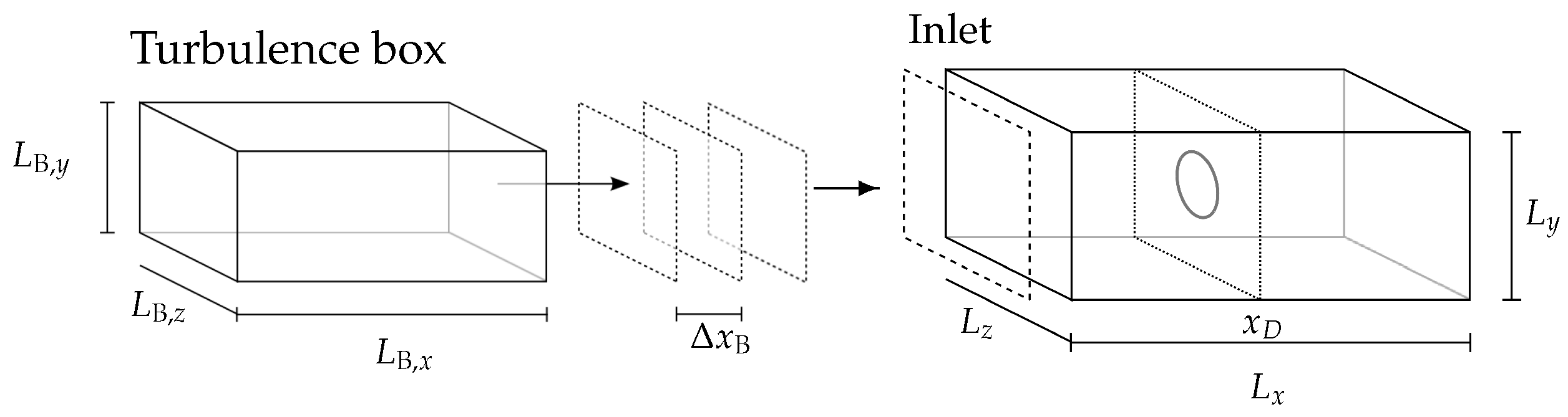
The first step of the investigation consists of the calibration of the parameters of the synthetic turbulence. This is finding ${\mathrm{TI}}_{\mathrm{B}}$ and $L_{1,\mathrm{B}}$ so that when a turbulence box is introduced in the computational domain, the desired target values are attained after a distance of $5D$, at $x_D$. The parameters of the synthetic turbulence for all boxes are shown in

Table 3. Characteristics of the different boxes of synthetic turbulence used as inflow for the LES.

	${\mathbf{TI}}_{\mathbf{B}}$ [%]	${\mathit{L}}_{1,\mathbf{B}}\times {10}^{-3}$ [m]	$\mathit{k}/\frac{1}{2}{\mathit{U}}_{\mathit{\infty }}^2$ [-]
Case Ti3	35.0	5.82	0.37
Case Ti12	60.2	15.3	1.08

. These were computed longitudinally and averaged over the whole volume. It is immediately noticed that high TI values were necessary to reproduce the evolution of the turbulence intensities reported by the experiments. Consequently, the approach followed could be seen as rather crude, on account of the Taylor approximation. However, the results reproduce, for the most part, the longitudinal evolution of turbulence predicted also by the empirical relations found in the literature. 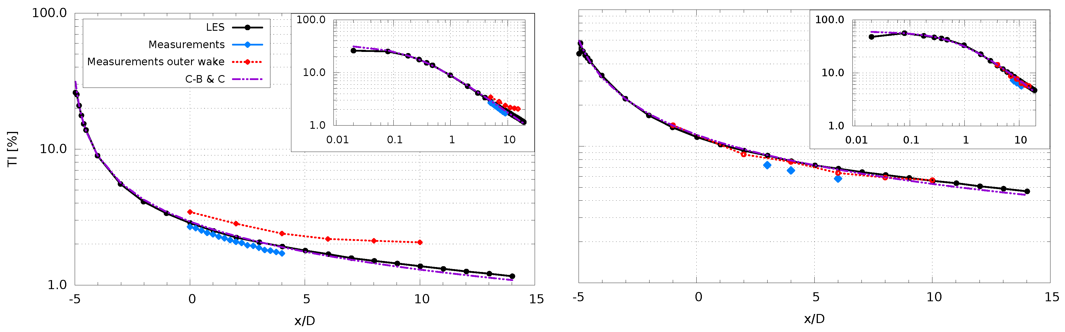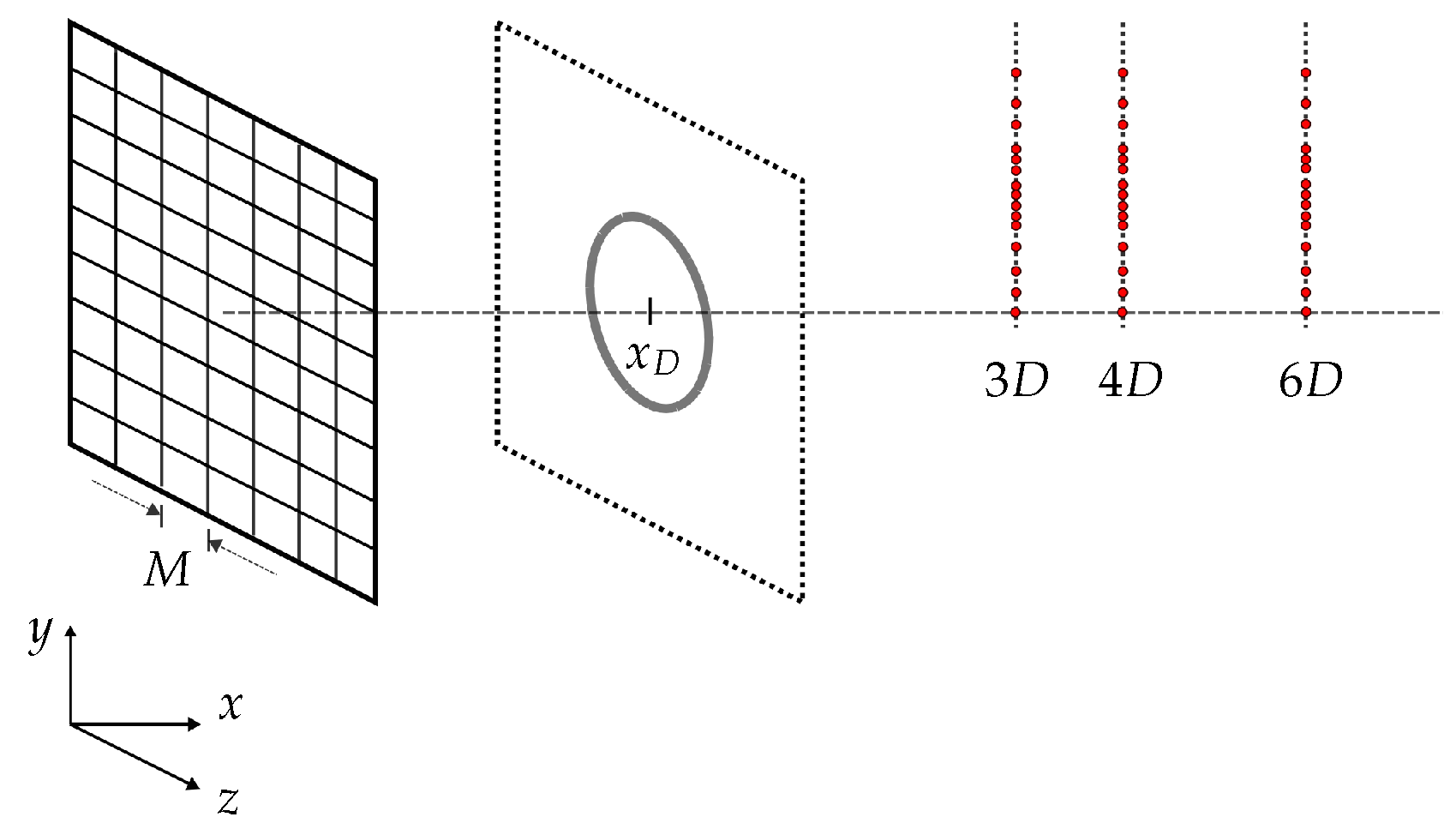This can be seen in Figure 3, which shows the free (no disk) homogeneous turbulence decay in each TI case obtained with LES. There, every value represents the average of the TIs computed from time-series stored in nine probes distributed in a crosswise plane, in turn located at every longitudinal position indicated by the marks in the curves. LES results are compared to the values measured in the wind tunnel and to the least-squares fit with Equation (4). As mentioned in Section 3, experimental values from [16] are used in the Ti3 case. To complement HWA data (which in the Ti12 case has only 3 points), LDA measurements are used, obtained in the experiment with the low thrust disks but outside the wake envelope ($y=\pm 1$D). It can be seen that for both Ti3 and Ti12 the decay predicted by the LES follows fairly well the experimental values. The subframes in Figure 3 represent the same data but plotted in a log-log scale, so the power law decay of the TI (of slope $-n$ in Equation (4) can be better appreciated. This permits seeing that, after some distance, the decay rate is approximately equal for both TIs. Furthermore, it is also seen that the LDA (measurements outer wake) in the Ti3 case deviates from a constant decay rate and therefore from the LES. Conversely, the LDA data in the Ti12 compares very well with the LES prediction.

Equation (4) is an empirical relation first proposed by [41] to describe the decay in homogeneous turbulence seen in a wind tunnel. The applicability of this relation has been proven in a wide range of Re flows in later work [39,42,50,51]. In most of the results reported in the literature, a fit is produced setting the virtual origin $x_0$ to zero in the equation, which neglects the agreement close to the grid or the place where turbulence originates as the stations where measurements or calculations are reported are generally far from such region. However, as the complete evolution of TI is monitored, a better fit is obtained by setting $x_0$ to a position different from where the turbulence is introduced (in particular, to an upstream location). The fit of Equation (4) for the curves shown in Figure 3 yields the results shown in

Table 4. Parameters of the fit of TI decay of LES to Equation (4). $x_0$ denotes the virtual origin of the curve with respect to the inlet.

	${\mathit{x}}_0=0$		${\mathit{x}}_0\ne 0$
	$\mathbf{1}/\mathit{A}$	$\mathit{n}$	$\mathbf{1}/\mathit{A}$	$\mathit{n}$	${\mathit{x}}_{\mathbf{0}}$ [m]
Case Ti3	24.11	1.281	9.85	1.519	−0.021
Case Ti12	28.49	1.15	11.43	1.661	−0.0845

. If the fit is made using $x_0=0$, the parameters are closer to those reported in the literature (see Section 2), although the curve would display a much higher TI at the inlet than the one given with $x_0\ne 0$, this is, ∼60% for Ti3 and ∼100% for Ti12. The mesh spacings used for the fits are $M=0.0225$ m for Ti3 and $M=0.20$ m for Ti12. The problem of setting $x_0$ has been discussed by [52], which show that when $x_0$ is properly determined, its value and the exponent of the power law decay n is Re-independent, while A is indeed a function of initial conditions (including Re), so the turbulence decay takes a universal self-similar behaviour.

Table 3 also shows the magnitude of the $L_{1,\mathrm{B}}$ in the synthetic turbulence. According to these results, it is seen that the requirement of two cells per $L_1$ (assuming the applicability of the minimum condition to represent a wavelength [53]) is sufficiently fulfilled. In effect, for the case Ti3, $L_1/\Delta \simeq 3$ is obtained. The resolution of eddies is somewhat improved in the case of Ti12, where $L_1/\Delta \simeq 4$. These resolutions that seem a priori rather coarse are the result of a series of compromises that have been previously explained. In [30] a similar resolution was used for the synthetic inflow in LES computations of the wake of a rectangular channel, obtaining a good comparison with experimental results related to the flow structures. The results of the turbulence decay in the absence of the disk show that these values are enough to supply an integral lengthscale to procure the desired magnitudes $L_1=0.01$ m (Ti3) and $L_1=0.03$ m (Ti12) at $x_D$. 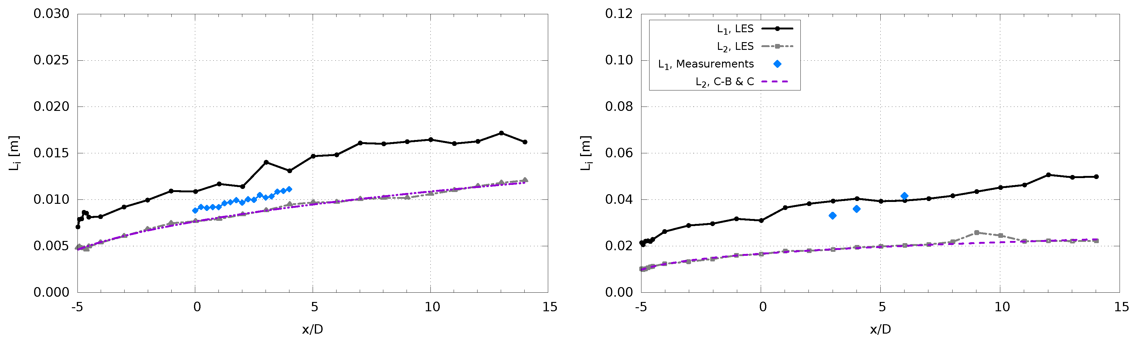Figure 4 shows the development of the longitudinal and transversal integral lengthscales, $L_1$ and $L_2$, along the flow. These are computed using velocity time-series (recorded at the same positions for TI above) and employing the method described in Section 4.4. The measurements from [16] are also used for comparison in the Ti3 case. There, the comparison of the measurements with the LES shows a small overestimation of $L_1$, although it should be considered that the difference is increased in the figure as the experimental value is below the target $L_1=0.01$ m. A fit of Equation (5) is also made for $L_2$ obtained with LES. In the Ti3 case, the least-squares fit method applied yields $B_1=0.089$, $n_1=0.392$ and an origin set at $x_0=-0.188$ m (upstream) from the inlet. Therefore, according to reference values provided along Equation (5), the LES slightly overestimates $L_2$ for Ti3. In the Ti12 case, the comparison with measurements is made with the only three points available so it is less decisive, although they suggest a higher growth rate. The fit of Equation (5) to the LES predicted $L_2$ yields $B_1=0.064$ and $n_1=0.254$ with $x_0=-0.068$ m, which, compared to the values in the literature, also indicates a slight overestimation by the computations. For the purposes of this work and considering the mesh restrictions, the development of the integral lengthscales in the flow predicted by the LES is deemed satisfactory.

In both TI and $L_i$ results, we can observe small oscillations for the first positions next to the inlet, which are likely the result of the adjustment of the synthetic velocity field to the LES. Specifically, the incompressibility conditions imposed by the solver as the original formulation of the Mann algorithm does not produce divergence free fields, as pointed out by [29].

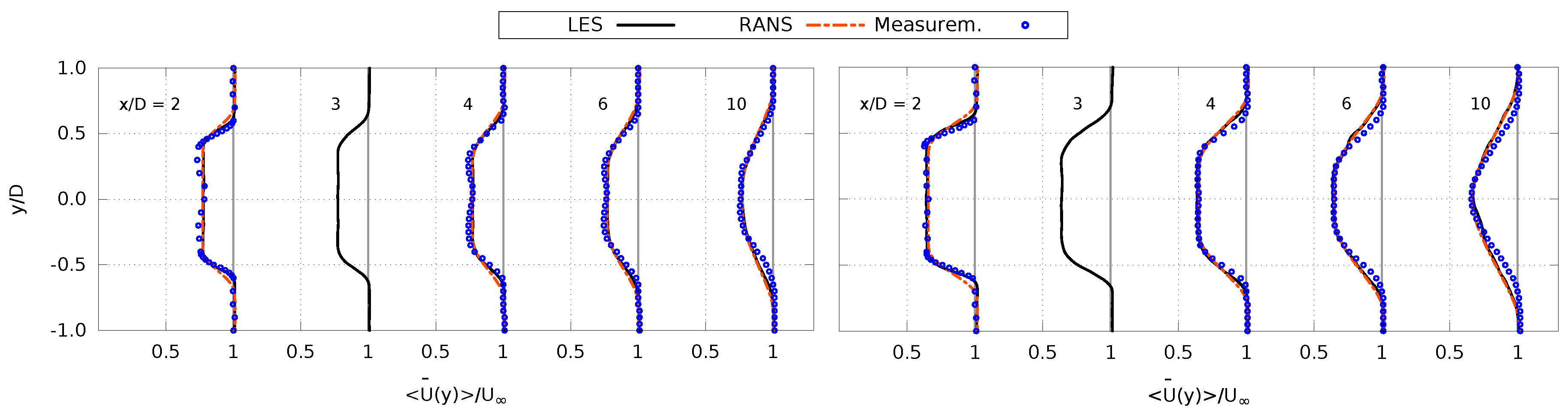
5.2. Velocity Deficit

The results for the wake simulations obtained with the AD are now shown. The first comparison is made from the results of the streamwise velocity deficit along the vertical direction at different longitudinal positions, normalized by the freestream velocity at $y=1.5D$. For these and other quantities extracted across the wake field shown in Section 5.2, Section 5.3, Section 5.4 and Section 5.5, the values are sampled at every cell centre along a line in the y-direction (at the mid-plane $z=0$) at different $x/D$ positions. These quantities correspond to time averages made during 20 LFT (13.33 s). No further spatial averaging is made. Note that LES results at $x=3D$ have been added to the available x-positions of the LDA data as this is a position where values computed from HWA are later shown.

Figure 5 shows the results for the high and low solidity disks under the inflow Ti3. The agreement to the experimental results is very good, with the larger difference observed around the shear layer (i.e., the wake envelope at $y\simeq \pm 0.5D$) from the disk edges, especially for the disk with higher thrust.

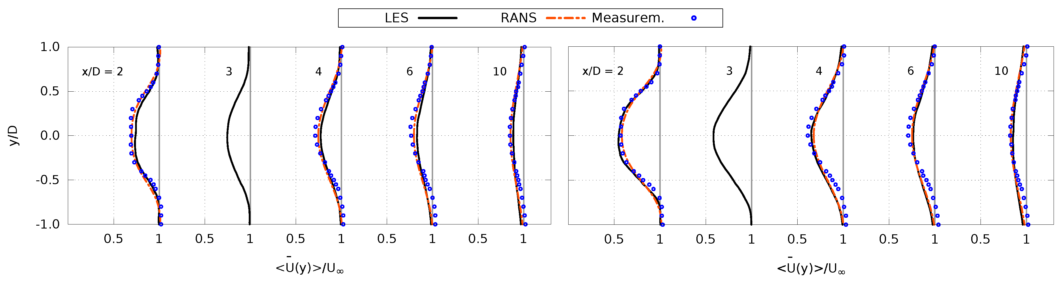
In the case of the Ti12 inflow, Figure 6 shows a minor reduction in the agreement of the LES with the measurements. The predictions commence to differ when moving further into the far wake, around the centreline and shear layer regions. Remarkably, the results of RANS are almost identical to those from LES in both TI cases.

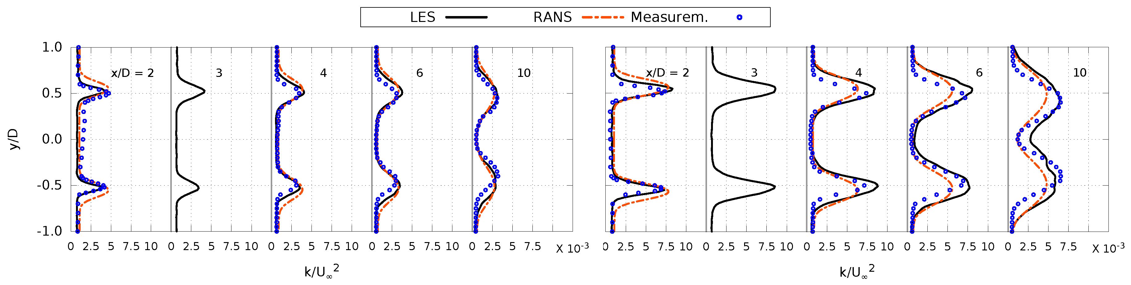
5.3. Turbulence Kinetic Energy in the Wake

It is expected that the wake created by the disks augments the turbulence level with respect to the ambient value. It is now investigated how the computations of the added turbulence compare to the experimental results within the wake. Figure 7 shows the profiles of k (this is, $k_{tot}=k_{\mathrm{SGS}}+k_{res}$ for the LES) at different downstream positions along the wake, when the inflow of the case Ti3 is used. There, it is observed that the LES results match quite well the measured (LDA data) turbulence levels behind both disks. However, it is noticed that, except for the nearest position to the disk, the LES predicts a higher diffusion of shear turbulence in the crosswise direction, an effect that is increased with the disk thrust.

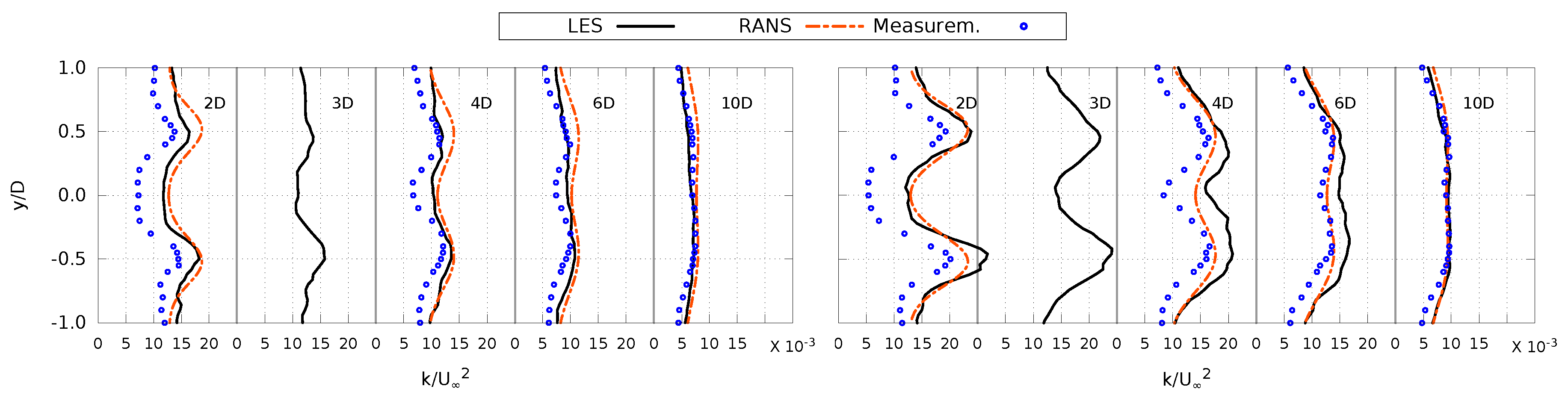
For the disks in the Ti12 case in Figure 8, the LES compare mostly well with the experimental data, although a small overestimation of k can be seen just behind the disk ($x=2D$). It is also observed that the shear layer originating at the edges of the disk is mixing faster with the ambient turbulence compared to the Ti3 inflow. Indeed, the effect of shear prevails deeper into the wake in the LES with the highest thrust disk, whereas it is mixed faster into the ambient turbulence when the thrust is lower. Results from the RANS computations are discussed in the next section.

It is also noticed that some inhomogeneities appear along the curves of LES, very noticeable in the simulations with the Ti12 inflow. These seem to indicate a footprint of the turbulence structures of the inflow turbulence. Although this feature could provide evidence of the need of performing averages in the azimuthal direction or creating synthetic turbulence that would cover longer simulation periods, it is thought that the results shown in the figures are sufficient for the purpose of these comparisons.

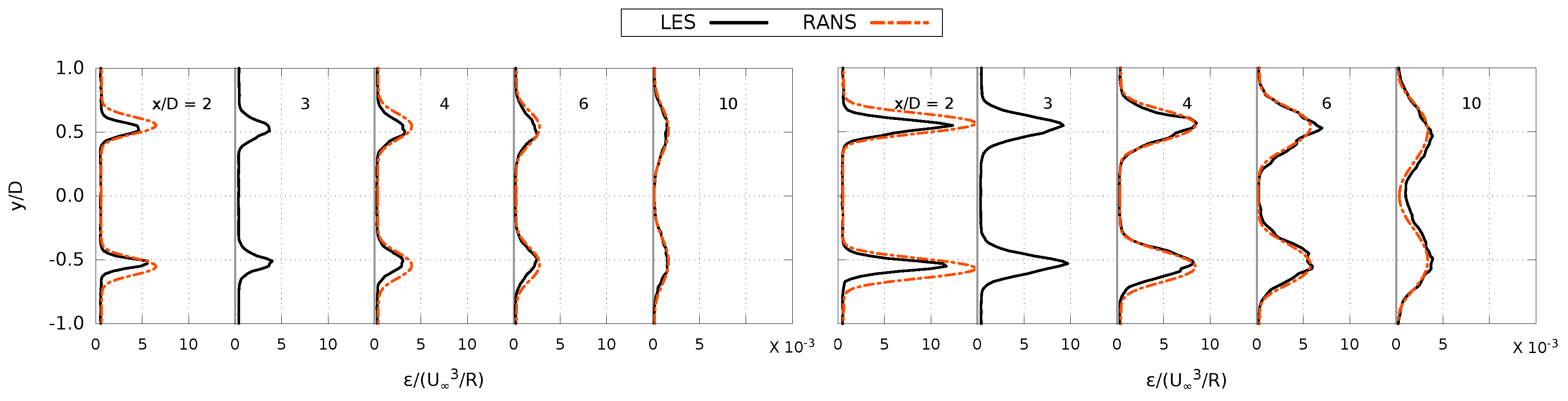
5.4. Turbulence Dissipation in the Wake

In the LES computations, the dissipation shown corresponds to ${\epsilon }_{tot}={\epsilon }_{res}+{\epsilon }_{\mathrm{SGS}}$. The dissipation is calculated from the HWA data using Equations (2) and (3), which was only available in the Ti12 case. Therefore, results of Ti3 are shown only for completeness in Figure 9, where it can be seen that, as before, differences between LES and RANS are small, as the curves differ only at $x=2D$ where RANS predicts a higher dissipation within the shear layer.

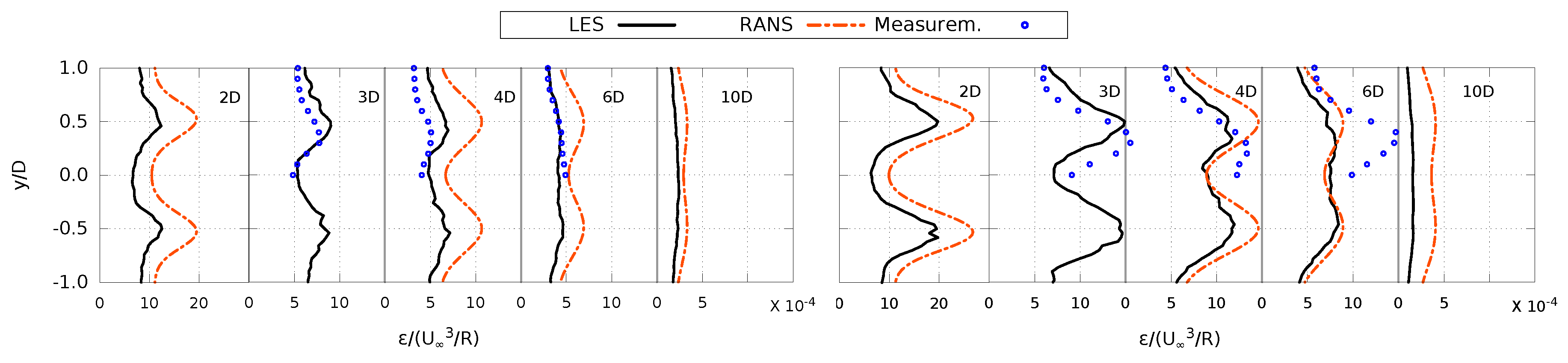
For the results with the Ti12 inflow in Figure 10, it is seen that, for the disk $C_T=0.45$, the LES predictions compare well with measured values. For the disk $C_T=0.71$, the measurements reveal a large increase of dissipation within the shear layer, compared to the data of computations with the lower thrust AD. Furthermore, at least within the three longitudinal positions available, measured dissipation in the shear layer is more or less maintained. The computations with $C_T=0.71$ also display a somewhat stronger mixing of turbulence from $x=4D$, where dissipation becomes more uniform and less predominant in the shear layer.

The RANS computations with the modified $k-\epsilon$ model of Sumner and Masson have been previously shown capable of reproducing the turbulence level in the wake [17]. In the present comparison, it is seen that for the Ti3 inflow the agreement is very good for the disk $C_T=0.42$ while it falls somewhat behind in the far wake of $C_T=0.62$. However, in both cases, the agreement in the computed dissipation of RANS and LES is very good except for $x=2D$. Interestingly, it is the vicinity of the disk where the k-$\epsilon$ is often corrected by adding dissipative terms to the $\epsilon$ equation to overcome the miscalculated turbulence stresses [49]. The results with the Ti12 show the opposite picture with regard to the estimation of k, as the agreement with measurements becomes better only for farther distances from the disk. For the closest position, the turbulence level is overestimated (as it is in the LES) despite the drop of the turbulence production terms near the disk ($x=2D$ is outside this region). Dissipation seems overestimated in the case of $C_T=0.45$ when comparing to the measurements. This is less certain for the higher thrust disk, where at $x=4D$ the peak value of dissipation seems equal to the measured one, but much smaller in the case of $x=6D$. Notably, $\epsilon$ from RANS is always higher than any LES in the wakes of the Ti12 inflow. Previous work [49] has shown that, in the ABL, the k-$\epsilon$ model overestimates the dissipation around the disk when comparing with LES. This has been observed to occur even upstream of the disk, where $\epsilon$ has been seen to increase unlike computations of LES, where this value does not grow until $0.5D$ downstream from the rotor.

It should be remarked that Sumner and Masson [17] showed that results with various turbulence closures (standard k-$\epsilon$, RNG, El Kasmi and Masson model [48] and their own model) compare, in essence, equally well to the measurements, with no apparent advantage of their proposed correction to the k-$\epsilon$ model (although $\epsilon$ yielded by the different closures was not compared). The fact that all models compare well to measurements appears to contradict the otherwise inadequate results obtained in simulations of wakes in the ABL flow cited in that work. There, it is also argued that this is due to the relative decrease of the modelled turbulent viscosity ${\nu }_t$ in the reproduction of wind-tunnel wakes with homogeneous inflow with respect to its proportion in the modelling of atmospheric flow. In those conditions, previous work by [49] has successfully proved the advantages of LES to estimate the velocity deficit and turbulence levels in the wake.

5.5. LES Modelling in the Wake

The previous results for k and $\epsilon$ indicate that the LES running in OpenFOAM is able to predict with relative accuracy not only the velocity deficit in the wake, but also the level of turbulence and its dissipation in the case where the TI in the inflow is low (∼3%). For the high TI inflow (∼12%), the prediction becomes more imprecise, according to the comparison with the experimental data. In the absence of disks, it is observed that the fraction of the turbulence kinetic energy that is resolved by the LES with respect to the total $k_{res}/k_{tot}$ occurs for the most part in the resolved scales, at around 90% in both TI cases throughout the domain and only somewhat smaller close to the inlet [54]. With the introduction of the disks, this does not appreciably change except for the shear layer nearby the AD at around $x=1D$ in the Ti3 case, where the resolved part is slightly reduced [54]. In the Ti12 case, this difference is not noticeable and the value of $k_{res}/k_{tot}$ remains throughout.

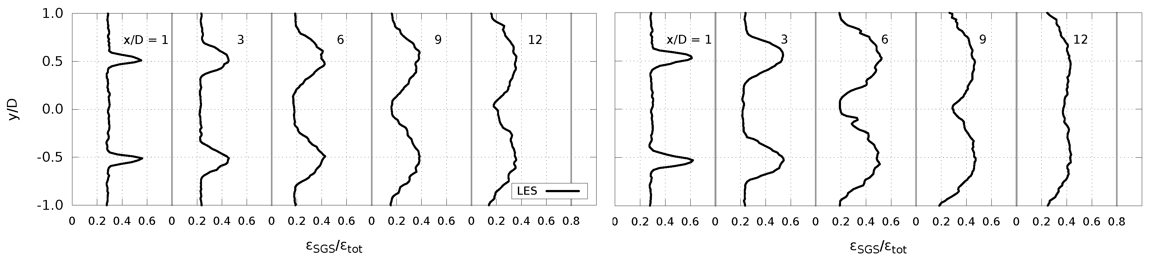
Figure 11 shows the ratio of subgrid dissipation with respect to the total value ${\epsilon }_{\mathrm{SGS}}/{\epsilon }_{tot}$ along the wake for the Ti3 case. Note that, as the positions of comparison are no longer restricted to those of the available experimental data, profiles are shown at different longitudinal positions from other figures. In Figure 11, it is noticed that the LES has an appreciable increment in subgrid dissipation within the shear layer. Furthermore, this increase persists longitudinally even as far as when the wake appears to reach a state of transversally-uniform dissipation, i.e. at $x=12D$ with disk $C_T=0.62$. This is consistent with the hypothesis that turbulence is created at smaller lengthscales than the ambient turbulence at the disk edge. Due to the limited resolution of turbulence lengthscales in the Ti3 flow (missing in the synthetic flow as well), the increase in subgrid dissipation is produced at scales that seem absent in the incoming flow. These results also show that the wake envelope becomes the main carrier of dissipation. The subgrid dissipation part is also larger with higher thrust, yet by a small margin. 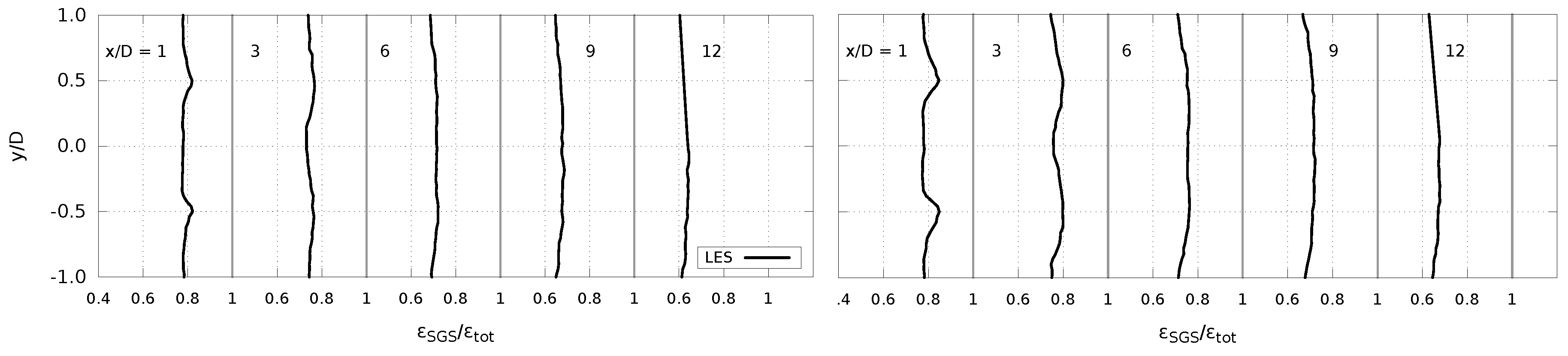It is observed that, in the absence of disks, most of the dissipation comes from the resolved fluctuations, in a proportion very similar to that shown outside the wake, at $y\pm 1.0D$ [54]. It is seen in Figure 12 that when the inflow turbulence raises (which comprises better resolved lengthscales), the increment of subgrid dissipation in the region of the wake envelope is greatly reduced. As a result, the modelling ratio seen outside the wake is essentially conserved. From these results, it can be deduced that the LES modelling across the wake is largely determined by the ambient turbulence.

5.6. Integral Lengthscale in the Wake

The changes in $L_1$ caused by the presence of the AD and the wake are now investigated. The computation of $L_1$ is performed as described in Section 4.4, which involves the assumption of the Taylor hypothesis to transform the computed time-scales into lengthscales. Evidently, this supposition becomes more difficult to accept when shear is present in the flow. However, previous work has reported satisfactory results in wake studies that support the continuing applicability of the hypothesis. For instance, Ref. [16] has compared the lateral distribution of $L_1$ behind the wake produced by a porous disk (in a setting similar to the experiments used in this work) computed from HWA with the one obtained from PIV. They did not find a difference in the results obtained from either technique, despite the fact that HWA uses the local mean velocity to calculate the lengthscale, compared to the direct spatial measurement offered by PIV. Making the same assumption, the evolution of the integral lengthscale behind the AD computations is studied.

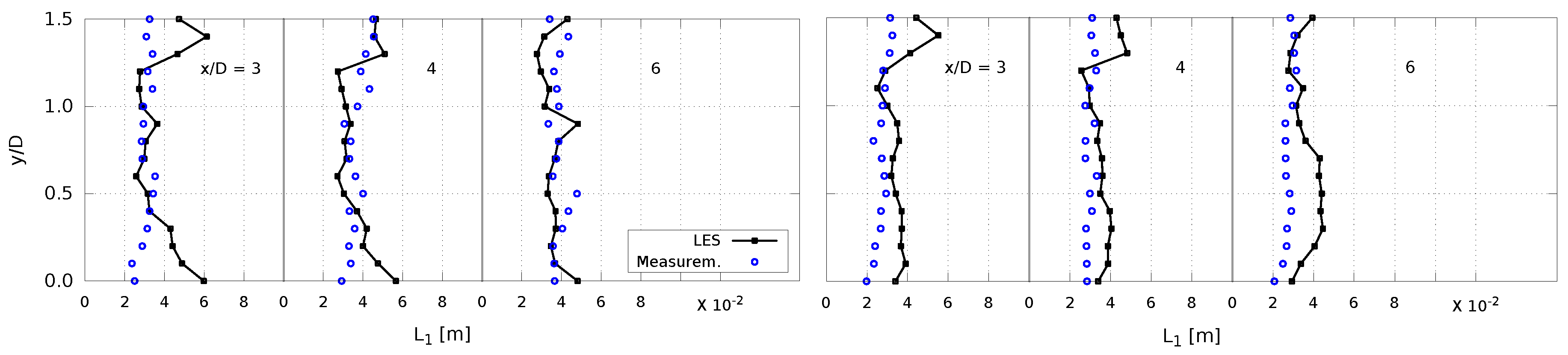
Figure 13 displays the values of $L_1$ computed from the LES in each code with the Ti3 inflow, from $y=0$ to $y=1.5$, at $3D$, $4D$ and $6D$, which correspond to the positions where HWA data for the Ti12 inflow is available. It is first noticed that there is not a clear influence of the shear layer in the size of the turbulence scales. However, for a region about $0.5\le y/D\le 1.0$, next to the the shear layer, larger lengthscales can be discerned amongst the variations in the profile. Indeed, the maximum values of $L_1$ at each $x-$position are at close $y=0.5D$ in the wake of the disk $C_T=0.42$. This is consistent with the previous results with regard to the location of the shear layer along the wake (e.g. k and $\epsilon$). Conversely, for the other disk the maxima of $L_1$ would suggest a wake that expands to about $y=0.75D$ at $x=6D$, which is larger than what the previous computations indicate.

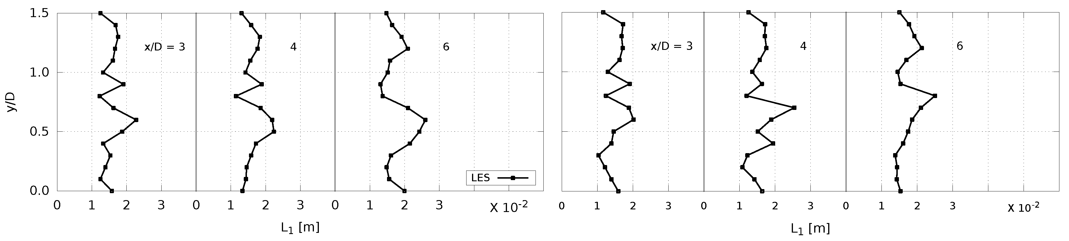
Results for the Ti12 inflow are shown in Figure 14. Notably, the computed values from the experimental time-series do not reveal a variation of the lengthscale values at the shear layer. In fact, there is no evident change in $L_1$ within the wake. This trait is similarly observed in the LES results. The only variations in computations are observed at the upper part of the curves or, in the case of the disk $C_T=0.45$, towards the bottom part where $L_1$ is larger (but this effect is reduced further downstream).

Previous experimental work by [16] showed that in the wake of a porous disk with a solidity of $45\%$, $L_1$ is approximately 1.5 times larger within the shear layer with respect to the values within the wake or outside the envelope. However, these measurements were obtained using an inflow with very low turbulence ($\mathrm{TI}<0.4\%$), which clearly sets a different scenario in comparison to this study. Precisely, the absence of a variation of $L_1$ in the shear layer can be explained considering the previous results, which point at a dominance of the ambient turbulence characteristics over the wake in the case of the inflow Ti12. Although the turbulence production is visibly higher when the disk thrust is larger (Figure 8), its effect does not appear to have an impact on the turbulence lengthscales. Similarly, the use of a lower turbulence inflow (Ti3) does not seem to decidedly increase the magnitude of the lengthscales in the area of turbulence production, or at least not in the computations performed for this work. In this regard, the fact that the characteristic lengthscales of the Ti12 inflow are better resolved by the mesh and the LES compared to the Ti3 cases can be a factor to consider. This is, if resolution is not adequate within the shear layer, it is to be expected that a sizeable part of the turbulence being produced would fall into the modelled part instead of being resolved, therefore affecting the magnitude of the computed scales. This has been studied in Section 5.5, where it is shown that the LES modelling does not vary within the wake with respect to the external flow aside from very close to the disk ($x=1D$) in both codes. Nevertheless, it has been seen that despite the limited resolution, the LES computations have been able to reproduce other principal features along the wake, such as the turbulence levels.

5.7. Spectra behind Disks

To study the redistribution of turbulence energy along the wake, the spectra obtained at different longitudinal positions for every disk are compared with the spectrum of the free decaying turbulence. Power Spectral Density (PSD) curves are calculated from only one measuring position at centreline, so to reduce the noise in the spectral curves, the time-series of each register are divided into eight non-overlapping blocks with an equal number of samples. Then, the PSD of all blocks are averaged to produce the curve at each longitudinal position. However, noise remains along the curves that make the comparison very difficult, so a smoothing procedure is needed to be performed. To this aim, an exponential moving average is used to filter the spectra computed at each longitudinal position (a rational transfer function is employed, see [55]). Hence, the spectra shown in the following figures have been processed with this technique, with the sole exception of that obtained from measurements without a disk, which was spatially averaged with results obtained at the other eight locations distributed crosswisely. As the spectra are calculated from data at a fixed location (sampled in time), the Taylor hypothesis is applied to transform the frequency spectra into a wavenumber spectra using ${\kappa }_1=2\pi f/〈U〉$, where f is $f_{acq}$ for measurements or $f=1/\Delta t$ for the LES. In this way, it is possible to also compare with the PSD from the synthetic turbulence, which is calculated as the volume average of the spectra computed in the longitudinal direction.

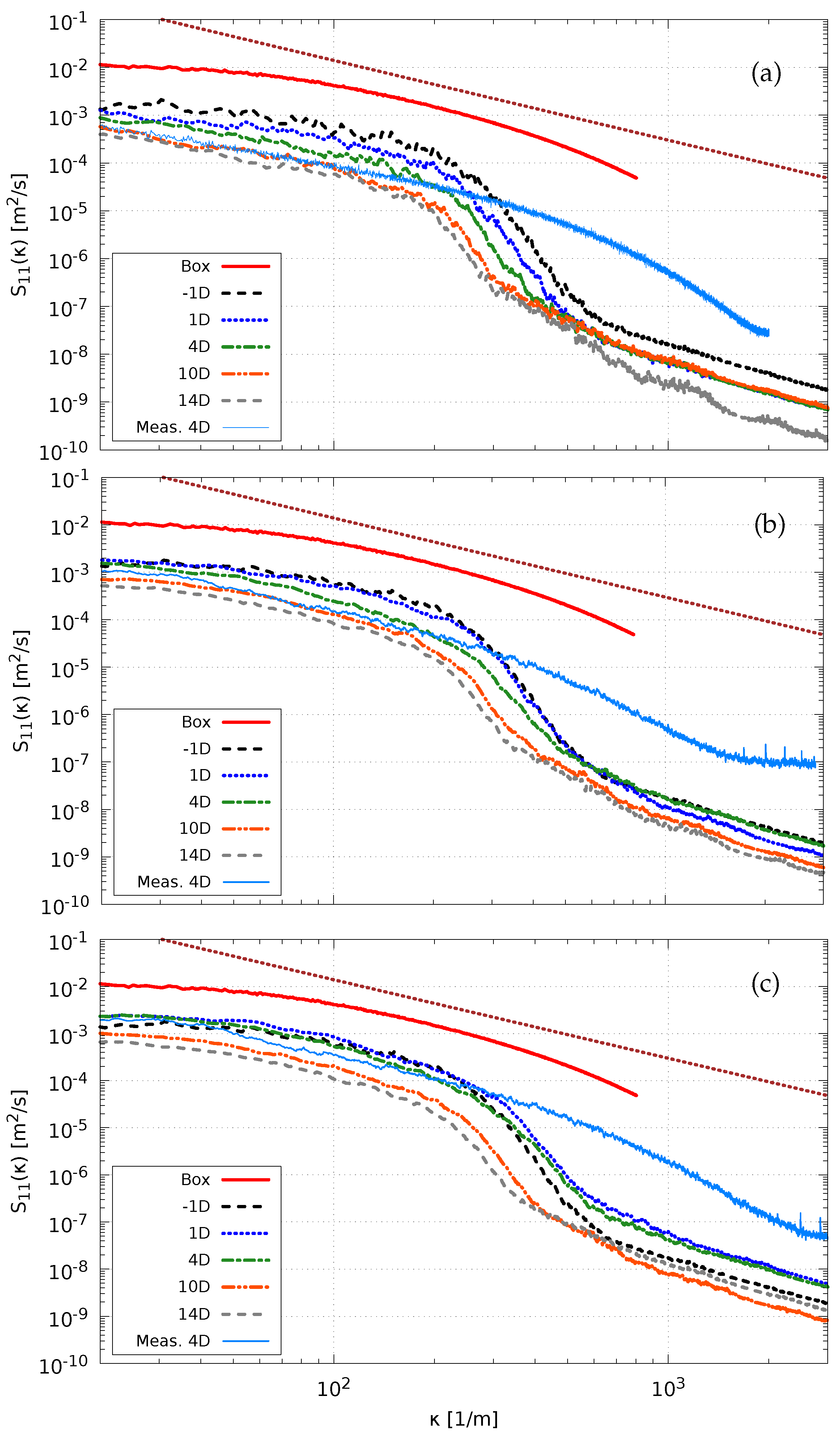
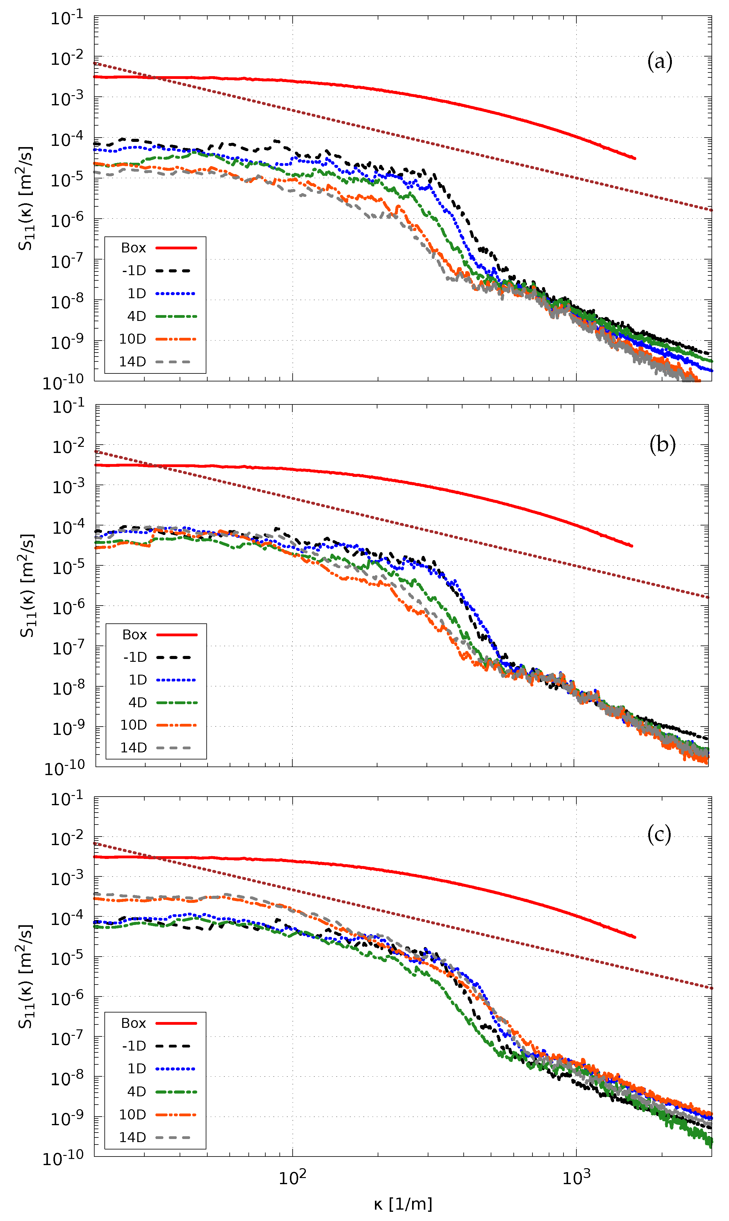
The results for the inflow Ti3 are shown in Figure 15. In the results without the AD, a constant decay of energy is observed as the flow moves downstream. The spectra from the synthetic box serve to mark the extension of the resolved wavenumbers (${\kappa }_{max}=\pi /\Delta =1571$ m⁻¹) since the spatial resolution in the box is the same as in the LES. Note that the abrupt drop in the turbulence energy spectra is attributed to a combination of numerical diffusion and the limited spatial resolution [5]. In case of the disk $C_T=0.42$, a gain in turbulence energy is seen immediately behind the disk, as the curves at $-1D$ and $1D$ are almost identical. A small decay of energy is observed at $4D$ and, from there, an increase in turbulence energy around the highest levels (lowest $\kappa$). For the disk $C_T=0.62$, the effects are accentuated, and the curves at $4D$ are the only ones displaying a decay and yet only around the inertial range. The energy of the next two longitudinal positions, $10D$ and $14D$, increases for all wavenumbers, which represents an increment of about one order of magnitude at the lowest wavenumber, with respect to the levels displayed by the decaying turbulence without disks. Notably, the spectra of the last two positions seemingly exhibit an inertial range, characterized by the slope of $-5/3$ in the decay rate.

The results for the Ti12 inflow are shown in Figure 16. In this case, the spectra computed from experimental results are also included. The spectra obtained from measurements with disks extend to larger wavenumbers than in the cases without disk, due to the use of a different frequency in the low-pass filter. For the case without disks, the energy at the lowest wavenumbers obtained from the LES proves to decay less as it has been shown before. However, they display a steady decay that adjusts well to the characteristic slope of the intertial range, also discernable in the experimental results. These observations are analogous for the results with the disk $C_T=0.45$. In contrast to the Ti3 inflow where energy is seen to increase beyond $x=4D$ for the disk with the same porosity, here a reduction in the contribution of shear towards the increase of energy along the wake is observed. Although the overall levels of turbulence energy in the wake are higher than in the free decaying turbulence, they maintain more or less the same relative decay from one to another. This behaviour is similar in the case of the disk $C_T=0.71$. There, only the curve at $4D$ shows an increase in energy compared to the previous disk (also matching fairly well the experimental results in the inertial range).

5.8. Vorticity Contours

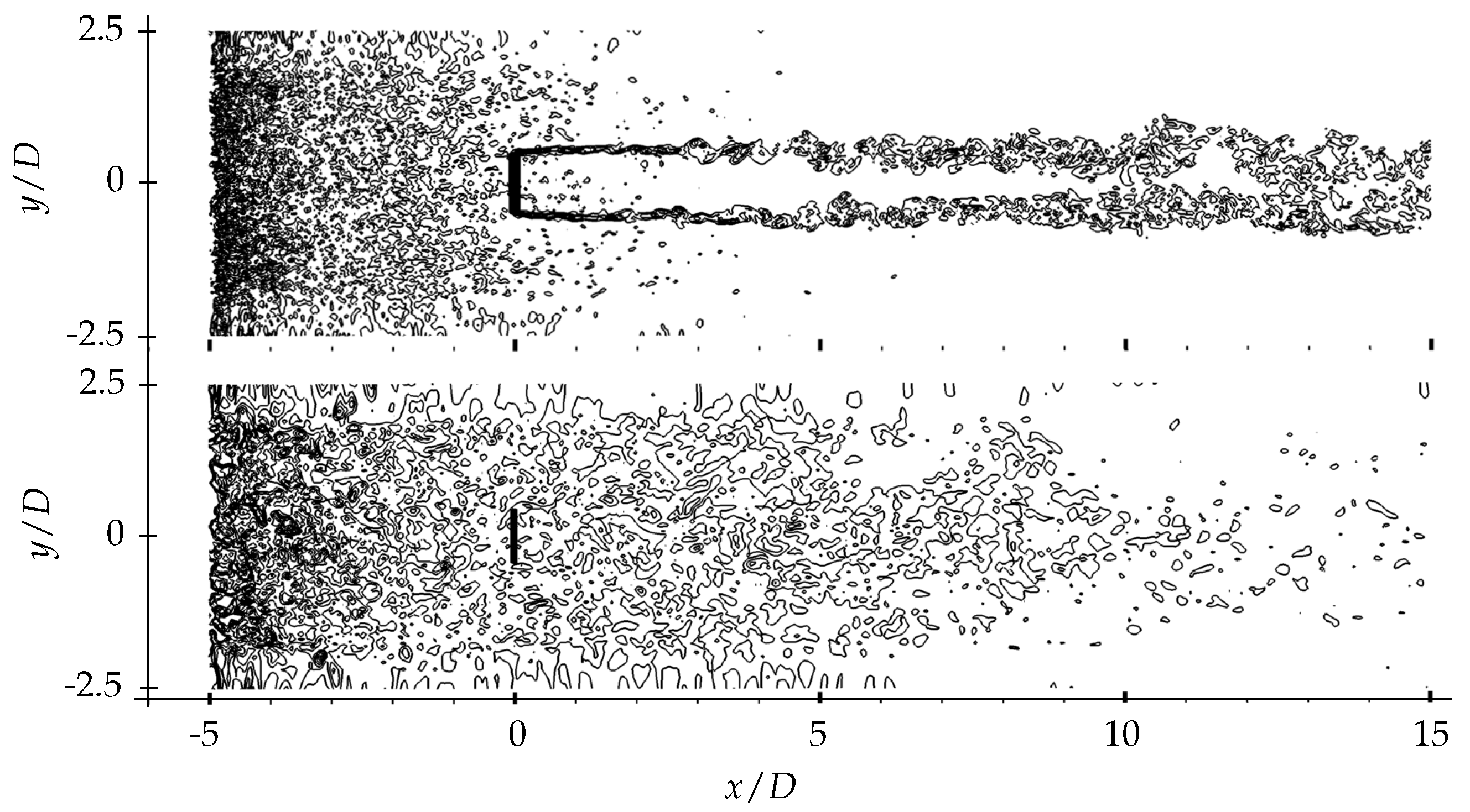
Lastly, to complement all previous results, Figure 17 shows a comparison between the the contours of vorticity obtained in the Ti3 and Ti12 cases and using the highest porosity disk, $C_T=0.62$ and $C_T=0.71$, respectively. The images are taken at the x–y plane, at $z=0$ and correspond to the vorticity field computed at the last time step of the LES runs. Make note that black bars are used to represent the disk position but do not portray the complete longitudinal region where the forces modelling the AD act, distributed using Equation (7). This figure permits visualizing the dominant effect of the turbulence structures from the inflow of the Ti12 case, which, unlike the Ti3 inflow, prevail along the wake. With the Ti3 inflow, there is a clear shear region arising from the edges of the disk with distinct turbulence structures. Conversely, with the use of the Ti12 inflow, the shear region is substantially less noticeable in the higher ambient turbulence. Indeed, the vorticity contours from the inflow appear to dominate in the vicinity of the AD. This is consistent with the comparison of k in Figure 5 and Figure 6, where its increase within the shear layer is less prominent with the increase of ambient TI. In Figure 17, it can also be seen that, for the Ti12 inflow, structures that appear to arise from within the wake become more apparent than those outside from approximately $x\simeq 6D$.

6. Summary and Conclusions

This work has been dedicated to study the flow characteristics as well as the modelling of turbulence in wakes produced by a porous disk. For this, disks of two porosities have been used as well as two instances of decaying and homogeneous turbulence inflows, identified by streamwise turbulence intensities (TI) of approximately $3\%$ and $12\%$ and corresponding longitudinal integral lengthscales ($L_1$) of $0.01$ m and $0.03$ m. To perform this study, a methodology has been developed and implemented in OpenFOAM that uses Large-Eddy Simulations (LES) to reproduce the main turbulence features of a turbulent flow generated in a wind tunnel. The Actuator Disk (AD) technique was used to model the porous disk and replicate the turbulence properties measured in the wake flow. The employed methodology is based on a procedure previously shown to provide good results in the simulation of wind turbine wakes in homogeneous turbulence and atmospheric flows. A comparison with prior work made with RANS was made wherever possible.

To reproduce the grid-generated turbulence in the wind tunnel, a synthetic field of homogeneous isotropic turbulence was introduced at the inlet of an LES. An analysis of the decaying turbulence simulated by the LES demonstrated that the simulations reproduce the TI decay and the evolution of $L_1$ predicted by the parametrizations predominant in the literature, in addition to replicating fairly well the experimental values at the measured locations. The wake field results obtained with the introduction of the AD showed a good agreement with the wind tunnel experiments for the velocity deficit, turbulence kinetic energy k and its dissipation $\epsilon$. It was also found that $L_1$ evolves, for the most part, as in the decaying homogeneous turbulence. Remarkably, there was no apparent variation of $L_1$ within the shear layer compared to the center of the wake or outside the wake envelope.

A study of how the LES performs in the wake was also carried out, with the main interest of observing how the modelling ratio (the contribution of the resolved or SGS parts to the total value) is affected by the regions of high shear behind the AD in comparison with the outflow and the center of the wake. It was found that while the modelling ratio of k in the wake is largely maintained with respect to the outside flow, the subgrid part of $\epsilon$ increases within the shear layer, but only when the low TI inflow is used. From the results, it is seen that modelling in the freestream flow prevails in the wake just as the level of inflow turbulence increases. On the other hand, the wake results compare well with the velocity and k obtained with RANS. Likewise, LES and RANS results of $\epsilon$ match also in the low TI case, whereas the values yielded by RANS seem overestimated—in comparison with both measurements and LES—in the high TI case, particularly in regions of strong shear.

Spectra computed at different axial positions in the wake reveal that shear causes a noticeable boost in the energy content of turbulence, but only in the low TI case. This causes that for the two furthermost positions ($x=10D$ and $14D$), the energy levels are higher or at least as energetic as in the upstream region near the disks. Moreover, the turbulence at those positions shows a clear inertial range that was absent in the decaying turbulence at low TI. Conversely, for the high TI inflow, it is seen that, despite the fact that turbulence energy levels rise in the wake with respect to the decaying homogeneous flow, the relative decay is maintained from one position to the other.

Considering the above, the central conclusions of this investigation are:

• The evolution of $L_1$ was not noticeably different in the wake in comparison to what was observed in the decaying homogeneous turbulence.
• Turbulence scales in the wake appear to be dominated by the inflow characteristics and this effect increases with the level of TI in the inflow.
• It is seen that the resolved/subgrid modelling ratio in the freestream flow prevails in the wake in relation to the increasing level of ambient turbulence.

The comparison of the LES with experimental results has permitted validating the methodology presented in this work as a suitable approach to investigate the turbulence features in the wake flow of wind turbine models. With this method, it can be possible to study the spatial and transient development of wake characteristics and assess the influence of, for example, a variety of inflow turbulence conditions or wind turbine models of varying sophistication. These aspects are considered for future work. In the same manner, an analogous study can be performed for an array of wind turbine models with the additional interest of observing the influence of downstream turbines in the wake turbulence field, for different layouts. Clearly, a CFD tool like the one presented in this work bears the advantage of changing the simulation setup without needing to perform new experiments each time, while also removing the spatial or temporal limitations associated with the measuring techniques.