Dynamic Denoising and Gappy Data Reconstruction Based on Dynamic Mode Decomposition and Discrete Cosine Transform

Abstract

Dynamic Mode Decomposition (DMD) is a data-driven method to analyze the dynamics, first applied to fluid dynamics. It extracts modes and their corresponding eigenvalues, where the modes are spatial fields that identify coherent structures in the flow and the eigenvalues describe the temporal growth/decay rates and oscillation frequencies for each mode. The recently introduced compressed sensing DMD (csDMD) reduces computation times and also has the ability to deal with sub-sampled datasets. In this paper, we present a similar technique based on discrete cosine transform to reconstruct the fully-sampled dataset (as opposed to DMD modes as in csDMD) from sub-sampled noisy and gappy data using $l_1$ minimization. The proposed method was benchmarked against csDMD in terms of denoising and gap-filling using three datasets. The first was the 2-D time-resolved plot of a double gyre oscillator which has about nine oscillatory modes. The second dataset was derived from a Duffing oscillator. This dataset has several modes associated with complex eigenvalues which makes them oscillatory. The third dataset was taken from the 2-D simulation of a wake behind a cylinder at Re = 100 and was used for investigating the effect of changing various parameters on reconstruction error. The Duffing and 2-D wake datasets were tested in presence of noise and rectangular gaps. While the performance for the double-gyre dataset is comparable to csDMD, the proposed method performs substantially better (lower reconstruction error) for the dataset derived from the Duffing equation and also, the 2-D wake dataset according to the defined reconstruction error metrics.

1. Introduction

Dynamic Mode Decomposition (DMD) is a concept that was first introduced by Schmid and Sesterhenn to study the spatial dynamic modes of fluid flow [1,2]. DMD approximates the nonlinear dynamics underlying a given time-varying dataset in terms of a linear auto-regressive model by extracting a set of mode shapes and their corresponding eigenvalues, where the mode shapes represent the spatial spread of dominant features and the eigenvalue associated with each mode shape specifies how that feature evolves over time in terms of the frequency of oscillation and the rate of growth or decay. Rowley et al. envisioned DMD as an approximation to the modes of Koopman operator, which is an infinite-dimensional linear representation of nonlinear finite-dimensional dynamics [3,4]. Even though DMD was initially meant to be used for extracting dynamic information from flow fields [2], soon it found new applications in other areas of study as a powerful tool for analyzing the dynamics of nonlinear systems. Kutz et al. [5] expanded the theory of DMD to handle mapping between paired datasets. Jovanovic et al. proposed the sparsity-promoting DMD (spDMD) to obtain a sparse representation of the system dynamics by limiting the number of dynamic modes through an $l_1$-regularization approach [6]. In 2015, the extended DMD (EDMD) was introduced by Williams et al. to approximate the leading eigenvalues, eigenfunctions, and modes of the Koopman operator [7]. The EDMD is a computationally intensive algorithm since it requires the choice of a rich dictionary of basis functions to produce an approximation of the Koopman eigenfunctions. The richer the dictionary is, the more time it takes to compute the inner products which are a key part of EDMD algorithm. In an attempt to overcome this issue, Williams et al. proposed the kernel-based DMD (KDMD) in 2015 [8]. In this approach, rather than choosing the dictionary of the basis functions explicitly, they are defined implicitly by the choice of a kernel function. The kernel function resolves the computational intensity issue of EDMD by finding the inner products of the basis functions without the need to having them defined explicitly.

An initial attempt for incorporating compressed sensing in DMD was made by Guéniat et al. [9], where a subset of an originally-large dataset was taken by non-uniform sampling and was used for finding the temporal coefficients (eigenvalues) through solving an optimization problem. Further, the corresponding modes were found by solving a set of linear equations which involved the fully-sampled dataset. This makes the proposed algorithm (known as NU-DMD) impractical in the case the fully-sampled dataset is not available. Another approach for incorporating compressed sensing in DMD (known as csDMD) was developed by Kutz et al. [10]. In csDMD, the DMD eigenvalues are obtained from a sub-sampled dataset (similar to NU-DMD), which has the advantage of reducing computation time, and then the full DMD mode shapes are reconstructed through using an $l_1$-minimization scheme based on a chosen set of basis vectors. In contrast to NU-DMD, csDMD does not need the fully-sampled dataset in order to recover the mode shapes.

One of the initial attempts to deal with the issues involved in recovering a dataset from gappy data is presented in [11]. The proposed method relies on the presence of a set of empirical eigenfunctions, which represent an ensemble of similar datasets, and hence, the fully-sampled dataset is reconstructed based on these empirical eigenfunctions. In the case there is no such set available, they described a technique to build one from an ensemble of marred samples. In the case of marred samples, it is assumed there are several marred samples taken from each face, each one taken with a different mask. In addition, it is implicitly assumed that for each pixel there is at least one sample available. If there is a pixel which is not included in any marred sample, this method cannot recover it. Another well-known method for gappy data reconstruction is the Gappy Proper Orthogonal Decomposition (POD) method [12,13], which was proposed as an extension to POD considering the incomplete datasets. POD captures most of the phenomena in a large amount of a high-dimensional dataset while representing it in a low-dimensional space which causes a significant reduction in required computational power [14]. This technique has been used in various problems such as fluid dynamics [14], active control [15], and image reconstruction [16,17], to name a few. The original POD uses the fully-sampled dataset in order to reconstruct the POD basis functions. Even though Gappy POD aims at reconstructing gappy datasets, it, in fact, relies on the presence of a set of completely-known standard POD basis vectors which we believe makes the whole method inapplicable when there is no such set available. Also, a POD-based method for denoising and spatial resolution enhancement of 4D Flow MRI datasets is proposed by Fathi et al. [18]. This method uses a set of POD basis vectors as the reconstruction basis where the set of POD basis vectors is derived from the results of a computational fluid dynamics (CFD) simulation. Even though this method was shown to outperform the competing state-of-the-art denoising methods, the fact that it is specifically developed for noisy 4D Flow MRI datasets makes it impractical for the datasets resulting from other types of dynamic systems. None of these methods take into consideration the dynamics of a given dataset.

In the work presented here, an approach similar to csDMD was taken. With csDMD, the aim is to reconstruct the DMD mode shapes based on some given set of basis vectors, whereas, in our approach, called DMDct hereafter, given the DMD eigenvalues obtained from the sub-sampled dataset, the full dataset is reconstructed through an $l_1$-minimization scheme. Similar to csDMD, DMDct relies on the proper choice of the underlying basis functions. In this paper, we specifically focus on 2-D problems defined over a rectangular grid of equally-spaced nodes. By considering this specific geometry, we can take the one-dimensional discrete cosine transform (DCT) basis vectors and use them for building the two-dimensional basis vectors implicitly, hence requiring less memory.

2. Method

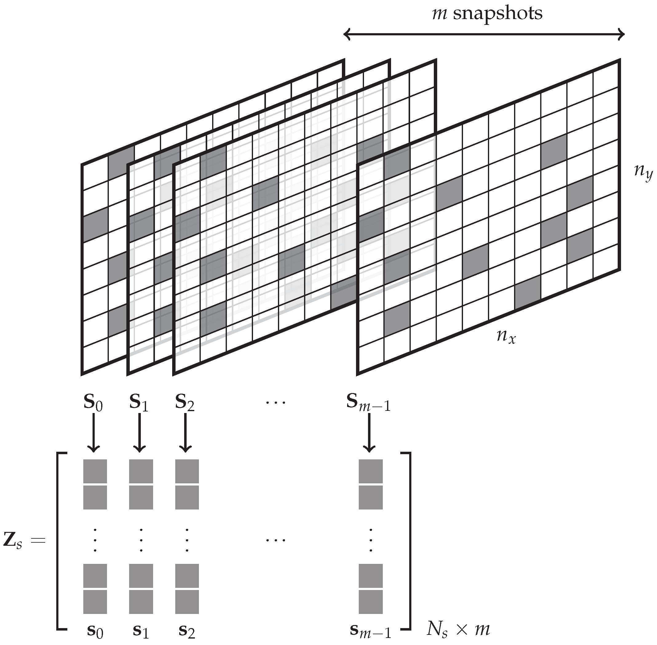
The DMDct method is derived for real-valued two-dimensional problems defined over a rectangular mesh of equally-spaced nodes as depicted in Figure 1. For each snapshot, only a subset of its elements is observed which is obtained by applying a pre-defined random sampling mask. The mask is defined as a set of pairs of $(i,i^{\prime })$ indices, shown as M, for which the samples are taken. All observed elements of each snapshot ${\mathbf{S}}_k$ are vectorized and represented as a real-valued data vector ${\mathbf{s}}_k$ of length $N_s$, where $N_s$ is the number of sampling points. The data vectors ${\mathbf{s}}_k$ are taken as the input to the DMDct algorithm. First, the $N_s\times m$ matrix ${\mathbf{Z}}_s=\left[{\mathbf{s}}_0\dots {\mathbf{s}}_{m-1}\right]$ is constructed and the exact DMD method is applied to that to obtain DMD eigenvalues $\mathbf{\lambda }$ (Section 2.1). Then, the spatial component of DMD is reconstructed based on the DCT basis vectors by taking random samples from the fully-sampled dataset while maintaining the sparsity of reconstruction coefficient matrices through an $l_1$-regularization scheme (Section 2.2). Finally, each snapshot is reconstructed in full using the calculated reconstruction coefficient matrices and the DCT basis vectors.

2.1. Exact DMD

The Exact DMD method [5] is briefly introduced here since DMDct relies on that for finding the eigenvalues and reconstructing the data. Given a sequential set of m data vectors ${\mathbf{z}}_k$ shown as an $N\times m$ matrix $\mathbf{Z}=\left[{\mathbf{z}}_0\dots {\mathbf{z}}_{m-1}\right]$, the exact DMD method gives us the set of r DMD modes ${\mathbf{\varphi }}_j$ and their corresponding eigenvalues ${\lambda }_j$ (Algorithm 1). The DMD modes and eigenvalues together describe how each vector ${\mathbf{z}}_{k-1}$ evolves in time and results in the vector ${\mathbf{z}}_k$. By showing all DMD modes as the $N\times r$ matrix $\mathsf{\Phi }=\left[{\mathbf{\varphi }}_1\dots {\mathbf{\varphi }}_r\right]$ and the corresponding eigenvalues as the $r\times r$ diagonal matrix $\mathsf{\Lambda }=\mathrm{diag}\left({\lambda }_1\dots {\lambda }_r\right)$, exact DMD lets us reconstruct the k-th vector as

$${\tilde{\mathbf{z}}}_k=\mathsf{\Phi }\mathsf{\Lambda }{\mathsf{\Phi }}^{†}{\mathbf{z}}_{k-1}$$

(1)

where ${\tilde{\mathbf{z}}}_k$ is the reconstruction of the vector ${\mathbf{z}}_k$ and ${\mathsf{\Phi }}^{†}$ is the pseudo-inverse of $\mathsf{\Phi }$. When the DMD modes are independent, the pseudo-inverse of $\mathsf{\Phi }$ is given as ${\mathsf{\Phi }}^{†}={\left({\mathsf{\Phi }}^{*}\mathsf{\Phi }\right)}^{-1}{\mathsf{\Phi }}^{*}$ where ${}^{*}$ denotes the conjugate transpose. In such case, each vector ${\mathbf{z}}_k$ can be reconstructed based on the first vector (${\mathbf{z}}_0$) as

$${\tilde{\mathbf{z}}}_k=\mathsf{\Phi }{\mathsf{\Lambda }}^k{\mathsf{\Phi }}^{†}{\mathbf{z}}_0$$

(2)

By showing all reconstructed vectors as the matrix $\tilde{\mathbf{Z}}=\left[{\tilde{\mathbf{z}}}_0\dots {\tilde{\mathbf{z}}}_m\right]$, it can be shown that

$$\tilde{\mathbf{Z}}=\mathsf{\Phi }\mathbf{D}\mathbf{V},\mathbf{D}\triangleq \mathrm{diag}{\mathsf{\Phi }}^{†}{\mathbf{z}}_0$$

(3)

where $\mathbf{V}$ is the $r\times m$ pseudo-Vandermonde matrix of the eigenvalues defined as

$$\mathbf{V}={\left[\begin{array}{ccccc}1& {\lambda }_1& {\lambda }_1^2& \dots & {\lambda }_1^{m-1}\\ ⋮& ⋮& ⋮& \ddots & ⋮\\ 1& {\lambda }_r& {\lambda }_r^2& \dots & {\lambda }_r^{m-1}\end{array}\right]}_{r\times m}$$

(4)

Algorithm 1. The overall procedure of Exact DMD algorithm.

Data:   • $\mathbf{Z}=\left[{\mathbf{z}}_0\dots {\mathbf{z}}_{m-1}\right]$: the $N\times m$ matrix of sequential data vectors   • r: the number of modes to pick   Result:   • $\mathsf{\Phi }$: the matrix of DMD modes   • $\mathbf{\lambda }$: the vector of DMD eigenvalues   1 Find the SVD of $\mathbf{X}=\left[{\mathbf{z}}_0\dots {\mathbf{z}}_{m-2}\right]$ such that $\mathbf{X}=\mathbf{U}\mathsf{\Sigma }{\mathbf{V}}^{*}$;   2 Truncate $\mathbf{U}$ to the first r columns;   3 Truncate $\mathsf{\Sigma }$ to the upper-left $r\times r$ matrix;   4 Truncate ${\mathbf{V}}^{*}$ to the first r rows;   5 Define $\tilde{\mathbf{A}}\triangleq {\mathbf{U}}^{*}\mathbf{Y}\mathbf{V}{\mathsf{\Sigma }}^{-1}$ where $\mathbf{Y}=\left[{\mathbf{z}}_1\dots {\mathbf{z}}_{m-1}\right]$;   6 Find the eigenvalues $\mathbf{\lambda }$ and eigenvectors $\mathbf{W}$ of $\tilde{\mathbf{A}}$, i.e., $\tilde{\mathbf{A}}\mathbf{W}=\mathbf{W}\mathrm{diag}\mathbf{\lambda }$;   7 Compute the DMD modes $\mathsf{\Phi }\triangleq \mathbf{Y}\mathbf{V}{\mathsf{\Sigma }}^{-1}\mathbf{W}$;   8 return $\mathsf{\Phi }$, $\mathbf{\lambda }$

2.2. Formulation of DMDct

In DMD reconstruction, given as Equation (3), we know the matrix product $\mathsf{\Phi }\mathbf{D}$ as the spatial component while the matrix $\mathbf{V}$ represents the temporal evolution of the spatial component. Let us assume there is a set of basis vectors ${\mathbf{u}}_l$ represented as an $N\times s$ matrix $\mathbf{U}=\left[{\mathbf{u}}_1\dots {\mathbf{u}}_s\right]$ based on which the matrix product $\mathsf{\Phi }\mathbf{D}$ can be approximated as

$$\mathsf{\Phi }\mathbf{D}\approx \mathbf{U}\mathbf{C}$$

(5)

where $\mathbf{C}$ is the $s\times r$ matrix of the unknown complex coefficients. In many cases, the N-dimensional data vectors ${\mathbf{z}}_k$ and the basis vectors ${\mathbf{u}}_l$ are real-valued. Based on this assumption and the approximation given above, the reconstructed real-valued data matrix $\widehat{\mathbf{Z}}$ is defined as

$$\widehat{\mathbf{Z}}\triangleq \Re \left(\mathbf{U}\mathbf{C}\mathbf{V}\right)=\mathbf{U}\Re \left(\mathbf{C}\mathbf{V}\right)$$

(6)

$$\to {\widehat{\mathbf{z}}}_k=\mathbf{U}\sum _{j=1}^r\left({\alpha }_{jk}{\mathbf{a}}_j-{\beta }_{jk}{\mathbf{b}}_j\right)$$

(7)

where ${\mathbf{a}}_j$ and ${\mathbf{b}}_j$ are the respective real and imaginary parts of the j-th column of $\mathbf{C}$ and ${\lambda }_j^k={\alpha }_{jk}+i{\beta }_{jk}$. For the class of two dimensional problems addressed here, each snapshot ${\mathbf{S}}_k$ is an $n_y\times n_x$ matrix of real values for which Equation (7) may be rewritten as

$${\widehat{\mathbf{S}}}_k={\mathbf{U}}_y{\left({\mathbf{U}}_x\sum _{j=1}^r\left({\alpha }_{jk}{\mathbf{A}}_j^T-{\beta }_{jk}{\mathbf{B}}_j^T\right)\right)}^T$$

(8)

where ${\widehat{\mathbf{S}}}_k$ is the real-valued reconstruction of k-th snapshot, ${\mathbf{U}}_y$ is the $n_y\times s_y$ matrix of the basis vectors along the columns of ${\mathbf{S}}_k$, ${\mathbf{U}}_x$ is the $n_x\times s_x$ matrix of the basis vectors along the rows of ${\mathbf{S}}_k$, and ${\mathbf{A}}_j$ and ${\mathbf{B}}_j$ are the $s_y\times s_x$ matrices of unknown coefficients corresponding to the j-th dynamic mode. The columns of ${\mathbf{U}}_x$ and ${\mathbf{U}}_y$ are the basis vectors. For the special case of DCT basis vectors, Equation (8) may be rephrased as

$${\widehat{\mathbf{S}}}_k={\mathcal{D}}_y^{-1}\left({\mathcal{D}}_x^{-1}{\left(\sum _{j=1}^r\left({\alpha }_{jk}{\mathbf{A}}_j^T-{\beta }_{jk}{\mathbf{B}}_j^T\right)\right)}^T\right)$$

(9)

where the operator ${\mathcal{D}}_x$ and its inverse ${\mathcal{D}}_x^{-1}$ are defined as

$${\mathcal{D}}_x\left(\mathbf{X}\right)\triangleq {\mathbf{U}}_x^T\mathbf{X},{\mathcal{D}}_x^{-1}\left(\mathbf{X}\right)\triangleq {\mathbf{U}}_x\mathbf{X}$$

(10)

The forward and inverse operators ${\mathcal{D}}_x$ and ${\mathcal{D}}_x^{-1}$, respectively, apply the forward and inverse DCT transforms of length $s_x$ to the columns of their arguments. The forward and inverse operators ${\mathcal{D}}_y$ and ${\mathcal{D}}_y^{-1}$ are defined similarly. Most numerical analysis packages provide forward and inverse DCT transforms as built-in functions hence eliminating the need to define the matrices ${\mathbf{U}}_x$ and ${\mathbf{U}}_y$ explicitly.

Given the sampling mask M, the reconstruction error of the k-th snapshot is defined as

$${\mathbf{E}}_k={\left[e_{i{i}^{\prime }}^{\left(k\right)}\right]}_{n_y\times n_x},e_{i{i}^{\prime }}^{\left(k\right)}=\left\{\begin{array}{cc}{\widehat{s}}_{i{i}^{\prime }}^{\left(k\right)}-s_{i{i}^{\prime }}^{\left(k\right)}\hfill & ,(i,i^{\prime })\in M\hfill \\ 0\hfill & ,(i,i^{\prime })\notin M\hfill \end{array}\right.$$

(11)

$$E_k\triangleq {∥{\mathbf{E}}_k∥}_F^2=\sum _{\forall (i,i^{\prime })\in M}{\left({\widehat{s}}_{i{i}^{\prime }}^{\left(k\right)}-s_{i{i}^{\prime }k}^{\left(k\right)}\right)}^2$$

(12)

where ⊗ is the element-wise product of two matrices and ${\widehat{s}}_{i{i}^{\prime }}^{\left(k\right)}$ and $s_{i{i}^{\prime }}^{\left(k\right)}$ are the respective $(i,i^{\prime })$ elements of the matrices ${\widehat{\mathbf{S}}}_k$ and ${\mathbf{S}}_k$. The unknown matrices ${\mathbf{A}}_j$ and ${\mathbf{B}}_j$ are found by solving the $l_1$-regularization problem

$$\underset{{\mathbf{A}}_j,{\mathbf{B}}_j}{\mathrm{argmin}}\left(E+\beta \sum _{j=1}^r\left({∥{\mathbf{A}}_j∥}_1+{∥{\mathbf{B}}_j∥}_1\right)\right),E\triangleq \frac{1}{2}\sum _{k=0}^{m-1}{E}_k$$

(13)

Some $l_1$-regularization methods rely on derivatives of E with respect to the unknown matrices ${\mathbf{A}}_j$ and ${\mathbf{B}}_j$. The derivatives are given as

$${\displaystyle \frac{\partial E}{\partial {\mathbf{A}}_j}}={\mathcal{D}}_y\left({\mathcal{D}}_x{\left({\mathbf{F}}_j^T\right)}^T\right),{\mathbf{F}}_j={\left[f_{i{i}^{\prime }}^{\left(j\right)}\right]}_{n_y\times n_x},f_{i{i}^{\prime }}^{\left(j\right)}=\sum _{k=0}^{m-1}{e}_{i{i}^{\prime }}^{\left(k\right)}{\alpha }_{jk}$$

(14)

$${\displaystyle \frac{\partial E}{\partial {\mathbf{B}}_j}}={\mathcal{D}}_y\left({\mathcal{D}}_x{\left({\mathbf{G}}_j^T\right)}^T\right),{\mathbf{G}}_j={\left[g_{i{i}^{\prime }}^{\left(j\right)}\right]}_{n_y\times n_x},g_{i{i}^{\prime }}^{\left(j\right)}=\sum _{k=0}^{m-1}{e}_{i{i}^{\prime }}^{\left(k\right)}{\beta }_{jk}$$

(15)

The implementation steps of DMDct are listed as Algorithm 2.

Algorithm 2. The implementation steps of DMDct.

3. Results

To compare DMDct against csDMD as well as show its effectiveness in dynamic denoising and reconstruction, three tests were performed. For each case, both csDMD and DMDct were tried with several levels of sparsity and then, the best results were picked for comparison. The root mean square error (RMSE) defined below was used as the comparison metric for all noise-free cases

$$\mathrm{RMSE}\triangleq {\displaystyle \frac{1}{\sqrt{n}}}{∥{\mathbf{Z}}_{rec}-{\mathbf{Z}}_{ref}∥}_F$$

(16)

where ${\mathbf{Z}}_{rec}$ is the reconstructed dataset, ${\mathbf{Z}}_{ref}$ is the reference dataset, and n is the total number of elements of the dataset. A lower RMSE value represents a better reconstruction. For the noisy cases, the peak value to noise ratio (PVNR), inspired by PVNR defined in [19] and as defined below was used as the comparison metric

$$\mathrm{PVNR}\triangleq 20{\log }_{10}{\displaystyle \frac{max\left|{\mathbf{Z}}_{ref}\right|}{\mathrm{RMSE}}}\left(\mathrm{dB}\right)$$

(17)

A higher PVNR value represents a less-noisy reconstruction.

The original implementation of csDMD was partly based on the method of compressive sampling matching pursuit (CoSaMP) [20]. We used the Orthant-Wise Limited-memory Quasi-Newton (OWL-QN) algorithm [21] to solve the $l_1$-regularization problem; thus, to ensure all the differences between the results of the two methods are due to the methods themselves and not the $l_1$-regularization algorithms, the csDMD was re-implemented by using OWL-QN rather than CoSaMP.

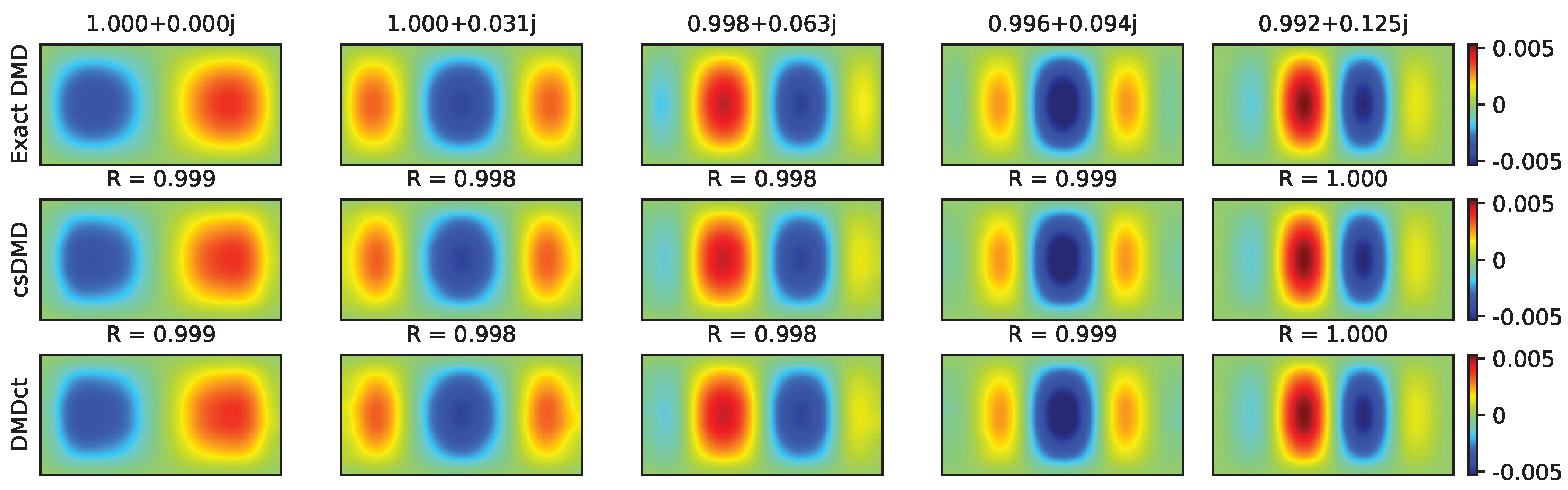
3.1. DMD Mode-Shapes Reconstruction

As the first test, the vorticity of the double-gyre flow (as represented in [10]) was taken and used. The vorticity w is given as

$$\begin{array}{cc}\hfill w=\frac{\partial v}{\partial x}-\frac{\partial u}{\partial y}=& \pi A\cos \left(\pi f(x,t)\right)\sin \left(\pi y\right){\displaystyle \frac{{\partial }^{2}f}{\partial x^2}}-{\pi }^{2}A\sin \left(\pi f(x,t)\right)\sin \left(\pi y\right){\left({\displaystyle \frac{\partial f}{\partial x}}\right)}^2\hfill \\ & -{\pi }^{2}A\sin \left(\pi f(x,t)\right)\sin \left(\pi y\right)\hfill \end{array}$$

(18)

where $A=0.1$, $\omega =\frac{2\pi }{10}$, $ϵ=0.25$, and

$$f(x,t)=ϵ\sin \left(\omega t\right)x^2+x-2ϵ\sin \left(\omega t\right)x$$

(19)

The equation was evaluated over the bounded region $[0,2]\times [0,1]$ for 10 s with time intervals of 0.05 s which resulted in 201 snapshots. The region was discretized as a $512\times 256$ mesh. The number of sampling points was 2500 and they were randomly spread over the region. The same sampling mask was used for both methods. Due to the very few numbers of nonzero Fourier coefficients, only 10 DCT basis vectors along each spatial direction were used ($s_x=s_y=10$). The csDMD method directly resulted in the reconstruction of DMD mode shapes whereas DMDct resulted in the reconstruction of the fully-sampled dataset. After the fully-sampled dataset was reconstructed by DMDct, the exact DMD method was applied to get the DMD mode shapes which were further used for comparison.

All DMDs were performed with nine modes. Since the complex eigenvalues come in pairs of conjugate numbers, only those having non-negative imaginary parts are represented here. Note that, similar to an eigenvector, a mode shape may be multiplied by any non-zero scalar without making a difference. Thus, to compare the mode shapes, they should be aligned with each other prior to making any comparison. Given ${\mathbf{\varphi }}_i$ and ${\mathbf{\psi }}_i$ are the vectorized mode shapes corresponding to the i-th eigenvalue resulted from DMD and csDMD, respectively, the complex scalar $c_i$ that results in the best alignment of the vector ${\mathbf{\psi }}_i$ with the vector ${\mathbf{\varphi }}_i$ is found by solving the following minimization problem

$$c_i=\underset{c}{\mathrm{argmin}}{∥{\mathbf{\varphi }}_i-c{\mathbf{\psi }}_i∥}_2^2=\frac{{\mathbf{\varphi }}_i^T{\overline{\mathbf{\psi }}}_i}{{\mathbf{\psi }}_i^T{\overline{\mathbf{\psi }}}_i}$$

(20)

Similarly, for the vectorized mode shape ${\mathbf{\theta }}_i$ resulted from DMDct, the alignment factor $d_i$ is found as

$$d_i=\underset{d}{\mathrm{argmin}}{∥{\mathbf{\varphi }}_i-d{\mathbf{\theta }}_i∥}_2^2=\frac{{\mathbf{\varphi }}_i^T{\overline{\mathbf{\theta }}}_i}{{\mathbf{\theta }}_i^T{\overline{\mathbf{\theta }}}_i}$$

(21)

Thus, the comparison was made between the vectors ${\mathbf{\varphi }}_i$ and the corresponding aligned vectors $c_i{\mathbf{\psi }}_i$ and $d_i{\mathbf{\theta }}_i$.

Figure 2 shows the real parts of the mode shapes of the first five DMD modes related to the eigenvalues with non-negative imaginary parts and the reconstruction of their mode shapes. The top row shows the mode shapes obtained by applying exact DMD on the fully-sampled dataset, whereas the second and third rows show the aligned csDMD and DMDct reconstructions, respectively. Each column is titled with the corresponding eigenvalue. Both csDMD and DMDct resulted in the reconstruction of the mode shapes with correlation coefficients of approximately 1 which means the reconstructed mode shapes almost identically resembled the references.

Five sample snapshots of the fully-sampled dataset reconstruction are shown in Figure 3. Both methods resulted in reconstruction RMSE of 0.002. The top row of Figure 3 shows the reference snapshots. The samples are shown in the second row. The third and fourth rows show the reconstruction of csDMD and DMDct, respectively.

3.2. Dynamic Denoising and Reconstruction

As the second test, the unforced Duffing equation taken from [7] was used to generate the test dataset. The governing differential equation is

$$\ddot{x}=-\delta \dot{x}-x(\gamma +\alpha x^2)$$

(22)

where $\delta =0.5$, $\gamma =-1$, and $\alpha =1$. The equation was solved over the region $x,\dot{x}\in [-2,2]$, which was discretized as a $41\times 41$ mesh. For each node of the mesh, the corresponding values of x and $\dot{x}$ were taken as the initial conditions and the ODE was solved for 5 s during which the snapshots were taken every 0.1 s resulting in a total of 51 snapshots. Even though the numerical solution resulted in both x and $\dot{x}$ values, only x values were taken and used as the test dataset. 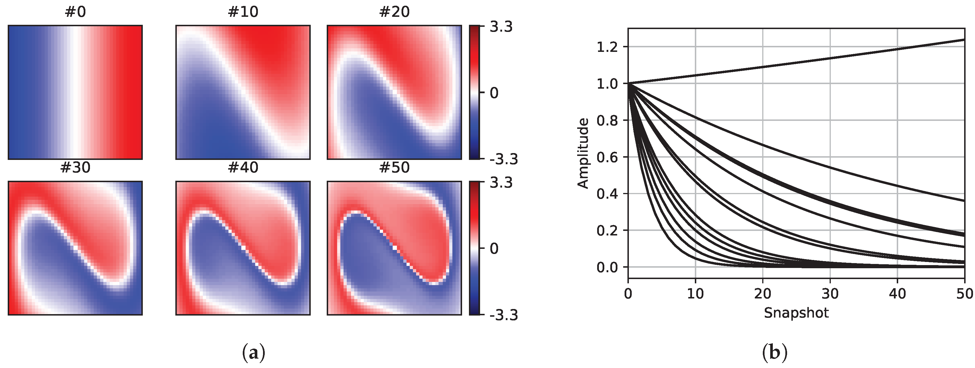Figure 4 shows six sample snapshots of the reference dataset.

Two cases are presented here for comparison. The first case does not have a gap, whereas the second case has a rectangular gap. Both cases were evaluated with noise-free and noisy samples. In all cases, 20% of the available data of each snapshot were taken as the measurement samples and were used for reconstruction. For each case, twenty different random sampling masks were tested. For each mask, the sampling locations remained the same over all snapshots.

The noisy cases were to study the effect of measurement noise and to see how well the two methods could denoise the data. To make the noisy dataset, random Gaussian noise with the standard deviation of 0.25 was added to the reference dataset. The PVNR metric was calculated only for the noisy reconstructions. The same set of basis vectors was used by both methods. For the noise-free samples, the maximum number of basis vectors were used ($s_x=s_y=41$), whereas, for the noisy samples, a reduced set of basis vectors was incorporated ($s_x=s_y=20$), hence dropping the high-frequency components from reconstruction. The eigenvalues derived by csDMD were used for DMDct reconstruction as well. The number of DMD modes to use was found through the method of singular value hard thresholding (SVHT) [22]. According to SVHT, the number of DMD modes for the noise-free and noisy samples was taken as 25 and 5, respectively. Figure 4b shows the amplitudes of the dynamic mode shapes of the reference Duffing dataset. In the figures depicting the snapshots, the first (#0), the middle (#25), and the last (#50) snapshots of the first sampling mask are presented for comparison.

The csDMD method aims at reconstructing the mode shapes and not the fully-sampled dataset. Since no fully-sampled snapshot is available, it is not possible to reconstruct the whole dataset solely based on Exact DMD framework by simply marching forward/backward in time using Equation (2). One possible workaround is to find the optimal amplitudes of DMD modes by minimizing the RMS of reconstruction error as proposed in [6] which leads to

$${\mathbf{b}}_{opt}={\left(\left({\mathsf{\Phi }}_s^{*}{\mathsf{\Phi }}_s\right)\otimes \left(\overline{\mathbf{V}{\mathbf{V}}^{*}}\right)\right)}^{-1}\overline{\mathrm{diag}\mathbf{V}{\mathbf{Z}}^{*}{\mathsf{\Phi }}_s}$$

(23)

where ${\mathsf{\Phi }}_s$ is the matrix of mode shapes as reconstructed by csDMD but only the rows corresponding to the sampled points are kept. Then, the fully-sampled dataset can be reconstructed in full as

$${\tilde{\mathbf{Z}}}_{cs}=\mathsf{\Phi }\mathrm{diag}{\mathbf{b}}_{opt}\mathbf{V}$$

(24)

Equation (24) was used for csDMD reconstruction.

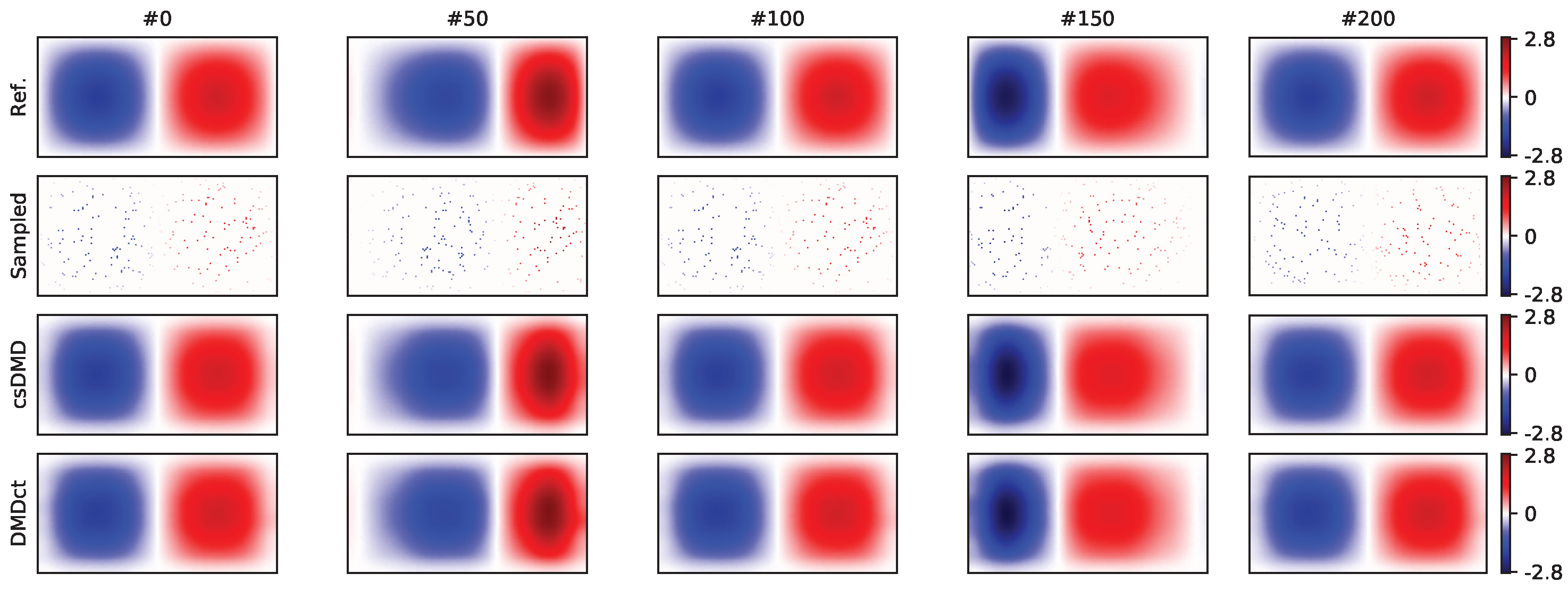
3.3. No-Gap Reconstruction

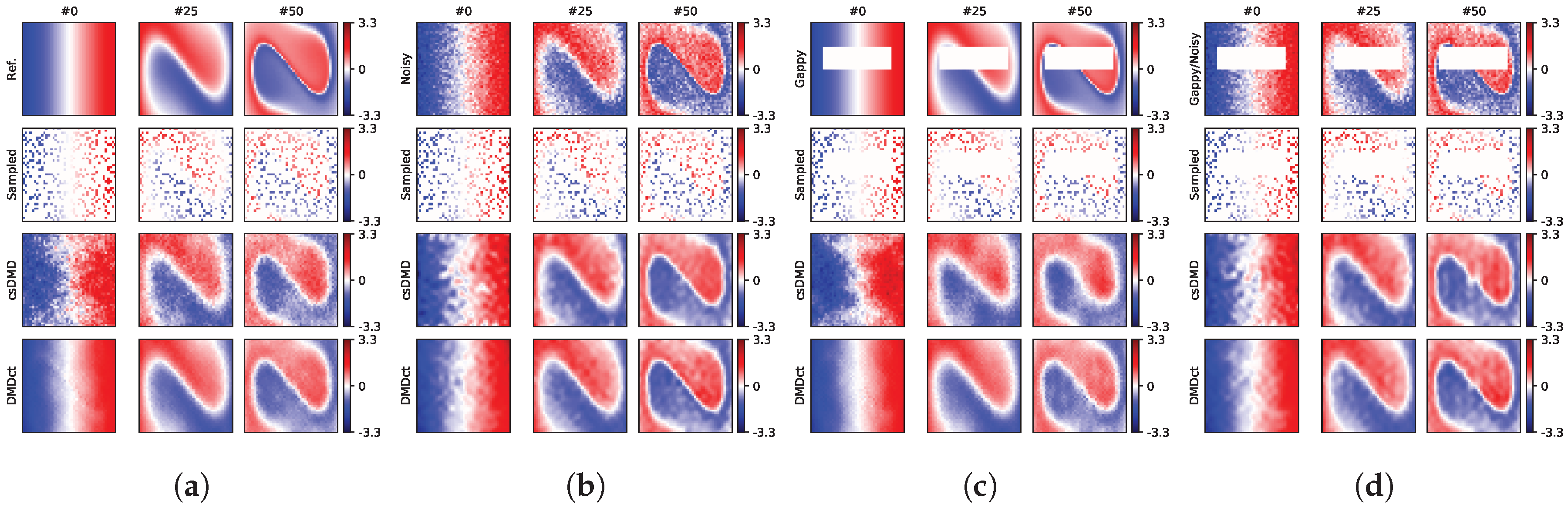
In this case, the reference dataset without any gap was reconstructed by using the two methods. Figure 5a,b, respectively, shows the sample snapshots of the noise-free and noisy reconstructions for the first sampling mask. The noisy dataset had the total PVNR of 19.0 dB and RMSE of 0.250, as depicted in the top row of Figure 5b. In Figure 5a, the top row shows the reference and the second row shows the sampling mask. The third row shows the sample noise-free snapshots as reconstructed by csDMD method resulting in an RMSE value of 0.291. The bottom row shows the same snapshots as reconstructed by DMDct method. The RMSE value of DMDct reconstruction is 0.130. In Figure 5b, the third row shows the results obtained from csDMD method by using the noisy samples. This resulted in an RMSE value of 0.182 and PVNR of 21.8 dB. The bottom row shows the results of DMDct reconstruction which resulted in an RMSE value of 0.119 and PVNR of 25.5 dB.

3.4. Rectangular Gap Reconstruction

For the second case, a rectangular gap was made in the dataset, as shown in the top rows of Figure 5c,d. The size of the gap was $30\times 10$ with the bottom-left and top-right corners at $(-1.5,0)$ and $(1.5,1)$, respectively. The gap covers almost 18% of the area of the region. The first row of Figure 5a shows the reference without the gap, which is what both methods were aimed at recovering by filling the gap. The second row shows the noise-free and noisy samples taken by using the first random sampling mask. The third row shows the reconstruction of csDMD method with corresponding RMSE values of 0.334 for the noise-free samples and 0.181 for the noisy samples. The bottom row shows the reconstruction of DMDct method, where the RMSE values were found as 0.154 and 0.138 for the noise-free and noisy samples, respectively. The respective PVNR values of csDMD and DMDct for the noisy case were 21.8 dB and 24.2 dB. A summary of the error metrics of reconstruction based on the first random sampling mask is presented in

Table 1. The summary of the error metrics for the first random sampling mask. The numbers given are RMSE values with the PVNR values in dB shown inside parenthesis when applicable. In all cases studied, DMDct resulted in lower reconstruction error than csDMD.

Type of Gap	Region	Noise-Free		Noisy
		csDMD	DMDct	Dataset	csDMD	DMDct
None	whole	0.291	0.130	0.250	0.182	0.119
				(19.0 dB)	(21.8 dB)	(25.5 dB)
Rectangular	inside	0.408	0.199	-	0.231	0.185
	outside	0.316	0.142	-	0.168	0.126
	whole	0.334	0.154	0.250	0.181	0.138
				(19.1 dB)	(21.8 dB)	(24.2 dB)

for comparison.

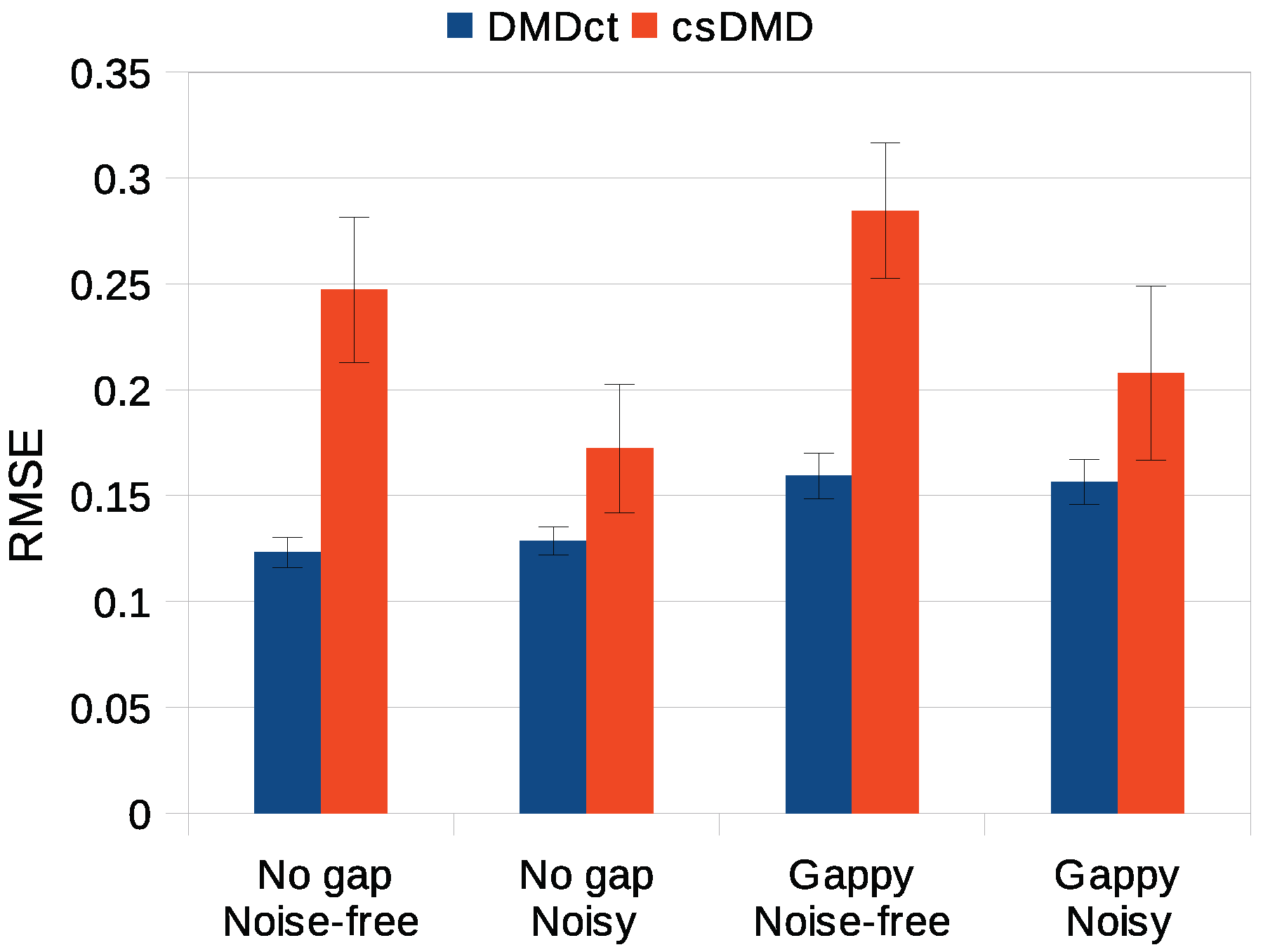
3.5. Statistical Analysis

Three-factor analysis of variance was conducted to determine whether the reconstruction error significantly changed with the three factors method, noise, gap, and their interaction. The RMSE was taken as the error metric and the significance level of 0.05 was used. Tukey post hoc analysis was used for desired pairwise comparisons of significant factors. In all four cases, the two methods were found to result in significantly different reconstruction errors (Tukey post hoc test, $p<0.001$) with the DMDct method having lower error. The effect of noise on DMDct was insignificant ($p=0.797$), whereas the error of csDMD for noisy cases was significantly lower than its error for the noise-free cases ($p<0.001$). Both methods resulted in significantly higher errors for the gappy cases ($p<0.001$). Figure 6 shows the mean RMSE values of DMDct and csDMD for the four test cases studied with the error bars showing the standard deviations.

3.6. Variation of Parameters

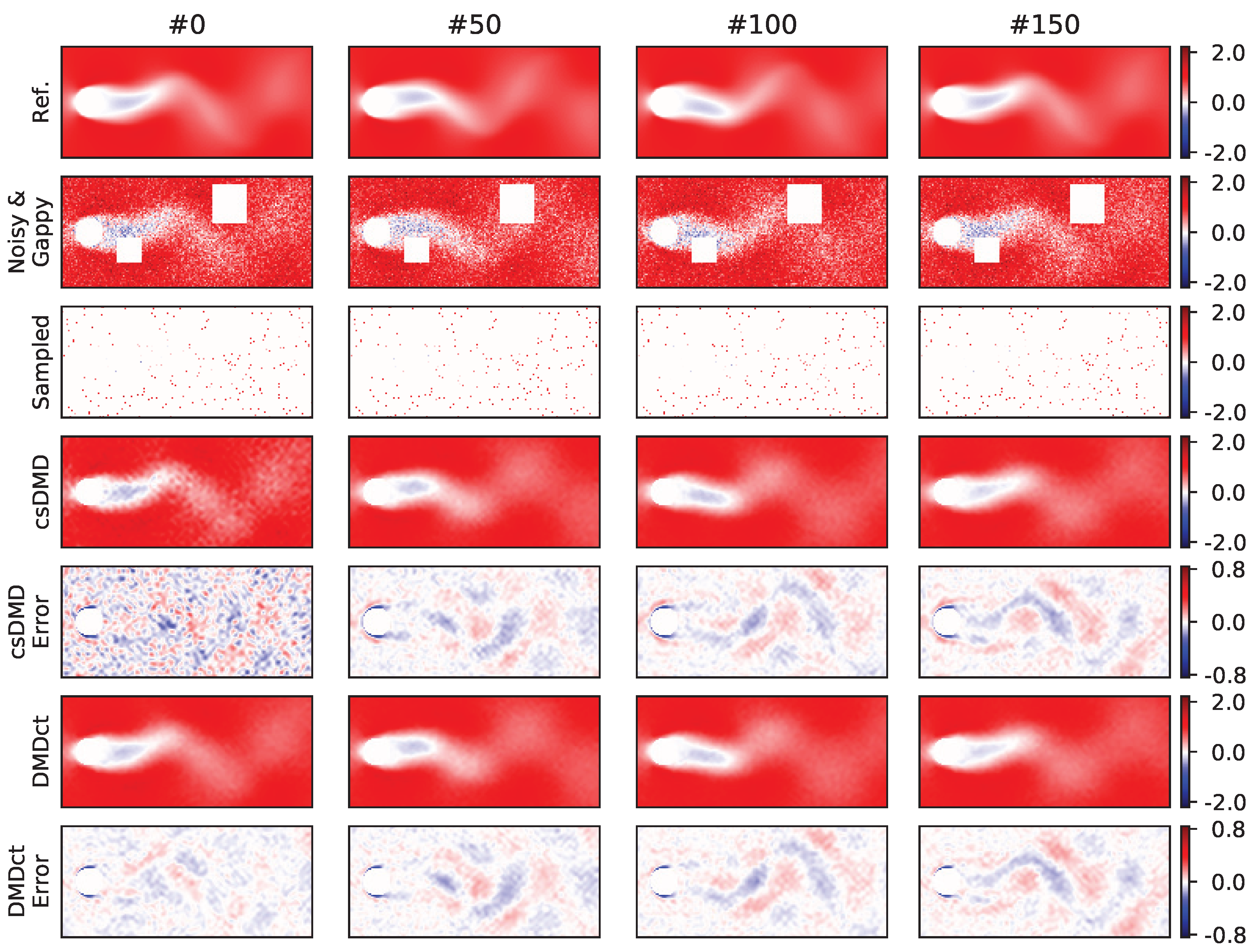
As the third test, a dataset representing the 2-D velocity field for the wake behind a cylinder at Reynolds number Re = 100 taken from [23] was used. The size of the mesh grid is $449\times 199$. The dataset consists of 151 snapshots with regular time intervals of 0.2 s. Random Gaussian noise with a known standard deviation was added to both components. Two rectangular gaps were made in the dataset. The size of the first gap was $60\times 70$ with the bottom-left and top-right corners at $(270,115)$ and $(329,184)$, respectively. The size of the second gap was $46\times 46$ with the bottom-left corner at $(97,44)$ and the top-right corner at $(142,89)$. The aim of this test was to investigate the effect of changing various parameters on the quality of reconstruction. The parameters are noise standard deviation, sampling ratio, number of basis vectors, and number of dynamic modes. The nominal values of the parameters were chosen as noise standard deviation of 0.25, 2% sampling, $s_x=67,s_y=30$, and five dynamic modes (according to SVHT). Although both u and v velocity components were used for analysis, only the results corresponding to the u component are presented here. Figure 7 shows four sample snapshots of the reference noise-free u velocity components, the reference with noise added, the random sample, reconstructions of csDMD and DMDct, and reconstruction errors for the nominal values of the parameters.

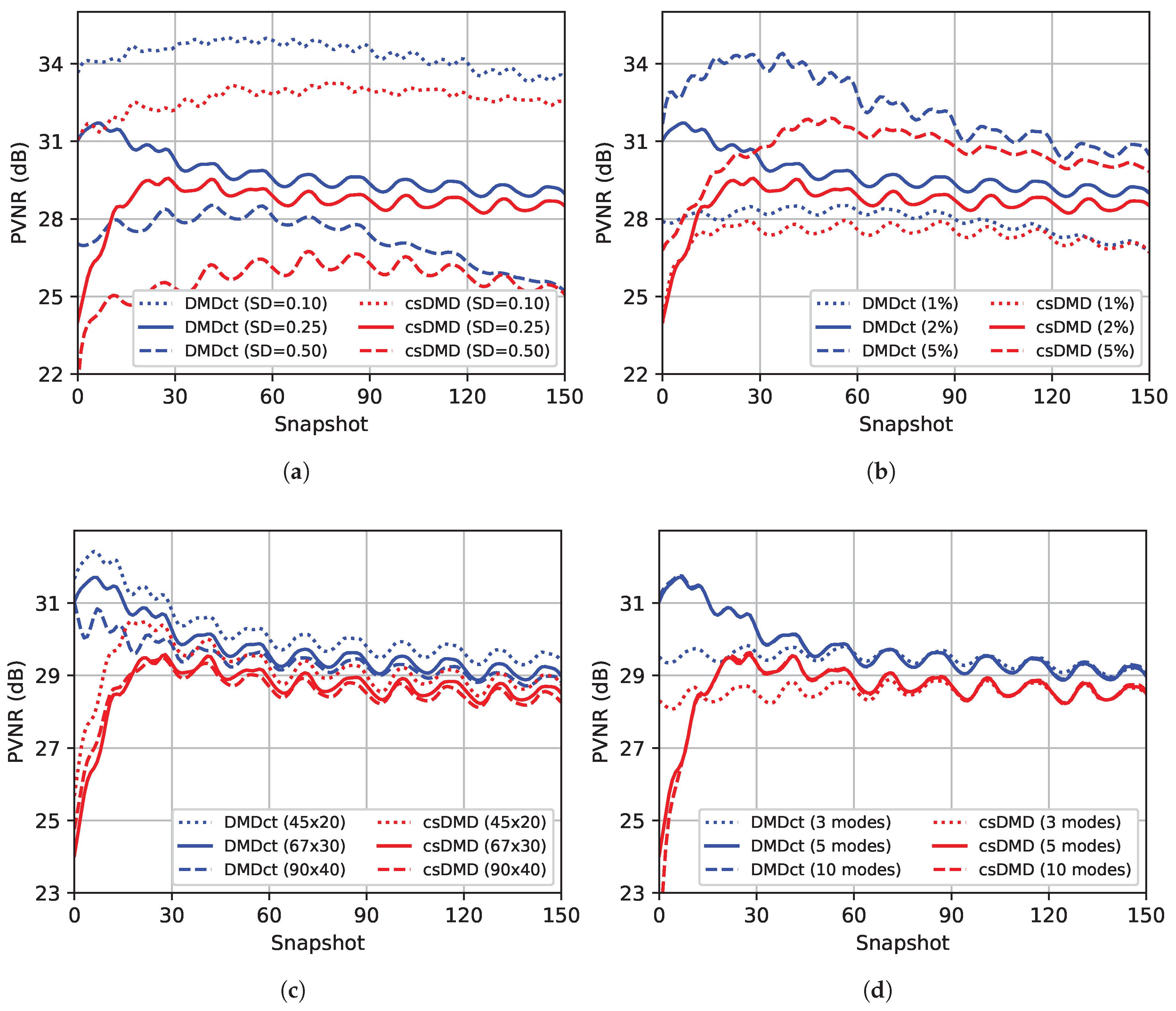
Figure 8 shows the effects of the variation of parameters on PVNR values of csDMD and DMDct reconstructions per snapshot. In all sub-figures, the blue and red curves correspond to DMDct and csDMD results, respectively. The solid lines represent the results based on the nominal values. Figure 8a shows the effect of changing noise standard deviation. As the noise standard deviation increases, the PVNR values drop but in all snapshots, DMDct results in higher PVNR values than csDMD. The effect of changing the sampling ratio is shown in Figure 8b. As expected, increasing the sampling ratio results in higher PVNR values. Figure 8c shows the effect of taking different numbers of basis vectors. As the number of basis vectors increases, the PVNR values drop slightly. Finally, the effect of changing the number of dynamic modes is shown in Figure 8d. Picking a fewer number of modes than SVHT’s result slightly lowers the PVNR values, whereas picking more modes does not make any improvements. The curves corresponding to 5 and 10 modes are almost always overlapping. In all cases studied here, DMDct resulted in higher PVNR values than csDMD in all snapshots.

4. Discussion

The three tests performed aimed at comparing DMDct vs csDMD in terms of both dynamic mode shape reconstruction and fully-sampled dataset reconstruction based on a sparsely-sampled dataset. While csDMD is developed to reconstruct the mode shapes, DMDct reconstructs the fully-sampled dataset. To use csDMD for fully-sampled dataset reconstruction, the spDMD method was incorporated to find the optimal amplitudes of DMD modes.

The first test showed both methods reconstructed the mode shapes almost identical to the ones resulting from applying exact DMD on the fully-sampled dataset even though a very small set of basis vectors was used. Both methods resulted in RMSE of 0.002 in reconstructing the fully-sampled dataset. These results show neither method outperforms the other in dealing with the test dataset which has a few dynamic modes.

The second test consisted of four cases. In the first case, where there is no gap in the data and the samples are noise-free, csDMD reconstruction shows some glitches, especially in the first snapshot, whereas the DMDct reconstruction has much fewer glitches (Figure 5a). The glitches reduce as the time goes on which is probably due to the high decay rate of the corresponding modes. As depicted in Figure 4b, the amplitudes of about half of the modes reduce to 10% or less of their initial values after 20 snapshots which means the corresponding modes die out quickly. In the third and fourth cases, where there is a rectangular gap in the data, DMDct has resulted in less reconstruction error than csDMD in both noisy and noise-free cases. Obviously, the RMSE values are higher compared to those of the no-gap case. Visually comparing, both methods were able to fill the rectangular gap but DMDct seems to have resulted in a smoother and more consistent filling than csDMD. This is also confirmed numerically for the first sampling mask through the RMSE values listed in row “inside” of Table 1.

As the statistical analysis showed, the RMSE values of DMDct reconstruction are significantly lower than those of csDMD. The post hoc analysis also showed the noise has no significant effect on the error of DMDct. This means DMDct is robust with respect to the noise. The glitches in the noisy reconstruction of csDMD seem to be less than the noise-free case, which is probably due to the smaller number of DMD modes taken (5 vs. 25) and the fewer basis vectors used (20 vs. 41). It is also seen DMDct has resulted in more reconstruction error for the noisy cases than the noise-free cases which is as expected, but the reconstruction errors of csDMD for the noisy cases are less than those of the noise-free cases, which indicates csDMD is more sensitive to the number of mode shapes and basis vectors than DMDct.

As stated earlier, the noisy reconstructions were performed using a fewer number of DMD modes and basis functions than the noise-free ones. Comparing the RMSE values in Figure 6 reveals DMDct resulted in less changes in the RMSE values compared to csDMD. In addition, the standard deviation of DMDct results is much lower than csDMD’s according to the error bars in Figure 6. Thus, DMDct is more robust than csDMD.

The third test showed the effect of changing the values of various parameters on the PVNR values of DMDct and csDMD reconstructions. The first parameter to investigate was the standard deviation of the random Gaussian noise. As shown in Figure 8a, as the standard deviation increases, the PVNR values drop which is as expected since higher noise standard deviation means a lower signal-to-noise ratio. For the case of high noise (SD = 0.50), csDMD resulted in a very low PVNR value (<10 dB) in all snapshots (not shown in the figure). This was even lower than the PVNR values of the noisy dataset which means csDMD failed to denoise the data in that case. The second parameter was the sampling ratio. Figure 8b shows higher sampling ratio results in higher PVNR and so, better reconstruction. This is expected as well since higher sampling ratio means more information is provided. In contrast to the first and second cases, the results of changing the number of basis vectors are interesting and unexpected. As shown in Figure 8c, the highest PVNR values correspond to the case of the fewest number of basis vectors ($45\times 20$). We initially expected to observe an improvement in the results as the number of basis vectors increased which did not happen. The reason is that the number of unknowns is determined by the number of basis vectors, i.e., for the case of $45\times 20$ basis vectors, there is a total of 900 unknowns, whereas, for the case of $90\times 40$ basis vectors, the number of unknowns is 3600. Increasing the number of unknowns affects the performance of the $l_1$-regularization method and makes it more difficult to find the proper non-zero subset of coefficients. Thus, limiting the number of basis vectors to a reasonable value is the key. The last parameter to study was the number of dynamic modes. The SVHT method suggested five dynamic modes to pick. Picking fewer modes than five resulted in lower PVNR values over the first half of the snapshots, whereas picking more modes did not make any improvement. This shows the number of modes resulted from SVHT is a good choice.

In all cases studied, the PVNR values of csDMD over the first few snapshots were too low whereas DMDct resulted in less deviation of PVNR values than csDMD. In addition, in all cases, DMDct almost always resulted in higher PVNR values than csDMD.

Even though DMDct was developed for the special case of 2-D problems defined over a rectangular grid of equally-spaced nodes, the method can be extended to the 3D problems as well. It is also possible to adapt the method to an arbitrary grid of nodes.

In summary, DMDct outperforms csDMD in terms of reconstructing the whole dataset regarding the defined metrics. One disadvantage of DMDct compared to csDMD is the more computation time it needs. This is because there are more data to fit in DMDct than csDMD. Since DMDct aims at reconstructing the whole dataset, the Exact DMD must be employed at the end if the mode shapes are desired. The results of both DMDct and csDMD are sensitive to the value of sparseness coefficient $\beta$ in Equation (13). Here, we ran each algorithm with various $\beta$ values and then picked the best ones for comparison. For a real case, where the actual solution is unknown, this approach is impractical. The proper choice of sparseness coefficient $\beta$ remains an open question and will be addressed later.

5. Conclusions

In this paper, a novel approach for dynamic reconstruction of a given dataset based on DMD and a set of basis vectors and by taking a random sub-sample of the fully-sampled dataset is proposed. The proposed approach was compared against csDMD in terms of reconstruction error for three test cases. The results of the tests show that, while the two methods performed similarly on the dataset with a few number of dynamic modes, the proposed method outperformed csDMD in terms of both denoising and gap-filling. The third test also showed per-snapshot reconstruction error of DMDct has less variation than csDMD reconstruction.