Lattice Boltzmann Simulation of Immiscible Two-Phase Displacement in Two-Dimensional Berea Sandstone

Abstract

Understanding the dynamic displacement of immiscible fluids in porous media is important for carbon dioxide injection and storage, enhanced oil recovery, and non-aqueous phase liquid contamination of groundwater. However, the process is not well understood at the pore scale. This work therefore focuses on the effects of interfacial tension, wettability, and the viscosity ratio on displacement of one fluid by another immiscible fluid in a two-dimensional (2D) Berea sandstone using the colour gradient lattice Boltzmann model with a modified implementation of the wetting boundary condition. Through invasion of the wetting phase into the porous matrix, it is observed that the viscosity ratio plays an important role in the non-wetting phase recovery. At the viscosity ratio ($\lambda$) of unity, the saturation of the wetting fluid is highest, and it linearly increases with time. The displacing fluid saturation reduces drastically when $\lambda$ increases to 20; however, when $\lambda$ is beyond 20, the reduction becomes less significant for both imbibition and drainage. The front of the bottom fingers is finally halted at a position near the inlet as the viscosity ratio increases to 10. Increasing the interfacial tension generally results in higher saturation of the wetting fluid. Finally, the contact angle is found to have a limited effect on the efficiency of displacement in the 2D Berea sandstone.

1. Introduction

The simultaneous flow of two immiscible fluids in porous media is often found in nature and industrial processes such as non-aqueous phase liquid (NAPL) contamination of groundwater, carbon dioxide injection and storage, and enhanced oil recovery (EOR) operations. For the spontaneous imbibition of oil, carbon dioxide or water, which is immiscible to the oil phase, is usually imbibed into permeable rock formations which are characterized by low porosity and low in situ permeability. The displacement process is affected by matrix properties such as the heterogeneity, wettability, and fluid properties of each phase [1].

Experimental efforts have been made to understand interactions between fluids and rock during fluid displacement [2,3]. Theoretical works usually use simplified pore geometries which allow theoretical solutions to the microscopic flow patterns [4]. As a complementary method to the experimental and theoretical approaches, accurate and reliable numerical tools are needed to understand the underlying mechanisms of multiphase displacement. Conventional macro-scale simulations have achieved great success in solving the continuity, momentum, and species balance equations which rely on the empirical estimation of relative permeabilities. This approach, however, may not be able to capture effects related to micro-scale structure in a multiphase system. On the contrary, pore-scale simulation can provide local detailed information about the flow field. The previous works on pore-scale simulation of immiscible two-phase flows in porous media [5,6,7,8,9,10] have been shown to be capable of capturing the effects of various factors, e.g., capillary number, viscosity ratio, surface wettability, and media heterogeneity. However, due to the inherent complexity related to interface evolution, heterogeneous geometry, dominant capillarity, and moving contact line, the computational simulation of multiphase displacement in realistic porous media still remains a research challenge.

As a mesoscopic method, the lattice Boltzmann method (LBM) has been widely accepted as a useful alternative for simulating multiphase flows, in particular, with the advantage of dealing with complex geometries such as porous media [11]. A number of multiphase LBM models have been proposed, e.g., the colour gradient model [12,13], the pseudo-potential model [14], the free energy model [15] and the mean-field model [16]. The colour gradient model is known to be the first multiphase model. Later, a new multiphase LBM model was proposed by Shan and Chen [14], where the interparticle forces (whether attractive or repulsive) mimicking the molecular potentials are introduced by a modified equilibrium velocity in the equilibrium distribution functions. The free energy model is thermodynamically consistent, and it considers a generalised equilibrium distribution function that includes a nonideal pressure tensor term. The original free energy model suffers from a lack of Galilean invariance, but later works have mitigated this problem [17,18]. The mean-field model describes interfacial dynamics based on the mean-field theory, and uses a pressure distribution function instead of its density counterpart to reduce discretization errors in the calculation of density gradient and to improve the numerical stability for variable density. Extensive reviews of these LBM multiphase models can be found in previous research [8,19].

The viscosity contrast is large while the density difference is small for the water or carbon dioxide involved oil recovery process. However, most LBM models can only access a limited range of viscosity ratios for dynamic fluid displacement. Yang et al. [20] performed a systematic comparison of three popular multiphase models, i.e., the pseudo-potential model, the free energy model, and the colour gradient model, for flow simulations in porous media. They concluded that the pseudo-potential model is a promising tool for liquid-gas systems, but may not be the optimal solution for the simulation of immiscible flows. Also, it produces high spurious velocities and thick interfaces for immiscible flows [20]. Jonathan et al. [21] used the pseudo-potential model to simulate two-phase flows in a two-dimensional channel with different viscosity ratios. A viscous-fingering-like phenomenon was observed for viscosity ratios of up to 10, and the simulations become unstable for larger viscosity ratios. Hatiboglu et al. [22] studied the spontaneous imbibition of water into a water-wet micro-model which was initially saturated with oil. It was verified that the maximum allowable viscosity ratio is four. The free energy model and colour gradient model show similar capabilities in modelling the flow of binary fluids with high viscosity contrast, but the latter produces a relatively thinner interface than the former one. In addition, the colour gradient model is able to control the interfacial diffusion and adjust the interfacial tension and viscosity independently to facilitate the numerical investigation.

The colour gradient LBM was first proposed by Rothman and Keller [13], and has been widely used for the simulation of immiscible fluids [9,12,23,24,25,26]. To obtain an accurate and detailed understanding of the pore-scale mechanisms within porous media, Xu et al. [25] proposed a new algorithm for imposing the contact angle on the solid surface in the colour gradient LBM. The simulation results were validated against the experimental observations of Wu et al. [27]. However, these simulations only dealt with the simplified porous media, where the solid grains are regular circles and rectangles. In realistic porous media, the pore structures are extremely complex and irregular, which allow us to further assess the capability of numerical model. We apply the colour gradient LBM for dynamic displacement of immiscible fluids in a complex porous flow structure extracted from a realistic Berea sandstone sample, and study the effects of the viscosity ratio, interfacial tension, and contact angle on displacement process.

2. Colour Gradient Lattice Boltzmann Model for Two-Phase Flow

The colour gradient LBM was used in this work. In this model, the “Red” and “Blue” distribution functions ($f_i^R$ and $f_i^B$) are used to represent two different fluids. The total distribution function is defined as $f_i=f_i^R+f_i^B$. Each colored distribution function undergoes the collision and streaming steps expressed by the following equation:

$$f_i^k(\mathit{x}+{\mathit{c}}_i\Delta t,t+\Delta t)=f_i^k(\mathit{x},t)+{\mathsf{\Omega }}_i^k\left(f_i^k(\mathit{x},t)\right),$$

(1)

where $\mathit{x}$ and t are the position and time, k = red or blue, i represents the discrete velocity directions for the two-dimensional 9-velocity (D2Q9) model, $\Delta t$ is the time step, and ${\mathit{c}}_i$ denotes the lattice velocity vectors in the i-th discrete velocity direction. For the two-dimensional 9-velocity (D2Q9) model used in this work, the lattice velocity vector is given by

$${\mathit{c}}_i=\left\{\begin{array}{cc}(0,0),\hfill & i=0\hfill \\ \left(\cos \right[\pi (i-1)/2],\sin [\pi (i-1)/2\left]\right),\hfill & i=1,2,3,4\hfill \\ \sqrt{2}(\cos [\pi (i-5)/2+\pi /4],\sin [\pi (i-5)/2+\pi /4]),\hfill & i=5,6,7,8.\hfill \end{array}\right.$$

(2)

The collision step includes self- and cross-interactions with the other type of particles which can be written as

$${\mathsf{\Omega }}_i^k={\left({\mathsf{\Omega }}_i^k\right)}^{\left(3\right)}\left[{\left({\mathsf{\Omega }}_i^k\right)}^{\left(1\right)}+{\left({\mathsf{\Omega }}_i^k\right)}^{\left(2\right)}\right],$$

(3)

where ${\left({\mathsf{\Omega }}_i^k\right)}^{\left(1\right)}$ is the single-phase collision operator, ${\left({\mathsf{\Omega }}_i^k\right)}^{\left(2\right)}$ is the perturbation operator, and ${\left({\mathsf{\Omega }}_i^k\right)}^{\left(3\right)}$ is the recolouring operator.

2.1. Single-Phase Collision Operator

To achieve high accuracy and good stability, we implemented the collision step in accordance with the two-relaxation-time (TRT) model [28,29,30]—a special multiple relaxation time (MRT) model with only two relaxation rates [31]. With the TRT model, the single-phase collision operator is expressed as

$${\left({\mathsf{\Omega }}_i^k\right)}^{\left(1\right)}=-{\left({\mathbf{M}}^{-1}\mathbf{S}\mathbf{M}\right)}_{ij}(f_j^k-f_j^{k,eq}),$$

(4)

where $\mathbf{M}$ is the transformation matrix and is given by

$$\mathbf{M}=\left(\begin{array}{ccccccccc}1& 1& 1& 1& 1& 1& 1& 1& 1\\ -4& -1& -1& -1& -1& 2& 2& 2& 2\\ 4& -2& -2& -2& -2& 1& 1& 1& 1\\ 0& 1& 0& -1& 0& 1& -1& -1& 1\\ 0& -2& 0& 2& 0& 1& -1& -1& 1\\ 0& 0& 1& 0& -1& 1& 1& -1& -1\\ 0& 0& -2& 0& 2& 1& 1& -1& -1\\ 0& 1& -1& 1& -1& 0& 0& 0& 0\\ 0& 0& 0& 0& 0& 1& -1& 1& -1\end{array}\right).$$

(5)

The diagonal relaxation matrix $\mathbf{S}$ is defined as

$$\mathbf{S}=(1,s_e,s_{\epsilon },1,s_q,1,s_q,0,s_q,s_{\nu },s_{\nu }).$$

(6)

For the conserved moments of density and momentum, the relaxation rates were set to 1. $s_e$ and $s_{\nu }$ are related to the bulk and shear viscosities, and $s_{\epsilon }$ and $s_q$ are free parameters. Following the recommendations of Ginzburg et al. [32], these relaxation rates were taken as

$$s_e=s_{\epsilon }=s_{\nu }=\frac{1}{\tau },s_q=8\frac{(2-s_{\nu })}{(8-s_{\nu })},$$

(7)

where $\tau$ is the dimensionless relaxation time. The mass conservation for each fluid distribution function and the total momentum conservation require

$${\rho }_k=\sum _i{f}_i^k=\sum _i{f}_i^{k,eq},\rho \mathit{u}=\sum _i\sum _k{f}_i^k{\mathit{c}}_i=\sum _i\sum _k{f}_i^{k,eq}{\mathit{c}}_i,$$

(8)

where $\rho$ is the total density, and ${\rho }_k$ is the density of fluid k, and $\mathit{u}$ is the local fluid velocity.

The equilibrium distribution function ($f_i^{k,eq}(\mathit{x},t)$) is a truncated Taylor series expansion up to the second order in Mach number of the Maxwell–Boltzmann equilibrium distribution function, which was chosen to satisfy Equation (8):

$$f_i^{k,eq}({\rho }_k,\mathit{u})={\rho }_k{W}_i\left[1+\frac{{\mathit{c}}_i·\mathit{u}}{c_s^2}+\frac{{({\mathit{c}}_i·\mathit{u})}^2}{2c_s^4}-\frac{{\mathit{u}}^2}{2c_s^2}\right],$$

(9)

in which, $c_s=1/\sqrt{3}$ is the lattice sound speed, and the weight coefficients are $W_0=4/9$, $W_{1-4}=1/9$ and $W_{5-8}=1/36$ for the D2Q9 lattice model. As we focused on the oil-water two-phase systems, the density ratio of both fluids was set to be unity.

To ensure a constant viscosity across the interface when both fluids were of different viscosities, the following harmonic mean [33] was employed to determine the viscosity of the fluid mixture:

$$\frac{1}{\eta }=\frac{1+{\rho }^N}{2{\eta }_R}+\frac{1-{\rho }^N}{2{\eta }_B},$$

(10)

where ${\eta }_k$ ($k=R$ or B) is the dynamic viscosity of fluid k, and $\eta$ is the dynamic viscosity of the fluid mixture which is related to the dimensionless relaxation time $\tau$ by $\eta =c_s^2\rho (\tau -0.5)\delta t$; ${\rho }^N$ is the indicator function used to distinguish different fluids, and it is defined as

$${\rho }^N(\mathit{x},t)=\frac{{\rho }_R(\mathit{x},t)-{\rho }_B(\mathit{x},t)}{{\rho }_R(\mathit{x},t)+{\rho }_B(\mathit{x},t)}.$$

(11)

2.2. Perturbation Operator

${\left({\mathsf{\Omega }}_i^k\right)}^{\left(2\right)}$ takes effect in the mixed interfacial region to generate an interfacial tension. Using the continuum surface force (CSF) [34] model, a body force term was added to the macroscopic momentum equation, and it reads as

$${\mathit{F}}_s=\frac{1}{2}\sigma K\mathbf{\nabla }{\rho }^N,$$

(12)

where $\sigma$ is the interfacial tension coefficient, and K is the local interface curvature calculated by [34]

$$K=-{\mathbf{\nabla }}_s·\mathit{n},$$

(13)

where ${\nabla }_s=(\mathbf{I}-\mathit{n}\mathit{n})·\mathbf{\nabla }$ is the surface gradient operator, $\mathbf{I}$ is the second-order identity tensor, and $\mathit{n}=\mathbf{\nabla }{\rho }^N/\left|\mathbf{\nabla }{\rho }^N\right|$ is a unit vector normal to the interface. Such a body force was then incorporated into LBM through the forcing scheme proposed by Guo et al. [35] which can significantly improve computation accuracy and reduce spurious velocities effectively [36]. The perturbation operator ${\left({\mathsf{\Omega }}_i^k\right)}^{\left(2\right)}$ is expressed as

$${\left({\mathsf{\Omega }}_i^k\right)}^{\left(2\right)}={\mathbf{M}}^{-1}(\mathbf{I}-\frac{1}{2}\mathbf{S}){\mathit{F}}^k,$$

(14)

with

$$\begin{array}{cc}\hfill {\mathit{F}}^k(\mathit{x},t)& ={\alpha }_k[0,6(u_x{F}_{sx}+u_y{F}_{sy}),\hfill \\ & -6(u_x{F}_{sx}+u_y{F}_{sy}),F_{sx},-F_{sx},F_{sy},-F_{sy}\hfill \\ & 2(u_x{F}_{sx}-u_y{F}_{sy}),u_x{F}_{sy}+u_y{F}_{sx}{]}^T,\hfill \end{array}$$

(15)

where ${\alpha }_k$ is the fraction of interfacial tension contributed by fluid k and satisfies ${\sum }_k{\alpha }_k=1$.

The fluid velocity was corrected to recover the Navier–Stokes (N-S) equations in the interfacial region where two fluids coexist

$$\rho \mathit{u}=\sum _i\sum _k{f}_i^k{\mathit{c}}_i+\frac{1}{2}{\mathit{F}}_s.$$

(16)

2.3. Recolouring Operator

The recolouring step was then applied to promote phase segregation and maintain a sharp interface [37] which is given as

$${\left({\mathsf{\Omega }}_i^R\right)}^{\left(3\right)}=\frac{{\rho }_R}{\rho }{f}_i^{\ast }+\beta \frac{{\rho }_R{\rho }_B}{{\rho }^2}{f}_i^{\left(eq\right)}(\rho ,\mathit{u}=0)\cos \left({\phi }_i\right),$$

(17)

$${\left({\mathsf{\Omega }}_i^B\right)}^{\left(3\right)}=\frac{{\rho }_B}{\rho }{f}_i^{\ast }-\beta \frac{{\rho }_R{\rho }_B}{{\rho }^2}{f}_i^{\left(eq\right)}(\rho ,\mathit{u}=0)\cos \left({\phi }_i\right),$$

(18)

where $f_i^{\ast }={\sum }_k{f}_i^{k\ast }$ denotes the post-perturbation, pre-segregation value of the total distribution function along the i-th discrete velocity direction, and $f_i^{eq}={\sum }_k{f}_i^{k,eq}$ is the total equilibrium distribution function. $\beta$ is the segregation parameter related to the interface thickness, and its value must be between 0 and 1 to ensure positive particle distributions—it was chosen to be 0.7 here. ${\phi }_i$ is the angle between the indicator function gradient $\mathbf{\nabla }{\rho }^N$ and the lattice vector ${\mathit{c}}_i$, which is defined by

$$\cos \left({\phi }_i\right)=\frac{{\mathit{c}}_i·\mathbf{\nabla }{\rho }^N}{|{\mathit{c}}_i\left|\right|\mathbf{\nabla }{\rho }^N|}.$$

(19)

To minimize the discretization error, a fourth-order isotropic finite difference was used to calculate the partial derivatives. For example, for a variable $\psi$, the partial derivatives can be calculated by

$$\mathbf{\nabla }\psi (\mathit{x},t)=\frac{1}{c_s^2}\sum _i{W}_i\psi (\mathit{x}+{\mathit{c}}_i{\delta }_t,t){\mathit{c}}_i.$$

(20)

2.4. Wetting Boundary Condition

For the colour gradient LBM, the most widely-used wetting boundary condition is to set a virtual density at solid surfaces [37]. However, it has been found in recent works [38,39] that numerical errors resulting from nonphysical mass transfer and spurious velocities may be accumulated during simulations which potentially render meaningless results. To overcome this, the algorithm proposed by Xu et al. [25] was implemented to impose the contact angle on solid surfaces. This algorithm is able to precisely control the contact angle for both static and dynamic problems which is essential for accurate simulations of two-phase displacement in porous media.

3. Relative Permeability Validation: Concurrent Flow in a 2D Channel

We first used the above model to simulate a pressure driven flow through a porous media. In the single-phase case, the intrinsic permeability K can be determined according to the Darcy’s law [4]

$$\mathit{u}=-\frac{K}{\mu }\mathbf{\nabla }P,K=-\frac{\mu \mathit{u}}{\mathbf{\nabla }P},$$

(21)

where $\mathit{u}$ is the Darcy velocity in the porous medium. Note that the intrinsic permeability does not depend on the nature of the flow field but only on the geometry of the porous medium. In case of two-phase flows, the relative permeability $K_{r,i}$ can be given as [4]

$${\mathit{u}}_i=\frac{K{K}_{r,i}}{{\mu }_i}\mathbf{\nabla }{P}_i,K_{r,i}=\frac{{\mu }_i{\mathit{u}}_i}{K\mathbf{\nabla }{P}_i},i=w,nw.$$

(22)

Here, $i=w$ and $nw$ refer to the wetting and non-wetting fluids respectively, ${\mu }_i$ is the dynamic viscosity of fluid i, and $\mathbf{\nabla }{P}_i$ is the pressure gradient of fluid i.

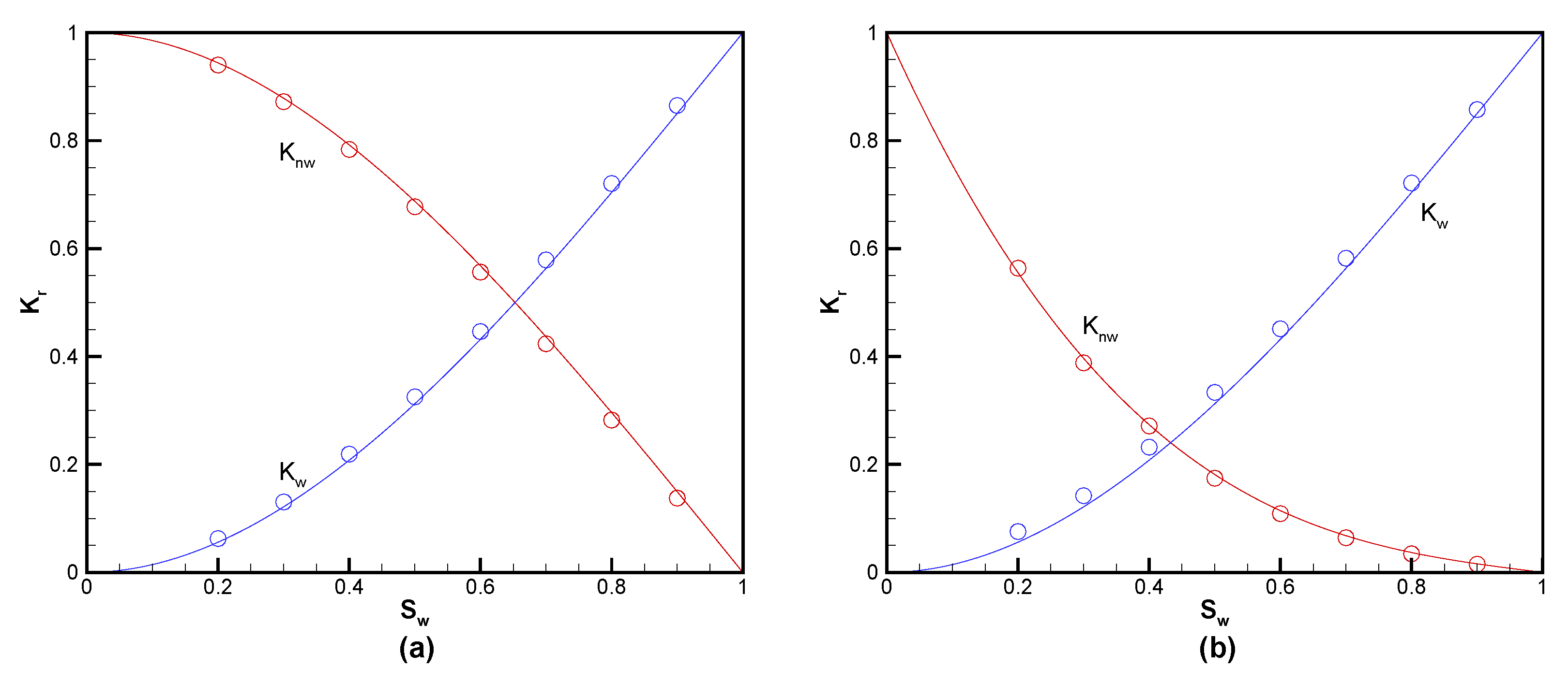
First, we tested whether the LBM model can accurately predict relative permeability for a simple immiscible two-phase cocurrent flow. Specifically, we calculated the relative permeabilities of the layered two-phase flow in a channel under different saturation values. In the simulation, a constant pressure difference was applied on the inlet and outlet boundaries following Zou and He [40], and a non-slip (bounce-back) boundary condition was applied on the upper and lower walls using the halfway bounce-back scheme. The wetting phase flowed along the walls ($a<\left|y\right|\le b$) and non-wetting phase flowed in the central region ($\left|y\right|<a$). One can obtain the analytical solutions for the relative permeability, a function of wetting phase saturation $S_w$ and viscosity ratio $\lambda$ [41],

$$K_{r,nw}=(1-S_w)\left[\frac{3}{2}\lambda +{(1-S_w)}^2(1-\frac{3}{2}\lambda )\right],K_{r,w}=\frac{1}{2}{S}_w^2(3-S_w),$$

(23)

where $S_w$ is the wetting phase saturation, which is defined as $S_w=1-a/b$, and $\lambda$ is the viscosity ratio of the non-wetting to wetting fluids, i.e., $\lambda ={\mu }_{nw}/{\mu }_w$.

For two typical viscosity ratios of $\lambda =1$ and $\lambda =0.1$, Figure 1 shows excellent agreement between the computed relative permeabilities and the analytical solutions.

4. Results and Discussion

This section describes the conduction of a systematic investigation on a pressure-driven immiscible two-phase flow in a 2D micromodel extracted from Boek et al. [42], which was engineered at Schlumberger Cambridge Research based on a thin section of a 3D Berea sandstone rock sample. We defined the lattice units for length, mass and time as lu, ts, and mu, respectively. To match the parameters in the lattice unit towards their physical values, three basic physical quantities were chosen as the reference values: the length scale ($l_0$), the mass scale ($m_0$) and the time scale ($t_0$). In the present study, $l_0=8\times {10}^{-6}$ m, $m_0=5.12\times {10}^{-13}$ kg, and $t_0=7.2\times {10}^{-7}$ s. Therefore, the density can be obtained by ${\rho }^{phy}=\rho \frac{m_0}{l_0^3}=\frac{5.12\times {10}^{-13}}{{(8\times {10}^{-6})}^3}={10}^3$ kg·m${}^{-3}$, the dynamic viscosity by ${{\mu }_{displaced}}^{phy}={\mu }_{displaced}\frac{m_0}{l_0{t}_0}=0.167\times \frac{5.12\times {10}^{-13}}{8\times {10}^{-6}\times 7.2\times {10}^{-7}}=0.0148$ Pa·s, and the interfacial tension by ${\sigma }^{phy}=\sigma m_0/{t_0}^2$. For the interfacial tension values used in the present work, the corresponding physical values for 0.03 mu·ts${}^{-2}$, 0.015 mu·ts${}^{-2}$, and 0.0005 mu·ts${}^{-2}$ were 0.0296 N·m${}^{-1}$, 0.0148 N·m${}^{-1}$, and 0.0004938 N·m${}^{-1}$, respectively.

4.1. Problem Statement

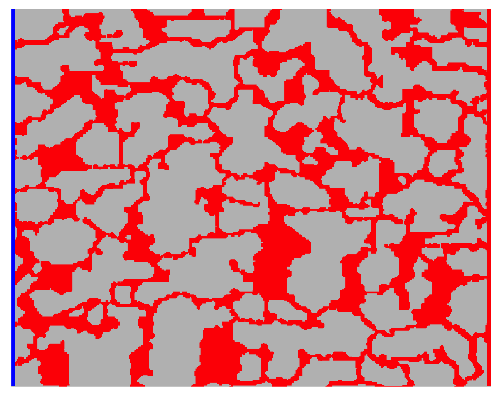
The 2D micromodel is shown in Figure 2, and its porosity is 0.33. The entire micromodel is divided into $L\times H$ = $2644\times 2117$ lu${}^2$ with a resolution of 0.67 $\mathsf{\mu }$m per lu. The narrowest throat has a width of 12 lu which is fine enough to produce grid-independent results in two-phase displacement simulations [7].Twenty-two extra layers of lattices are added to both the inlet and outlet to facilitate the implementation of boundary conditions, so the actual domain size is $2688\times 2117$ lu${}^2$. Here, the flow velocity for each fluid is so small that the inertial effect becomes insignificant.

The constant pressure boundary condition developed by Zou and He [40] was imposed on the inlet and outlet, which are located at the left and right sides of the domain, respectively. The halfway bounce-back scheme and wetting boundary condition were applied at the walls that contain the surfaces of solid grains as well as the upper and lower sides of the domain. The densities of both wetting and non-wetting fluids were set to be unity as the density difference between oil and water is insignificant. The dynamic viscosity of the displaced fluid was kept as 0.167 mu·lu${}^{-1}$·ts${}^{-1}$, and the dynamic viscosity of the displacing fluid was varied to achieve different viscosity ratio values ($\lambda ={\mu }_{displaced}/{\mu }_{invading}$). Initially, for $x\ge 22$ lu, the domain was filled with the displaced fluid (represented in red) at rest, and a constant pressure $p_{out}=1/3$ mu·lu${}^{-1}$·ts${}^{-2}$ was imposed at the outlet, while for $x<22$ lu, the region was occupied by the displacing fluid (represented in blue) with a higher pressure at the inlet. The simulations stopped when the displacing fluid broke through at the outlet to avoid the capillary end effect [43].

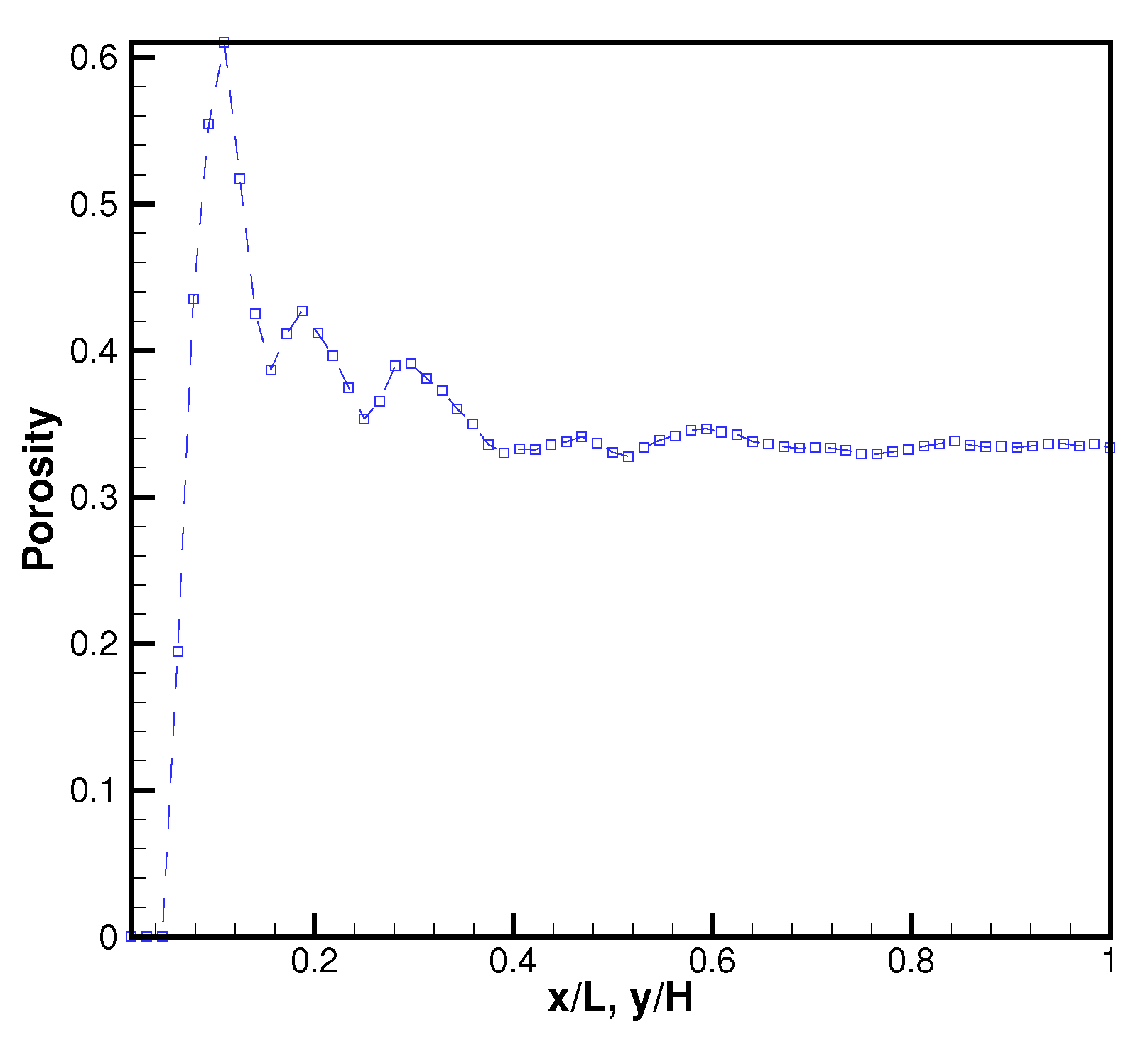
By studying the dependency of porosity on the size of the rock sample, we calculated the porosity using different sizes of Berea sandstone to find its representative elementary volume (REV). The results are shown in Figure 3, which demonstrates that the chosen size of $2688\times 2117$ lu${}^2$ could be a good REV of the Berea sandstone. This guarantees that the simulated geometry included a sufficient number of pores for the meaningful statistical average, which is generally required by the continuum concept [4].

4.2. The Viscosity Ratio Effect

The viscosity ratio is one of the most important dimensionless numbers in two-phase displacement through a porous media, and its effect was studied for a constant contact angle of ${120}^{\circ }$, corresponding to a weak wetting property of the displacing fluid. The inlet pressure is also the same for different viscosity ratios, i.e., $p_{in}=(p_{out}+0.0125)$ mu·lu${}^{-1}$·ts${}^{-2}$. Figure 4 shows the fluid distributions inside the pore network when breakthrough of the displacing fluid occurs for viscosity ratios of 1, 2, 5, and 10. It can be seen that for all the viscosity ratios considered, two or three preferential paths are generally formed. As the viscosity ratio increases, it becomes harder for the finger to flow into the large pore as highlighted by the black elliptical circles. The front of the bottom finger is finally halted at the position near the inlet for the viscosity ratio of 10. Also, the breakthrough finger switches to a lower position at the outlet when the viscosity ratio increases to 10.

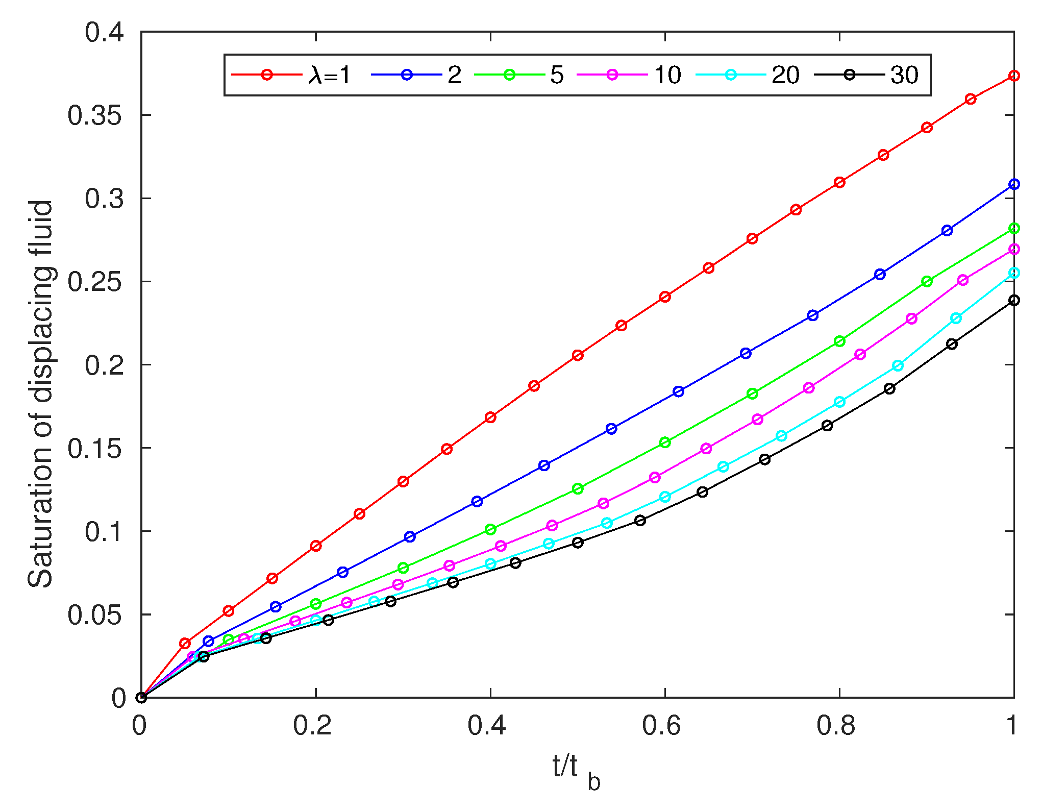
Figure 5 shows the time evolution of the displacing (wetting) fluid saturation for a viscosity ratio changing from 1 to 30. It can be clearly seen that a higher viscosity ratio results in a lower fluid saturation which is less favourable for the recovery of displaced fluid. This is consistent with previous experimental [44] and numerical results [45]. At the viscosity ratio of unity, the highest displacing fluid saturation (around 0.37) is observed, and the displacing fluid saturation keeps increasing linearly with time. Although the displacing fluid saturation reduces with $\lambda$, the reduction becomes less significant at larger $\lambda$ values.

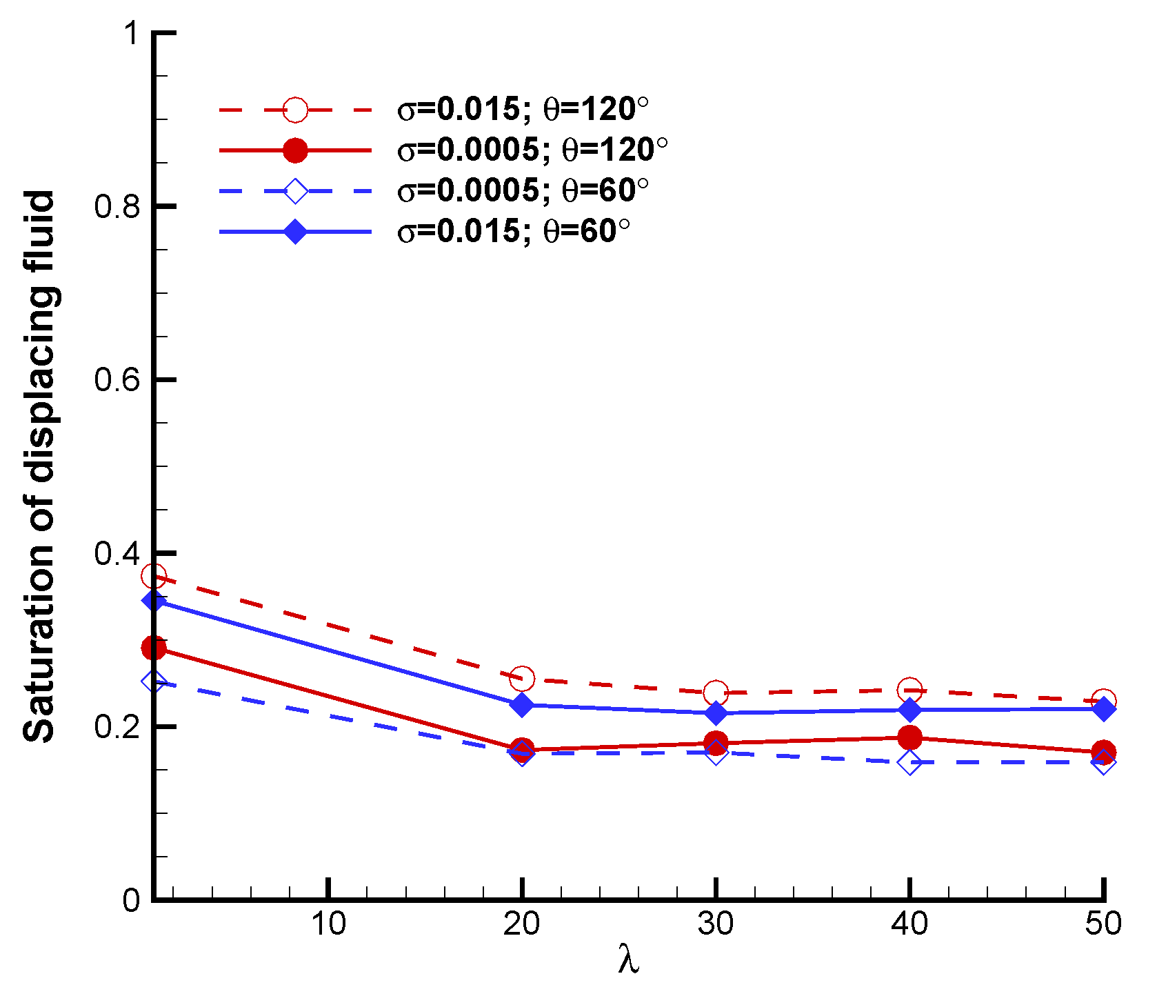
We also tested whether the above observations are valid for varying wettability and interfacial tension. Four pairs of contact angle and interfacial tension were considered (see

Table 1. Parameters used in four typical cases of immiscible displacement.

Case	$\mathbf{\Delta }\mathit{P}$	$\mathit{\sigma }$	$\mathbf{cos}\mathit{\theta }$
I	0.0125	0.015	−0.5
II	0.0125	0.0005	−0.5
III	0.0125	0.0005	0.5
IV	0.0125	0.015	0.5

), and the simulation results are shown in Figure 6. It is clear that the displacing fluid saturation drops rapidly when the viscosity ratio increases from 1 to 20 and then stays almost unchanged for all the cases considered. For each viscosity ratio, increasing contact angle or interfacial tension always leads to a higher displacing fluid saturation or displacement efficiency. In addition, the limitation of the current model was tested by decreasing the viscosity of the displacing fluid, and it was found that the maximum viscosity ratio that it can successfully access is as high as 50.

4.3. The Interfacial Tension Effect

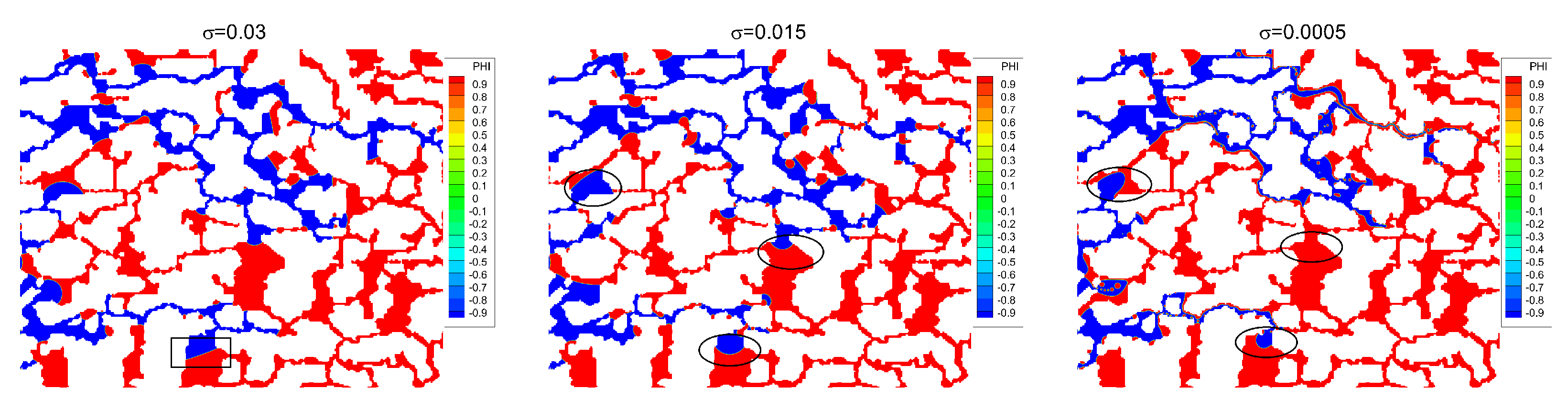
The interfacial tension between the displacing and displaced fluid is known to play an important role at the pore scale for two-phase displacement through a porous media. The same viscosity ratio ($\lambda =1$) was used and the contact angle was fixed at ${120}^{\circ }$. Figure 7 shows the fluid distributions at breakthrough for the interfacial tensions of 0.03 mu·ts${}^{-2}$, 0.015 mu·ts${}^{-2}$, and 0.0005 mu·ts${}^{-2}$. From this figure, it is seen that when the interfacial tension is as low as 0.0005 mu·ts${}^{-2}$, the viscous force prevails, the main fingers get thinner and even break up, and many fingers only occupy partial pores or throats that they pass by. Also a number of small blobs of displaced fluid are left behind at low levels of interfacial tension. When the interfacial tension increases to 0.015 mu·ts${}^{-2}$, larger blobs of the displaced fluid are trapped by the displacing fluid, and the displacing fluid flows into the large pore more easily due to higher capillary pressure, as highlighted by the black elliptical circles in Figure 7. As the interfacial tension is further increased to 0.03 mu·ts${}^{-2}$, we surprisingly found that the front of the displacing fluid can be flat inside some pores, e.g., the one surrounded by the black rectangle box in Figure 7, though most interfaces remain curved due to large capillary pressure. Meanwhile, much less of the displaced phase is left behind as the invading phase continues to move forward.

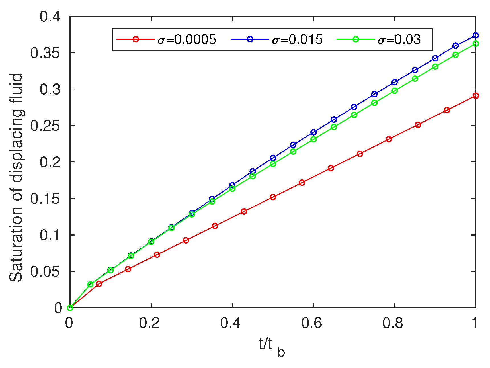
Figure 8 shows the evolution of the displacing fluid saturation for an interfacial tension of 0.0005 mu·ts${}^{-2}$, 0.015 mu·ts${}^{-2}$ and 0.03 mu·ts${}^{-2}$. It is seen that generally higher interfacial tension results in a higher saturation. The linear relationship between saturation and the evolving time is again observed.

4.4. The Contact Angle Effect

The contact angle was measured from the displaced fluid. All the contact angles were larger than ${90}^{\circ }$ in this part to simulate the imbibition process.

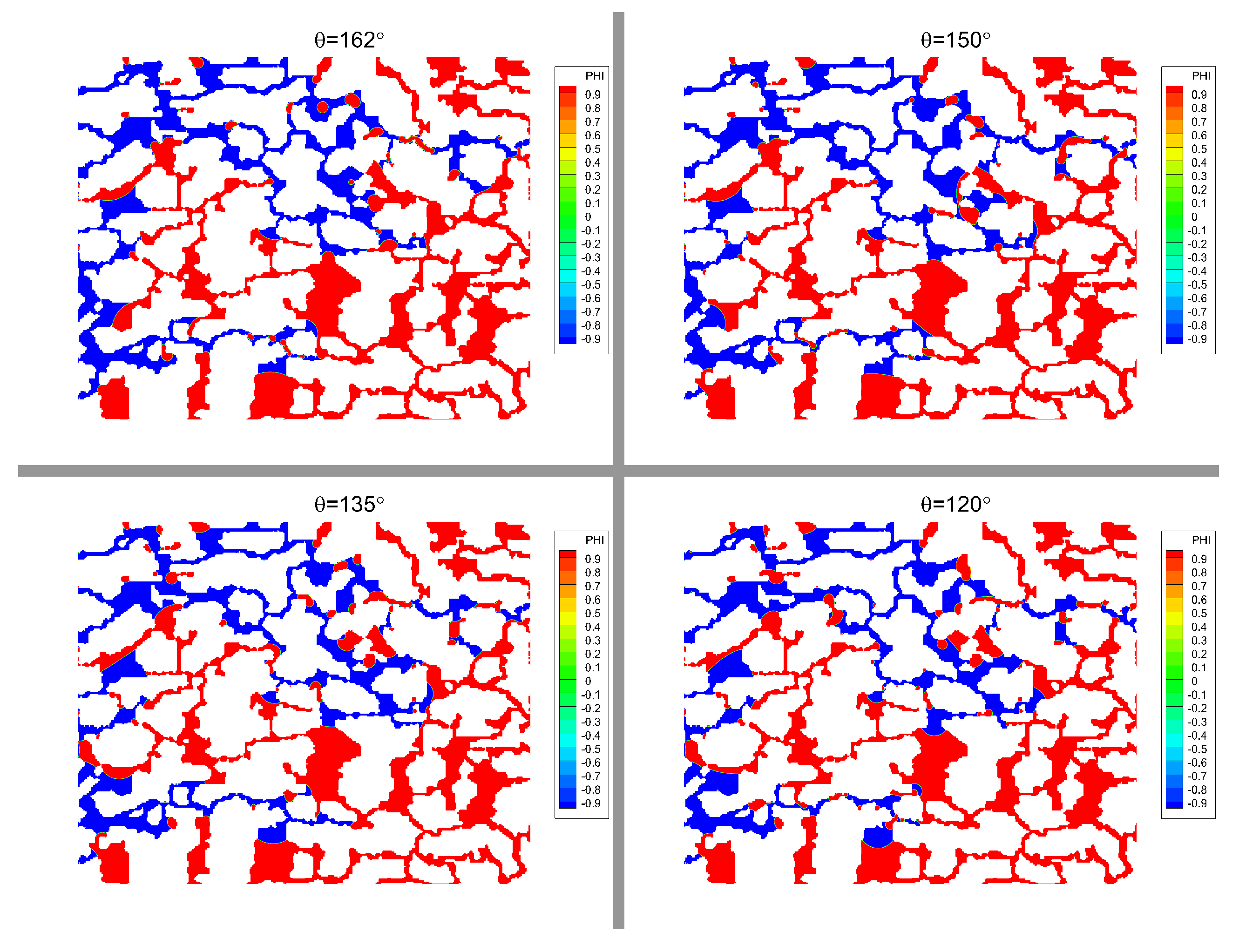
Figure 9 shows the fluid distributions when the displacing fluid breaks through at the outlet for the contact angles of ${162}^{\circ }$, ${150}^{\circ }$, ${135}^{\circ }$, and ${120}^{\circ }$. It is observed that the invading paths of the wetting fluid do not change significantly except for a few branches. An obvious difference can be seen at the contact angle of ${135}^{\circ }$ where the bottom finger advances furthermost. Figure 10 shows the evolution of the displacing fluid for different contact angles. The case of $\theta ={120}^{\circ }$ has the lowest wetting fluid saturation but its difference from the others is very small. It can also be seen from Figure 6 that the contact angle does not have a big impact on the saturation. Therefore, the contact angle has a limited effect on the efficiency of displacement in the micro-model of Berea sanstone.

5. Conclusions

The colour gradient two-phase LBM was used to study dynamic displacement of immiscible fluids in a 2D micromodel of Berea sandstone. The effects of the viscosity ratio, interfacial tension, and contact angle on the fluid distributions at breakthrough and the evolution of displacing fluid saturation were systematically investigated. When the viscosity ratio is no more than 20, a higher viscosity ratio results in a lower displacing fluid saturation which is less favourable for the recovery of the displaced fluid. However, when the viscosity ratio is larger than 20, the saturation is almost constant for both imbibition and drainage, regardless of the interfacial tension. At the viscosity ratio of unity, the displacing fluid saturation has the highest value, and it linearly increases with time.

The interfacial tension affects the flow pattern. When the interfacial tension is as low as 0.0005 mu·ts${}^{-2}$, thin viscous fingers appear. A number of small drops of displaced fluid are left behind. As the interfacial tension increases from 0.0005 mu·ts${}^{-2}$ to 0.015 mu·ts${}^{-2}$, the size of the trapped blobs increases, and the number decreases. The displacing fluid flows into large pores more easily due to the increased capillary pressure. When the interfacial tension continues to increase, smaller amount of the displaced phase is left behind as the invading phase continues to move forward. In addition, increasing interfacial tension results in a higher saturation of wetting fluid.

The contact angle generally does not change preferential flow paths except for a few branches in the imbibition, suggesting that the contact angle has limited effect on the efficiency of displacement within 2D Berea sandstone.

References

- Standnes, D.C. Scaling spontaneous imbibition of water data accounting for fluid viscosities. J. Pet. Sci. Eng. 2010, 73, 214–219. [Google Scholar] [CrossRef]
- Chang, L.C.; Tsai, J.P.; Shan, H.Y.; Chen, H.H. Experimental study on imbibition displacement mechanisms of two-phase fluid using micro mode. Environ. Earth Sci. 2009, 59, 901–911. [Google Scholar] [CrossRef]
- Chang, L.C.; Chen, H.H.; Shan, H.Y.; Tsai, J.P. Effect of connectivity and wettability on the relative permeability of NAPLs. Environ. Geol. 2009, 56, 1437–1447. [Google Scholar] [CrossRef]
- Bear, J. Dynamics of Fluids in Porous Media; Dover: Mineola, NY, USA, 1972. [Google Scholar]
- Kang, Q.; Zhang, D.; Chen, S. Immiscible displacement in a channel: Simulations of fingering in two dimensions. Adv. Water Resour. 2004, 27, 13–22. [Google Scholar] [CrossRef]
- Yiotis, A.G.; Talon, L.; Salin, D. Blob population dynamics during immiscible two-phase flows in reconstructed porous media. Phys. Rev. E 2013, 87, 033001. [Google Scholar] [CrossRef]
- Liu, H.; Valocchi, A.J.; Werth, C.; Kang, Q.; Oostrom, M. Pore-scale simulation of liquid CO2 displacement of water using a two-phase lattice boltzmann model. Adv. Water Resour. 2014, 73, 144–158. [Google Scholar] [CrossRef]
- Liu, H.; Zhang, Y.; Valocchi, A.J. Lattice Boltzmann simulation of immiscible fluid displacement in porous media: Homogeneous versus heterogeneous pore network. Phys. Fluids 2015, 27, 052103. [Google Scholar] [CrossRef] [Green Version]
- Yu, Y.; Liu, H.; Zhang, Y.; Liang, D. Color-gradient lattice boltzmann modeling of immiscible two-phase flows on partially wetting surfaces. J. Mech. Eng. Sci. 2018, 232, 416–430. [Google Scholar] [CrossRef]
- Li, Z.; Galindo-Torres, S.; Yan, G.; Scheuermann, A.; Li, L. A lattice boltzmann investigation of steady-state fluid distribution, capillary pressure and relative permeability of a porous medium: Effects of fluid and geometrical properties. Adv. Water Resour. 2018, 116, 153–166. [Google Scholar] [CrossRef]
- Ramstad, T.; Øren, P.-E.; Bakke, S. Simulation of two-phase flow in reservoir rocks using a lattice Boltzmann method. SPE J. 2010, 15, 1–11. [Google Scholar] [CrossRef]
- Andrew, G.K.; Rothman, D.H. Lattice Boltzmann model of immiscible fluids. Phys. Rev. A 1991, 43, 4320–4327. [Google Scholar]
- Rothman, D.H.; Keller, J.M. Immiscible cellular-automaton fluids. J. Stat. Phys. 1988, 52, 1119–1127. [Google Scholar] [CrossRef]
- Shan, X.; Chen, H. Lattice Boltzmann model for simulating flows with multi phases and components. Phys. Rev. E 1993, 47, 1815–1819. [Google Scholar] [CrossRef]
- Swift, M.; Orlandini, E.; Osborn, W.; Yeomans, J. Lattice Boltzmann simulations of liquid-gas and binary fluid systems. Phys. Rev. E 1996, 54, 5041–5052. [Google Scholar] [CrossRef]
- He, X.; Shan, X.; Doolen, G.D. Discrete Boltzmann equation model for nonideal gases. Phys. Rev. E 1998, 57, R13–R16. [Google Scholar] [CrossRef]
- Kalarakis, A.N.; Burganos, V.N.; Payatakes, A.C. Galilean-invariant lattice-boltzmann simulation of liquid-vapor interface dynamics. Phys. Rev. E 2002, 65, 056702. [Google Scholar] [CrossRef] [PubMed]
- Kalarakis, A.N.; Burganos, V.N.; Payatakes, A.C. Three-dimensional lattice-boltzmann model of van der waals fluids. Phys. Rev. E 2003, 67, 016702. [Google Scholar] [CrossRef] [PubMed]
- Huang, H.; Sukop, M. Multiphase Lattice Boltzmann Methods: Theory and Application; John Wiley & Sons: Hoboken, NJ, USA, 2015. [Google Scholar]
- Yang, J.; Boek, E.S. A comparison study of multi-component lattice Boltzmann models for flow in porous media applications. Comput. Math. Appl. 2013, 65, 882–890. [Google Scholar] [CrossRef]
- Chin, J.; Boek, E.S.; Coveney, P.V. Lattice Boltzmann simulation of the flow of binary immiscible fluids with different viscosities using the Shan-Chen microscopic interaction model. Philos. Trans. R. Soc. Lond. A 2002, 360, 547–558. [Google Scholar] [CrossRef] [PubMed]
- Hatiboglu, C.U.; Babadagli, T. Pore-scale studies of spontaneous imbibition into oil-saturated porous media. Phys. Rev. E 2008, 77. [Google Scholar] [CrossRef] [PubMed]
- Liu, H.; Valocchi, A.J.; Kang, Q. Three-dimensional lattice Boltzmann model for immiscible two-phase flow simulations. Phys. Rev. E 2012, 85. [Google Scholar] [CrossRef] [PubMed]
- Ba, Y.; Liu, H.; Li, Q.; Kang, Q.; Sun, J. Multiple-relaxation-time color-gradient lattice Boltzmann model for simulating two-phase flows with high density ratio. Phys. Rev. E 2016, 94, 023310. [Google Scholar] [CrossRef] [PubMed]
- Xu, Z.; Liu, H.; Valocchi, A.J. Lattice Boltzmann simulation of immiscible two-phase flow with capillary valve effect in porous media. Water Resour. Res. 2017, 53, 3770–3790. [Google Scholar] [CrossRef]
- Akai, T.; Bijeljic, B.; Blunt, M.J. Wetting boundary condition for the Lattice Boltzmann Method: Validation with analytical and experimental data. Adv. Water Resour. 2018, 116, 56–66. [Google Scholar] [CrossRef]
- Wu, R.; Kharaghani, A.; Tsotsas, E. Two-phase flow with capillary valve effect in porous media. Chem. Eng. Sci. 2016, 139, 241–248. [Google Scholar] [CrossRef]
- Ginzburg, I. Equilibrium-type and link-type lattice boltzmann models for generic advection and anisotropic-dispersion equation. Adv. Water Resour. 2005, 28, 1171–1195. [Google Scholar] [CrossRef]
- Ginzburg, I.; Verhaeghe, F.; d’Humieres, D. Two-relaxation-time lattice boltzmann scheme: About parametrization, velocity, pressure and mixed boundary conditions. Commun. Comput. Phys. 2008, 3, 427–478. [Google Scholar]
- Ginzburg, I.; Verhaeghe, F.; d’Humieres, D. Study of simple hydrodynamic solutions with the two-relaxation-times lattice boltzmann scheme. Commun. Comput. Phys. 2008, 3, 519–581. [Google Scholar]
- Timm, K.; Kusumaatmaja, H.; Kuzmin, A. The Lattice Boltzmann Method: Principles and Practice; Springer: Berlin, Germany, 2016. [Google Scholar]
- Ginzburg, I.; d’Humières, D. Multireflection boundary conditions for lattice boltzmann models. Phys. Rev. E 2003, 68, 066614. [Google Scholar] [CrossRef] [PubMed]
- Zu, Y.Q.; He, S. Phase-field-based lattice Boltzmann model for incompressible binary fluid systems with density and viscosity contrasts. Phys. Rev. E 2013, 87. [Google Scholar] [CrossRef] [PubMed]
- Brackbill, J.U.; Kothe, D.B.; Zemach, C. A continuum method for modeling surface tension. J. Comput. Phys. 1992, 100, 335–354. [Google Scholar] [CrossRef]
- Guo, Z.; Zheng, C.; Shi, B. Discrete lattice effects on the forcing term in the lattice Boltzmann method. Phys. Rev. E 2002, 65. [Google Scholar] [CrossRef] [PubMed]
- Halliday, I.; Law, R.; Care, C.M.; Hollis, A. Improved simulation of drop dynamics in a shear flow at low Reynolds and capillary number. Phys. Rev. E 2006, 73. [Google Scholar] [CrossRef] [PubMed]
- Latva-Kokko, M.; Rothman, D.H. Diffusion properties of gradient-based lattice Boltzmann models of immiscible fluids. Phys. Rev. E 2005, 71. [Google Scholar] [CrossRef] [PubMed]
- Leclaire, S.; Abahri, K.; Belarbi, R.; Bennacer, R. Modeling of static contact angles with curved boundaries using a multiphase lattice Boltzmann method with variable density and viscosity ratios. Int. J. Numer. Methods Fluids 2016, 82, 451–470. [Google Scholar] [CrossRef]
- Li, Q.; Luo, K.H.; Kang, Q.J.; Chen, Q. Contact angles in the pseudopotential lattice Boltzmann modeling of wetting. Phys. Rev. E 2014, 90. [Google Scholar] [CrossRef] [PubMed]
- Zou, Q.; He, X. On pressure and velocity boundary conditions for the lattice Boltzmann BGK model. Phys. Fluids 1997, 9, 1591. [Google Scholar] [CrossRef]
- Yiotis, A.G.; Psihogios, J.; Kainourgiakis, M.E.; Papaioannou, A.; Stubos, A.K. A lattice Boltzmann study of viscous coupling effects in immiscible two-phase flow in porous media. Colloids Surf. A 2007, 300, 35–49. [Google Scholar] [CrossRef]
- Boek, E.S.; Venturoli, M. Lattice-Boltzmann studies of fluid flow in porous media with realistic rock geometries. Comput. Math. Appl. 2010, 59, 2305–2314. [Google Scholar] [CrossRef]
- Kang, D.H.; Yun, T.S. Minimized capillary end effect during CO2 displacement in 2D micromodel by manipulating capillary pressure at the outlet boundary in lattice Boltzmann method. Water Resour. Res. 2018, 54, 895–915. [Google Scholar] [CrossRef]
- Zhang, C.; Oostrom, M.; Wietsma, T.W.; Grate, J.W.; Warner, M.G. Influence of viscous and capillary forces on immiscible fluid displacement: Pore-scale experimental study in a water-wet micromodel demonstrating viscous and capillary fingering. Energy Fuels 2011, 25, 3493–3505. [Google Scholar] [CrossRef]
- Dong, B.; Yan, Y.Y.; Li, W.Z. LBM simulation of viscous fingering phenomenon in immiscible displacement of two fluids in porous media. Transp. Porous Media 2011, 88, 293–314. [Google Scholar] [CrossRef]
Figure 1.
Relative permeabilities as a function of wetting phase saturation for two-phase concurrent flow in a 2D channel for (a) and (b) . The open circles represent the simulation results, and the solid lines are the analytical solutions from Equation (23).
Figure 2.
The 2D pore network used in the present lattice Boltzmann method (LBM) simulations. The solid grains are represented in gray, while the displacing and displaced fluids are represented in blue and red, respectively. The domain size is 1774 m by 1418 m.
Figure 3.
Porosity as a function of the domain size. L is the length of the entire micromodel, while H is its width; x refers to the distance to the left boundary, and y is the distance to the bottom boundary. For each point shown above, the same scaling was applied to x and y, i.e., x/L = y/H.
Figure 4.
Fluid distributions at breakthrough for a wetting fluid invading a porous medium initially saturated with a non-wetting fluid. The wetting fluid (indicated in blue) is injected from the left side, and the viscosity ratio equals 1, 2, 5, and 10, respectively.
Figure 5.
Evolution of the displacing fluid saturation for the viscosity ratio increased from 1 to 30 at mu·ts and (imbibition). Note that the time is normalized by , defined as the time at which the breakthrough occurs.
Figure 6.
Displacing fluid saturation as a function of viscosity ratio for the four typical cases listed in Table 1.
Figure 7.
Fluid distributions at breakthrough for a wetting fluid invading a porous medium initially saturated with a non-wetting fluid. The wetting fluid (indicated in blue) is injected from the left side and the values of the interfacial tension are 0.03 mu·ts, 0.015 mu·ts, and 0.0005 mu·ts from the left to right.
Figure 8.
Evolution of the displacing fluid saturation for the interfacial tension of 0.0005 mu·ts, 0.015 mu·ts and 0.03 mu·ts.
Figure 9.
Fluid distributions at breakthrough for a wetting fluid invading a porous medium initially saturated with a non-wetting fluid. The wetting fluid (indicated in blue) is injected from the left side and the values of the contact angle are , , , and , respectively.
Figure 10.
Evolution of the displacing fluid saturation for contact angles of , , , and .