Scale Analysis of Wavelet Regularization Inversion and Its Improved Algorithm for Dynamic Light Scattering

Abstract

In the large inversion range, the wavelet-regularization inversion method (WRIM) is an effective method for improving the inversion accuracy of dynamic light scattering (DLS) data. However, the initial decomposition scale (IDS) of this method has a great effect on the inversion accuracy. The particle size distribution (PSD) obtained from inappropriate IDS is not optimal. We analyze the effect of the different IDS on the inversion result in this paper. The results show that IDS of the smallest relative error should be chosen as the optimal IDS. However, because the true PSD is unknown in the practical measurements, this optimal IDS criterion is infeasible. Therefore, we propose an application criterion determining the optimal IDS. Based on this criterion, an improved WRIM with the optimal IDS is established. By the improved WRIM, high accuracy inversion PSD is obtained from DLS data. The simulated and experimental data demonstrate the effectiveness of this algorithm. Besides, we also further study the effect of the data noise on the optimal IDS. These studies indicate that the optimal IDS usually shows a downward trend with an increase of noise level.

1. Introduction

DLS is a widely used technique for measuring the PSD of ultrafine particles in suspension [1,2,3,4]. The principle of DLS is based on the Brownian motion of particles in suspension, which leads to the fluctuation of scattered light. This fluctuation contains particle size information. DLS technology obtains PSD by measuring the autocorrelation function (ACF) of scattered light intensity [5,6]. Retrieving the PSD information from ACF (measurements data) is known as a highly ill-posed problem. The small disturbances in the measurement data may lead to serious deviation in PSD. In order to deal with this problem, the numerous inversion approaches have been proposed to estimate the PSD from DLS data, such as the cumulants method [7,8], constrained regularization method (CONTIN) [9,10], Laplace transform method [11], the nonnegative leastsquares method (NNLS) [12], maximum likelihood method [13], exponential sampling method [14], nonnegative TSVD method [15], Bayesian inversion method [16,17,18], the maximum entropy method [19], and the various intelligences methods [20,21,22,23,24,25]. In addition, various improved algorithms have constantly emerged [26,27,28,29]. Each of these algorithms has its own advantages and limitations. In general, these approaches solve the problem in a single-scale space and a fixed inversion range. The inversion range has been fixed during the solution. In fact, the inversion range is related to the inversion accuracy of PSD. The appropriate inversion range is the precondition for the various inversion methods mentioned above to obtain a good PSD. The inappropriate inversion range is likely to get lower accuracy or even wrong inversion results. In practice, the inversion range can be manually adjusted based on the repeated inversions. However, in many cases, the manual method is not feasible, for example, polymeric materials study and biological analysis [30,31]. The former inversion results have been no longer applicable for the latter inversion. Thus, the inversion approach with fixed inversion range is difficult to give the accurate inversion PSD.

WRIM is an effective method for obtaining the optimal PSD in preselecting a large inversion range. The method gradually approaches the true particle size range by adaptive adjustment of the inversion range and has high inversion accuracy [32]. In WRIM, maximum scale of wavelet decomposition is called as initial decomposition scale (IDS). For convenience of expression, IDS N indicates that the initial decomposition scale is N. WRIM only uses IDS 4 in Reference [32]. However, in the application, IDS has great effect on the inversion accuracy. PSD obtained from unsuitable IDS is not optimal. Sometimes, the recovery PSD is even worse than the recovery PSD of the traditional single-scale method. Therefore, the scale effect of WRIM is carried on further studies in this paper. Besides, considering the application, an improved WRIM with the optimal IDS is proposed in this paper. By the improved algorithm, the high-accuracy inversion PSD is obtained from DLS data. Finally, the effectiveness of the algorithm is demonstrated by the simulated and experimental data. This study has a very important role for improving the measurement accuracy of DLS data.

2. Principle of WRIM for DLS

2.1. Regularization Inversion of DLS

In DLS, PSD can be inverted from the normalized electric field ACF.

$$g\left(\mathsf{\tau }\right)={\displaystyle {\int }_0^{\infty }G(\Gamma )\exp (-\Gamma \mathsf{\tau })}d\Gamma$$

(1)

in which $\Gamma$ is the decay linewidth, $\mathsf{\tau }$ is the delay time, and $G(\Gamma )$ is the normalized distribution function of the decay linewidth. $G(\Gamma )$ contains the PSD information and satisfies the conditions ${\displaystyle {\int }_0^{\infty }G(\Gamma )}d\Gamma =1$. According to the following three formulas, PSD can be solved form the ill-posed Equation (1).

$$\{\begin{array}{l}\Gamma =D{q}^2\\ q=\frac{4\pi l}{\lambda }\sin \left(\frac{\theta }{2}\right)\\ D=\frac{k_{\mathrm{B}}T}{3\pi \eta d}\end{array}$$

(2)

in which $q$ is the scattered vector, $D$ is diffusion coefficient, $\lambda$ is the wavelength of the incident light in vacuum, $\theta$ is scattering angle, l is the refractive index of the solvent, T is the absolute temperature, $k_{\mathrm{B}}$ is the Boltzmann constant, d is the particle diameter, and $\eta$ is the solvent viscosity.

To solve PSD, Equation (1) can be discretized as

$$g\left({\mathsf{\tau }}_j\right)={\displaystyle \sum _{i=1}^{N}G\left({\Gamma }_i\right)}\exp (-{\Gamma }_i{\mathsf{\tau }}_j)$$

(3)

in which j is the channel number of ACF and i is the grading number of the inversion particles. Equation (3) can be replaced as following matrix equation

$$Ax=b$$

(4)

in which elements of A, $x$, and b are $a_{i,j}=\exp (-{\Gamma }_i{\mathsf{\tau }}_j)$, $x_i=G({\Gamma }_i)$, and $b_j=g({\mathsf{\tau }}_j)$, respectively. $i$ is the sampling point spaced at the particle size steps along the PSD range [dmin, dmax], and $j$ is the channel number of the correlator. Theoretically, PSD can be obtained by directly solving Equation (4). However, because of the ill-posed nature of Equation (4), its accurate solution cannot be obtained in the practical application. We usually solve its approximate solution using the various optimization algorithms. The optimization solution of Equation (4) can be expressed as the following least square (LS) problem [33]:

$${\Vert Ax-b\Vert }_2^2=\min =x_{LS}$$

(5)

In Equation (5), if ACF contains the noises, the solution $x$ has a large deviation and even instability. The traditional Tikhonov regularization method is an effective way for this kind problem [34,35]. The solution of Equation 4 can be written as [36]:

$$M^{\alpha }[x,b]={\Vert Ax-b\Vert }_2^2+\alpha {\Vert x\Vert }_2^2$$

(6)

in which $\alpha$ is regularization parameter. The regularization solution of Equation (6) is as follows:

$$x=\min \{M^{\alpha }[x,b]\}$$

(7)

In this paper, the regularization parameter is defined by L-curve criterion [37,38].

2.2. Inversion Principle of WRIM

Owing to the inevitable noise of ACF and the inappropriate inversion range, it is extremely easy for the traditional single-scale optimization of Equation (7) to fall into local minimum value. Therefore, we obtained the optimal solution with much difficulty. Wavelet transform is a new multi-scales analysis method that can provide a “time-frequency” window with frequency change [39,40]. It is an ideal tool for time-frequency analysis and signal processing. It gradually decomposes the signal on the multi-scales through the expansion and translation operation, and finally meets the requirements of adaptive analysis of signal. Therefore, the wavelet transform is widely used in many fields such as industry, medicine, and military. Considering the multi-scales characteristics of the wavelet transform, the wavelet inversion strategy that can accelerate the convergence, enhance the stability, and overcome the disturbance of local minima is developed [41,42]. Using this inversion strategy, the global optimal solution can be quickly searched out. Taking the wavelet transform of IDS 4 shown in Figure 1 as an example, we introduce its specific principle. In Figure 1, scale 1 to scale 4 corresponds to the scale from fine to coarse. The original ACF A₁ is decomposed into coarse and fine two sub-spaces. The signal parts corresponding to the fine and coarse sub-spaces are A₂, D₂, respectively. A₂ corresponds to the approximation part, namely, overall trend of ACF. D₂ corresponds to the detail part, namely, removed noise form original ACF. Then, the approximation part A₂ continues to be decomposed into A₃ and D₃. Thus, the detail part is gradually removed from ACF. This process continues repeatedly until the decomposition scale reaches the coarsest scale. With the increase of decomposition scale, ACF noise of the coarser space is gradually removed, and then ACF of this space becomes relatively smoother. In Figure 1, ACF can be written as

ACF(A₁) = A₂ + D₂ = A₃ + D₃ + D₂ = A₄ + D₄ + D₃ + D₂

(8)

Through the multi-scale decomposition, the original ACF is composed into the approximation parts A₂, A₃, and A₄ in the different sub-spaces. Correspondingly, the original inversion problem is divided into many sub-problems.

$$A_i{x}_i=b,i=1,2,3,4$$

(9)

in which $A_i,x_i$ is similar to the matrix $A$ and $x$ in Equation (4). They are calculated in the diameter inversion range [dmin, dmax] of the different sub-spaces.

Because A₄ has the best smoothness in the coarsest space, even within larger initial inversion range, the optimal value of this sub-problem is easy to solve. According to this global optimal value, we can get the approximate inversion range close to true value. Then, the scale becomes finer again, and the detailed part D₄ of ACF is gradually retrieved. The sub-problem corresponding to A₃ is inverted above near true inversion range. Therefore, the global optimal value of this scale can be easily found. Repeatedly, as the decomposition scales become finer, the inversion range gradually becomes closer to the true value. When the scale reaches 1, the final optimal PSD is obtained in the inversion range closest to the true values. The flow chart of this method is shown in Figure 2.

In Figure 2, $V_i$, $i=1,2\cdots J$ denote different sub-spaces, and $J$ is IDS. $I_{J-1}^J$ represents the wavelet decomposition from $V_{J-1}\to V_J$; $I_J^{J-1}$ represents the wavelet reconstruction from $V_J\to V_{J-1}$; $R_J$ expresses the inversion operation in the Jth sub-space; $[d_{\min J},d_{\max J}]$ represents the PSD range retrieved in the Jth sub-space, which is used as the initial inversion range on the J − 1th scale. If IDS 1 is used in WRIM, it means that the traditional Tikhonov regularization method is employed.

In Figure 2, the wavelet transform is achieved by Mallat algorithm [43,44]. Its decomposition and reconstruction formulas are expressed as

$$\{\begin{array}{l}{a}_{j+1}(k)={\displaystyle \sum _{m=-\infty }^{\infty }{a}_j}(m)h_0(m-2k)\\ d_{j+1}(k)={\displaystyle \sum _{m=-\infty }^{\infty }{a}_j}(m)h_1(m-2k)\end{array}$$

(10)

$$a_j(k)={\displaystyle \sum _{m=-\infty }^{\infty }{a}_{j+1}(k)}{h}_0(k-2m)+{\displaystyle \sum _{m=-\infty }^{\infty }{d}_{j+1}(k)}{h}_1(k-2m)$$

(11)

in which $h_0(k)$ and $h_1(k)$ are the conjugate filter coefficients defined in wavelet analysis, respectively. They are related to the wavelet bases. $a_j(k)$ and $d_j(k)$ are approximation coefficient and the detail coefficient of the wavelet decomposition, respectively. Here, j is the decomposition scale number, m is the time series shift index, and k is the wavelet coefficient sequence index.

In the different subspaces, the different sub-problems are still sub-inversion problems with different degrees of ill-posedness. For the inversion of each sub-problem, the traditional Tikhonov regularization method is used. Considering non-negative characteristic of PSD, the negative inversion PSD should be set to zeros. In the process of solving WRIM, the inversion error of the sub-problem is so large in the coarse scale space that the inversion range determination of its near fine-scale space will be affected. Therefore, 3 to 5 points of the marginal PSD are usually set to zeros in the coarse scale space.

3. Analysis of Scale Effect of Simulation Data

3.1. Simulation Experiment Parameters and Conditions

In WRIM, in order to study the effect of IDS on the inversion results, ACF data of the different PSDs are simulated. The PSD is described by Johnson’s SB function [45].

$$f(x)=\frac{\sigma }{\sqrt{2\pi }\left(x_{\max }-x_{\min }\right)}{\left[t(1-t)\right]}^{-1}\exp \left\{-0.5{\left[u+\sigma \ln \left(\frac{t}{1-t}\right)\right]}^2\right\}$$

(12)

in which $t=\left(x-x_{\min }\right)/\left(x_{\max }-x_{\min }\right)$ is the normalized particle size, $x_{\min }$ and $x_{\max }$ are the maximum and minimum particle diameter, respectively. For the simulation, the following experimental parameters were used: $\lambda =632.8$ nm, $\theta$ = 90°, l = 1.331, T = 298 K, $k_{\mathrm{B}}$ = 1.3807 × 10⁻²³ J·K⁻¹, and $\eta$ = 0.89 × 10⁻³ mPa.s. To compare the inversion results of the different IDSs, the relative error (RE) of PSD is introduced as a measure index in the different IDSs. It is expressed as

$$RE={\Vert x-x^{\prime }\Vert }_2/{\Vert x^{\prime }\Vert }_2\times 100\%$$

(13)

in which $x$, $x^{\prime }$ are the inversion PSD and the true PSD, respectively.

In addition, in the following simulation study, due to the inversion range adjustments of WRIM, the particle size steps of the inversion PSDs are different on the different IDSs. Therefore, the inversion PSDs of the different IDSs cannot be directly compared. To compare the inversion results of the different IDSs, the inversion PSD is uniformly converted to the standard of simulation particle size step in the following Figures 3–6 and 8.

3.2. Inversion Analysis on Different IDSs

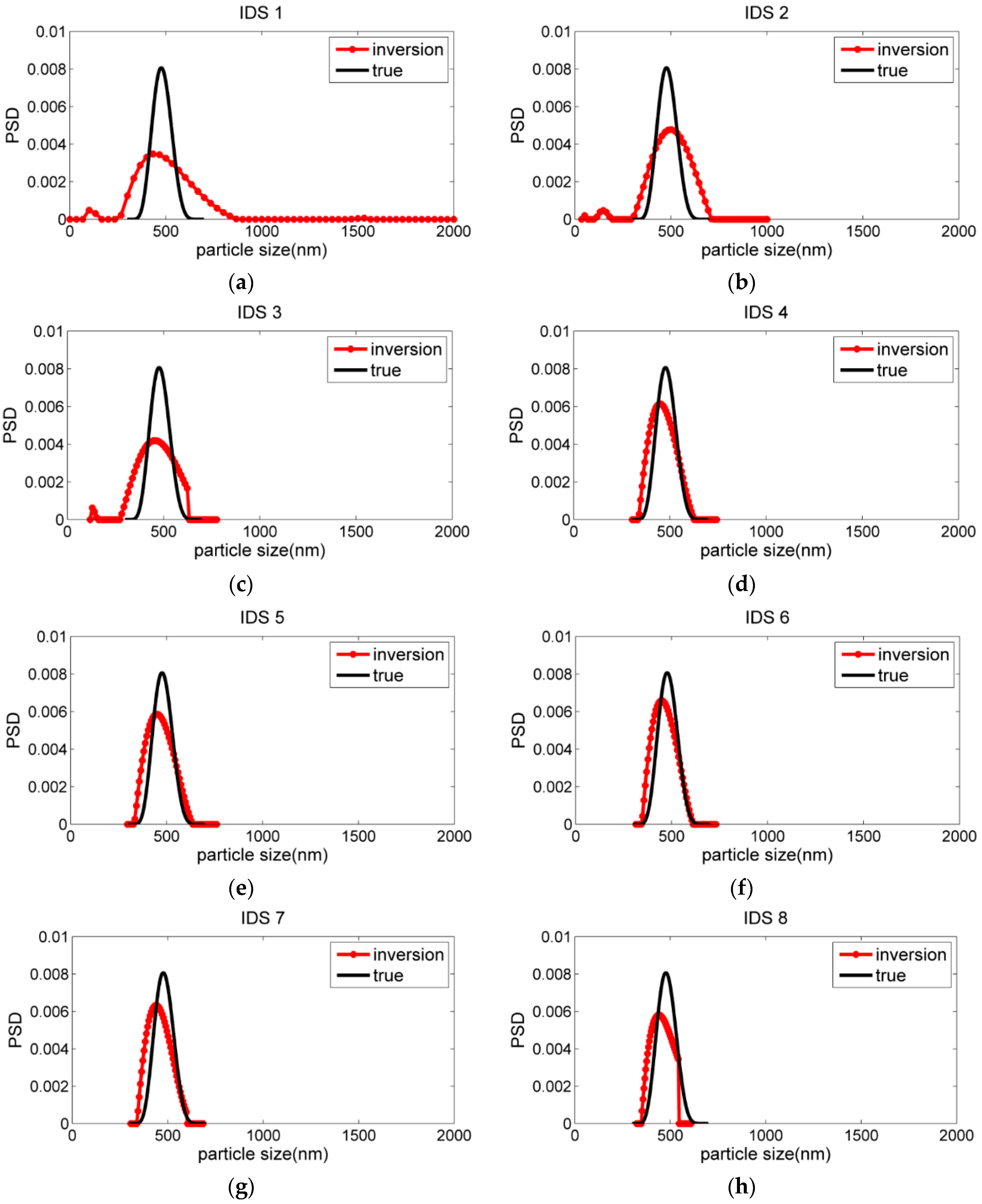
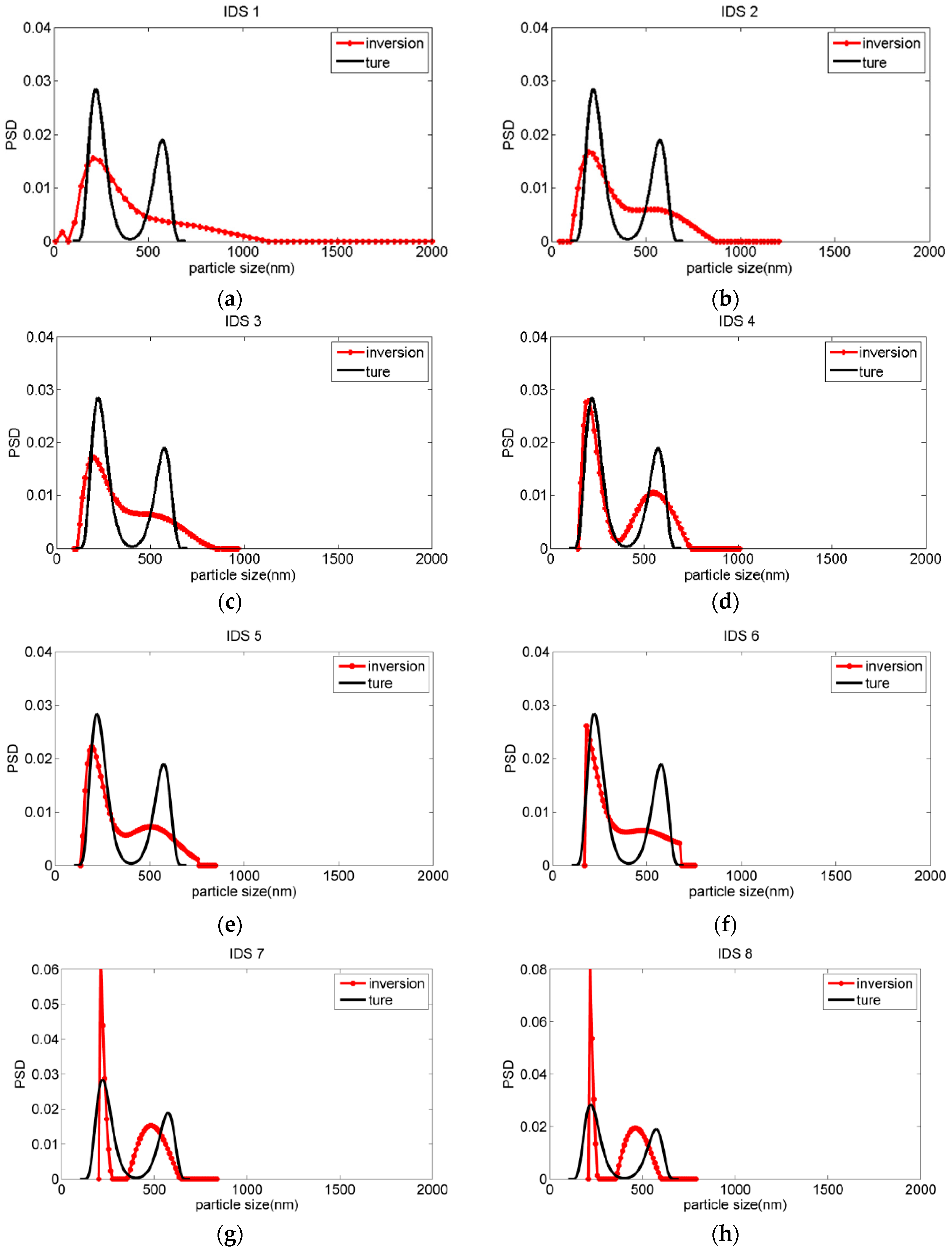
On the different IDSs, 300 nm~700 nm unimodal PSD (true peak: 477.01 nm) and 100 nm~700 nm bimodal PSD (true peak: 220.01 nm, 575.01 nm) were taken for analysis. The unimodal PSD shares the parameters $u$ = 0.4, $\sigma$ = 2.0. The bimodal PSD shares the parameters $u_1$ = −3, ${\sigma }_1$ = 2.4; $u_2$ = 3, ${\sigma }_2$ = 2.4. On 8 different IDSs, ACFs with the standard uniform distribution of noise level 0.001 are inverted by WRIM. In the inversion, the initial inversion range and wavelets base are [1, 2000] and “db25”, respectively. The inversion results are shown in Figure 3 and Figure 4 and

Table 1. Inversion data of the unimodal and bimodal distribution particles on the different IDSs.

IDS	Unimodal Distribution Particles		Bimodal Distribution Particles
	Peak Value (nm)	RE	Peak Value (nm)	RE
1	434.11	0.6129	—, —	0.6174
2	501.30	0.5261	197.94, 526.84	0.5485
3	458.40	0.5207	196.72, 459.41	0.5511
4	449.96	0.3471	205.79, 579.47	0.3334
5	451.36	0.3598	193.96, 502.70	0.4668
6	452.81	0.3257	188.89, 479.82	0.4998
7	439.28	0.3963	222.10, 487.17	0.8255
8	437.74	0.4051	217.95, 460.08	1.1538

.

Figure 3 and Figure 4 and Table 1 show that, with the change of IDS, RE is also changed. For the bimodal particles, WRIM cannot distinguish between the two peaks on IDS 1, and the bimodal characteristics of the inversion PSD are not obvious on IDS 2, 3, 5, and 6. On the contrary, the bimodal characteristics of IDS 4, 7, and 8 are obvious. However, the PSDs of IDS 7 and 8 have large errors, 0.8255 and 1.1538, respectively, and have also lost part of the information. The cause of this phenomenon can be explained as follows: When IDSs are 7 and 8, the inversion range of scale 1 is adjusted so it is so small that it is less than the true PSD range in WRIM. Overall, RE of IDS 4 is minimum. The inversion PSD and peak value of the IDS are the closest to true value. For the unimodal particles, the peaks recovered from IDS 1 to 3 are wide and have burrs. In contrast to IDS 1 to 3, PSDs inverted from IDS 4 to 7 are the smooth single peak and coincide with the true PSD. Due to small inversion range of scale 1, the part inversion PSD is also lost on IDS 8. Considering $\min \left[RE\right]$, the inversion PSD of IDS 6 is best. Therefore, through the above analysis, the choice of IDS has a great impact on the accuracy of the recovery PSD in WRIM. We should select the optimal IDS. The following research finds that the optimal IDS is related to noise level of ACF.

3.3. Effect of ACF Noise on Optimal IDS

The noise level of ACF will be around 0.001, or even lower in the DLS measurement [46], so simulated experiments were performed at noise level of 0.0001, 0.005 and 0.001, respectively. Therefore, the simulated experiments were performed at noise level of 0.0001, 0.005, and 0.001, respectively. A large number of the simulation experiments show that, when IDS is bigger than 7 in WRIM, the inversion PSDs of the particles will be distorted. Thus, in the following experiments, we chose IDS 7 as the maximum. At three kinds of the noise levels, 0.0001, 0.005 and 0.001, respectively, the noisy ACFs of above two kinds of PSDs were inverted by WRIM. IDSs are used from 1 to 7 in the inversion. The inversion results are shown in Figure 5. Comparing RE on various IDSs, the PSD recovered at the minimum RE is optimal, and the corresponding scale is the optimal IDS. The inversion data of two kinds of PSDs are shown in

Table 2. Inversion data of the unimodal and bimodal particles under the different noise levels.

Noise Level	Unimodal Particles			Bimodal Particles
	Peak Value (nm)	RE	Optimal IDS	Peak Value (nm)	RE	Optimal IDS
0.0001	477.22	0.1037	7	233.35, 551.45	0.2411	5
0.0005	457.98	0.2711	6	208.26, 562.04	0.3402	4
0.001	454.81	0.3118	6	205.79, 550.72	0.3725	4

.

From Figure 5, we can find that, with the increase of the noise level, the optimal IDS shows a downward trend. When the noise level is 0.0001, the optimal IDS of 300 nm~700 nm particles is 7. However, when the noise levels add to 0.0005 and 0.001, respectively, their optimal IDSs are reduced to 6 and 6. For 100 nm~700 nm particles, the noise levels are gradually added to 0.0001, 0.0005, and 0.001, respectively. Their corresponding optimal IDSs also show a downward trend, composed of 5, 4, and 4, respectively.

The reason for above phenomenon can be interpreted from the following inversions of 100 nm~700 nm bimodal particles. In the inversion ranges of [120 nm, 1000 nm] and [100 nm, 700 nm], respectively, we inverted for ACFs with the noise level of 0.0001 and 0.001 in the space of scale 1. The inversion results are shown in Figure 6. From the results, we can see, at the low noise level 0.0001, when the inversion range is close to the true range of [100 nm, 700 nm], the inversion result is closer to the true PSD. On the contrary, when the inversion range is increased to [120 nm, 1000 nm], the error of its inversion PSD also increases. However, at the greater noise level 0.001, it is difficult to get the correct inversion result in the true inversion range of [100 nm, 700 nm]. Conversely, the result with greater inversion range [120 nm, 1000 nm] is more accurate. From the above inversion, we can draw a conclusion that the inversion of the greater noise data demands the greater inversion range. When IDS is large, it means that the inversion range of scale 1 becomes too small after multiple sub-inversions. Generally speaking, it is difficult to get the correct inversion result in the case of high noise. Therefore, ACF contains the higher noise level, so IDS should be smaller. In other words, the optimal scale of WRIM usually shows a downward trend with the increase of data noise.

4. Improved WRIM with Optimal IDS

Because the true PSD is unknown, the criterion of minimum RE is usually difficult to use to determine the optimal IDS in practice. Considering the application, there should be a feasible criterion for determining the optimal IDS. According to the principle of WRIM, the inversion accuracy of PSD is ultimately determined by the sub-problem on the scale 1.

$$A_1{x}_1=b$$

(14)

Because the inversion of PSD is actually a fitting problem of the measurement ACF curve, the residual norm ${\Vert A_1{x}_1-b\Vert }_2^2$ is used to describe fitting error between the measuring ACF and the fitting ACF. On the condition of non-noise and calculation error in Equation (14), the solution $x_1$ with $\min {\Vert A_1{x}_1-b\Vert }_2^2$ can be as the recovered PSD, but the restrictions are not satisfied in the practical measurements. Actually, the solution is often rough and unstable. In order to ensure the smoothness and stability of the solution, the solution norm ${\Vert x_1\Vert }_2^2$ is also considered. Under $\min {\Vert x_1\Vert }_2^2$ condition, solution $x_1$ has good smoothness and stability. In order to consider the accuracy and smoothness, the regularization parameter ${\alpha }_1$ of Equation (14) is usually used to adjust the balance between $\min {\Vert A_1{x}_1-b\Vert }_2^2$ and $\min {\Vert x_1\Vert }_2^2$. Thus, for the sub-problem on the scale 1, minimization of the sum of its ACF residual norm and the regularization solution norm can be used for checking the inverting accuracy of the PSD under the different IDS. In other words, following equation can be taken as the criterion of the optimal IDS.

$$\min \left[{\Vert A_1{x}_1-b\Vert }_2^2+{\alpha }_1{\Vert x_1\Vert }_2^2\right]$$

(15)

Equation (15) is exactly the Tikhonov regularization problem of Equation (14).

In the practical application, in order to considering the above criterion, we improve the original WRIM algorithm. The improved WRIM sets IDS from 1 to maximum N. In general, maximum N may be set to 7. On each IDS i, the improved WRIM invert ACF data and calculates the value $EX(i)={\Vert A_1^{}{x}_1-b\Vert }_2^2+{\alpha }_1{\Vert x_1\Vert }_2^2$. Comparing $EX(i)$, $i$ with $\min \left[EX(i)\right]$ is the practical optimal IDS. Its inversion PSD is the inversion result of the improved WRIM. Therefore, we can see that the improved WRIM obtains the practical optimal IDS through the minimization of sub Tikhonov regularization problem on scale 1. The flow chart of this algorithm is shown in Figure 7.

In order to prove the validity of the improved WRIM, in the different initial inversion ranges, the simulated data of the noise level 0.001 are inverted by this algorithm. The ACFs originate from following four kinds of simulated particles: 10 nm~150 nm, 100 nm~600 nm, 90 nm~800 nm, and 50 nm~500 nm. Moreover, in order to explain the rationality of the improved WRIM, we also inverted these simulation data by WRIM with $\min \left[RE\right]$. For convenience of the following statements, we call it as WRIM-RE. Actually, IDSs determined by WRIM-RE is true optimal IDS, and IDSs determined by improved WRIM is practice optimal IDS. The inversion PSDs recovered by two kinds of criterions are shown in Figure 8. Their corresponding data are shown in

Table 3. Inversion data of the optimal IDS determined by the improved WRIM and WRIM-RE.

Particles	Inversion Range	WRIM-RE		Improved WRIM
		True Optimal IDS	RE	Practice Optimal IDS	RE
10 nm~150 nm	[1, 600]	3	0.0672	3	0.0672
100 nm~600 nm	[1, 2000]	5	0.1325	5	0.1325
90 nm~800 nm	[1, 2000]	3	0.3181	3	0.3181
50 nm~500 nm	[1, 1500]	3	0.3879	5	0.4015

. Besides, in order to compare the inversion results of the improved algorithm and traditional Tikhonov regularization method (namely IDS 1), the inversion PSDs of IDS 1 are also given in Figure 8.

Table 3 and Figure 8 show that, for 10 nm~150 nm, 100 nm~600 nm, and 90 nm~800 nm particle systems, PSDs of the practice optimal IDSs coincide with PSDs of the true optimal IDSs. Their corresponding optimal IDSs are 3, 5, and 3, respectively. Compared with the traditional single-scale method, the inversion results of the optimal IDS are significantly closer to the true PSD. A large number of the experiments show that the practice optimal IDS is mostly consistent with the true optimal IDS. However, in a few cases, there are inconsistencies. The inversion results can be seen from Table 3. For 50 nm~500 nm particle system, the practice optimal IDS 5 is inconsistent with the true optimal IDS 3. However, the difference between the two REs is relatively small—only 0.0136. Moreover, the inversion PSD of improved WRIM is also obviously better than that of IDS 1. Overall, improved WRIM can be used for DLS inversion.

5. Inversion Analysis of Experimental Data

The experimental data of 300 nm unimodal particles and 100 nm/450 nm bimodal particles were obtained from Brookhaven instruments. The experiment system is shown in Figure 9, which mainly involves vertically polarized He-Ne laser, sample pool, detector, and correlator. In the experiment, the temperature is 298.15 K wavelength is 632.8 nm, the scattered angle is 90°, and the dispersion medium is the pure water, respectively. In the inversion range [1, 1200] and [1, 1500], the experimental data of unimodal particles and bimodal particles were inverted by the original WRIM from IDS 1 to 7, respectively. In order to compare the inversion results of the different IDSs, the inversion PSD of the different IDSs are uniformly converted to particle size step standard of IDS 7. The inversion results are shown in Figure 10. From Figure 10, the inversions PSDs of 300 nm unimodal particles have many sub-peaks on IDS 1, 2, and 3. The recovered PSDs of other IDSs are single peak. The corresponding ${\Vert A_1{x}_1-b\Vert }_2^2+{\alpha }_1{\Vert x_1\Vert }_2^2$ of IDS 3 is minimum 0.2541. For 100 nm/450 nm bimodal particles, the inversion PSDs of IDS 1 are not obvious double peaks and have small sub-peaks. The results of IDS 7 are obviously distorted. Conversely, the results of other scales are double peaks. The corresponding ${\Vert A_1{x}_1-b\Vert }_2^2+{\alpha }_1{\Vert x_1\Vert }_2^2$ of IDS 6 has minimum of 0.1223. Therefore, for above two kinds of particles, the practice optimal IDSs are 3 and 6, respectively. The inversion PSDs of the improved WRIM are the results of IDS 3 and 6.

Moreover, to verify the inversion effect of the improved WRIM, above experimental data also was retrieved by CONTIN method widely used by various instruments. Figure 11 is the comparison of the PSDs recovered by the improved WRIM, CONTIN, and the traditional regularization method (IDS 1). In order to compare the three methods, the inversion results of other two methods are unified as the standard of CONTIN in the Brookhaven instrument. From Figure 11 and

Table 4. Inversion data of three methods.

Method	300 nm Unimodal Particles		100 nm/450 nm Bimodal Particles
	Peak Value (nm)	Peak Value Error %	Peak Value (nm)	Peak Value Error %
IDS 1	—	—	—	—
CONTIN	316.23	5.41	94.06,376.27	5.94, 16.38
Improved WRIM	385.56	4.81	109.06, 455.52	9.06, 1.23

, for the unimodal and bimodal particles, the results of the improved WRIM are the standard single peak and double peaks. Their peak value errors are 4.81% and 9.06%/1.23%. Compared with the CONTIN method, although the first peak value error of bimodal particles increases by 3.12%, the second peak value error decreases by 15.15%. Therefore, in general, we can believe that the inversion PSDs of the improved WRIM are much better than the CONTIN method. Compared with the traditional method, the improved WRIM has a more obvious advantage. Thus, the experimental data also confirm the conclusion of the simulation data.

6. Conclusions

When WRIM is used to invert DLS data, IDS of WRIM has a great effect on the inversion accuracy. If the choice of IDS is inappropriate, the inversion results of WRIM may not be optimal. In order to guide the use of WRIM, the scale effect of WRIM is carried on further studies in this paper. Through the studies, the following conclusions are drawn: (1) The relative errors of the inversion PSD and the true PSD vary on the different IDSs. In order to improve the inversion accuracy of PSD, the IDS with minimum relative error should be chosen as the optimal IDS. (2) In WRIM, the optimal IDS is related to the noise level of DLS data. When uniformly distributed noises are added, in the same inversion range, the optimal IDS usually shows a downward trend with the increase of noise level. Most importantly, considering the practical measurement, the true PSD is unknown. Minimum relative error as the criterion determining optimal IDS is infeasible. A practical application criterion determining the optimal IDS is put forward. This criterion obtains the optimal IDS through the minimization of the sub Tikhonov regularization problem on scale 1. According to this criterion, an improved WRIM is proposed in this paper. By means of the improved algorithm, high accuracy inversion PSD is obtained from DLS data.

References

- Li, L.; Yang, K.C.; Li, W.; Wang, W.Y.; Guo, W.P. A recursive regularization algorithm for estimating the particle size distribution from multiangle dynamic light scattering measurements. J. Quant. Spectrosc. Radiat. Transf. 2016, 178, 244–254. [Google Scholar] [CrossRef]
- Zhu, X.; Shen, J.; Song, L. Accurate Retrieval of Bimodal Particle Size Distribution in Dynamic Light Scattering. IEEE Photonics Technol. Lett. 2015, 28, 311–314. [Google Scholar] [CrossRef]
- Robert, F. Particle Sizing in the Submicron Range by Dynamic Light Scattering. KONA Powder Part. 1993, 11, 17–32. [Google Scholar] [CrossRef] [Green Version]
- Takahashi, K.; Kato, H.; Saito, T. Precise measurement of the size of nanoparticles by dynamic light scattering with Uncertainty Analysis. Part. Part. Syst. Charact. 2008, 25, 31–38. [Google Scholar] [CrossRef]
- Li, Z.M.; Shen, J.; Sun, X.M.; Wang, Y.J. Nanoparticle Size Measurement from Dynamic Light Scattering Data Based on Autoregressive Model. Laser Phys. Lett. 2013, 10, 095701–095705. [Google Scholar] [CrossRef]
- Liu, W.; Sun, X.M.; Shen, J. A V-curve criterion for the parameter optimization of the Tikhonov regularization inversion algorithm for particle sizing. Opt. Laser Technol. 2012, 44, 1–5. [Google Scholar] [CrossRef]
- Koppel, D.E. Analysis of macromolecular polydispersity in intensity correlation spectroscopy: The Method of Cumulants. J. Chem. Phys. 1972, 57, 4814–4820. [Google Scholar] [CrossRef]
- Frisken, B.J. Revisiting the method of cumulants for analysis of dynamic light scattering data. Appl. Opt. 2001, 40, 4087–4091. [Google Scholar] [CrossRef] [PubMed]
- Provencher, S.W. CONTIN: A general purpose constrained regularization program for inverting noisy linear algebraic and integral equations. Comput. Phys. Commun. 1982, 27, 229–242. [Google Scholar] [CrossRef]
- Provencher, S.W. A constrained regularization method for inverting data represented by linear algebraic or integral equations. Comput. Phys. Commun. 1982, 27, 213–227. [Google Scholar] [CrossRef]
- McWhirter, J.G.; Pike, E.R. On the numerical inversion of the Laplace transform and similar Fredholm integral equations of the first kind. J. Phys. A Math. Theor. 1978, 11, 1729–1745. [Google Scholar] [CrossRef]
- Varah, J.M. On the Numerical Solution of Ill-Conditioned linear systems with applications to Ill-Posed problems. Siam J. Numer. Anal. 1973, 10, 257–267. [Google Scholar] [CrossRef]
- Sun, Y.F.; Walker, J.G. Maximum likelihood data inversion for photon correlation spectroscopy. Meas. Sci Technol. 2008, 19, 115302. [Google Scholar] [CrossRef]
- Ostrowsky, N.; Sornette, D.; Parker, P.; Pike, E.R. Exponential sampling method for light scattering polydispersity analysis. J. Mod Opt. 1981, 28, 1059–1070. [Google Scholar] [CrossRef]
- Zhu, X.; Shen, J.; Liu, W.; Sun, X.; Wang, Y. Nonnegative least-squares truncated singular value decomposition to particle size distribution inversion from dynamic light scattering data. Appl. Opt. 2010, 49, 6591–6596. [Google Scholar] [CrossRef] [PubMed]
- Iqbal, M. On photon correlation measurements of colloidal size distributions using Bayesian strategies. J. Comput. Appl. Math. 2000, 126, 77–89. [Google Scholar] [CrossRef]
- Naiim, M.; Boualem, A.; Ferre, C.; Jabloun, M.; Jalocha, A.; Ravier, P. Multiangle dynamic light scattering for the improvement of multimodal particle size distribution measurements. Soft Matter 2015, 11, 28–32. [Google Scholar] [CrossRef] [PubMed]
- Clementi, L.A.; Vega, J.R.; Gugliotta, L.M.; Orlande, H.R.B. A Bayesian inversion method for estimating the particle size distribution of latexes from multiangle dynamic light scattering measurements. Chemom. Intell. Lab. Syst. 2011, 107, 165–173. [Google Scholar] [CrossRef]
- Livesey, A.K.; Licinio, P.; Delaye, M. Maximum entropy analysis of quasielastic light scattering from colloidal dispersions. J. Chem. Phys. 1986, 84, 5102–5107. [Google Scholar] [CrossRef]
- Ye, M.; Wang, S.; Lu, Y. Inversion of particle-size distribution from angular light-scattering data with genetic algorithms. Appl. Opt. 1999, 38, 2677–2685. [Google Scholar] [CrossRef] [PubMed] [Green Version]
- Clementi, L.A.; Vega, J.R.; Gugliotta, L.M. Particle Size Distribution of Multimodal Polymer Dispersions by Multiangle Dynamic Light Scattering. Solution of the Inverse Problem on the Basis of a Genetic Algorithm. Part. Part. Syst. Charact. 2010, 27, 146–157. [Google Scholar] [CrossRef]
- Gugliotta, L.M.; Stegmayer, G.S.; Clementi, L.A.; Gonzalez, V.D.G. A neural network model for estimating the particle size distribution of dilute latex from multiangle dynamic light scattering measurements. Part. Part. Syst. Charact. 2009, 26, 41–52. [Google Scholar] [CrossRef]
- Chicea, D. Using neural networks for dynamic light scattering time series processing. Meas. Sci. Technol. 2017, 28, 055206. [Google Scholar] [CrossRef]
- Shen, J.; Cai, X. Optimized inversion procedure for retrieval of particle size distributions from dynamic light scattering signals in current detection mode. Opt. Lett. 2010, 35, 2010. [Google Scholar] [CrossRef] [PubMed]
- Zhu, X.; Shen, J.; Wang, Y.; Guan, J.; Sun, X.; Wang, X. The reconstruction of particle size distributions from dynamic light scattering data using particle swarm optimization techniques with different objective functions. Opt. Laser Technol. 2011, 43, 1128–1137. [Google Scholar] [CrossRef]
- Mailer, A.G.; Clegg, P.S.; Pusey, P.N. Particle sizing by dynamic light scattering: Non-linear cumulant analysis. J. Phys. Condens. Matter 2015, 27, 145102. [Google Scholar] [CrossRef] [PubMed]
- Arias, M.L.; Frontini, G.L. Particle size distribution retrieval from elastic light scattering measurement by a modified regularization method. Part. Part. Syst. Charact. 2006, 23, 374–380. [Google Scholar] [CrossRef]
- Wang, T.; Shen, J.; Liu, X.; Zhu, X.; Liu, W.; Sun, X. Particle Size Distribution Recovery from Dynamic Light Scattering (DLS) Data Using the Nonnegative Constraint Total Variation Regularization Method. Laser Eng. 2014, 28, 57–67. [Google Scholar]
- Mao, S.; Shen, J.; Zhu, X.; Liu, W.; Sun, X. Modifed Regularized Solution of Truncated Singular Value Decomposition with Chahine Algorithm in Dynamic Light Scattering (DLS) Measurements. Laser Eng. 2013, 26, 45–47. [Google Scholar]
- Ruigang, L.; Xia, G.; Wilhelm, O. Dynamic light scattering studies on random cross-linking of polystyrene in semi-dilute solution. Polymer 2006, 47, 8488–8494. [Google Scholar] [CrossRef]
- Karl, F.; Manfred, S. Pitfalls and novel applications of particle sizing by dynamic light scattering. Biomaterials 2016, 98, 79–91. [Google Scholar] [CrossRef]
- Tomohisa, N.; Takashi, M.; Qui, T. Comparison of the gelation dynamics for polystyrenes prepared by conventional and living radical polymerizations: A time-resolved dynamic light scattering study. Polymer 2005, 46, 1982–1994. [Google Scholar] [CrossRef]
- Wang, Y.J.; Shen, J.; Zheng, G. Wavelets-regularization Method for Particles Size Inversion in Photon Correlation Spectroscopy. Opt. Laser Technol. 2012, 44, 1529–1535. [Google Scholar] [CrossRef]
- Hansen, P.C. Regularization Tools version 4.0 for Matlab 7.3. Numer. Algorithms 2007, 46, 189–194. [Google Scholar] [CrossRef]
- Kindermann, S.; Navasca, C. Optimal control as a regularization method for ill-posed problems. J. Inverse Ill-Posed Probl. 2006, 14, 685–703. [Google Scholar] [CrossRef]
- Hansen, P.C. Regularization TOOLS: A Matlab package for analysis and solution of discrete ill-posed problems. Numer. Algorithms 1994, 6, 1–35. [Google Scholar] [CrossRef]
- Hansen, P.C. The Use of the L-Curve in the Regularization of Discrete Ill-posed Problems. SIAM J. Sci. Comput. 1993, 14, 1487–1503. [Google Scholar] [CrossRef]
- Mingsian, R.B.; Chun, C.; Po-Chen, W. Solution trategies for Linear Inverse Problems in Spatial Audio Signal Processing. Appl. Sci. 2017, 7, 582. [Google Scholar] [CrossRef]
- Hansen, P.C. Analysis of discrete ill-posed problems by means of the l-curve. SIAM Rev. 1992, 1, 561–580. [Google Scholar] [CrossRef]
- Sun, L.; Qian, Z. Multi-scale wavelet transform filtering of non-uniform pavement surface image background for automated pavement distress identification. Measurement 2016, 86, 26–40. [Google Scholar] [CrossRef]
- Mount, N.J.; Tate, N.J.; Sarker, M.H.; Thorne, C.R. Evolutionary, multi-scale analysis of river bank line retreat using continuous wavelet transforms: Jamuna River, Bangladesh. Geomorphology 2013, 183, 82–95. [Google Scholar] [CrossRef] [Green Version]
- Wu, Q.J.; Tian, X.B.; Zhang, N.L. Inversion of receiver function by wavelet transformation. Acta Seismol. Sin. 2003, 25, 601–607. [Google Scholar] [CrossRef]
- Hu, G.S. Modern Signal Processing; Tsinghua University Press: Beijing, China, 2004; pp. 10–13. [Google Scholar]
- Deng, H.; Wang, X.; Ma, P. A study of wavelet analysis based error compensation for the angular measuring system of high-precision test turntables. ISA Trans. 2005, 44, 15–21. [Google Scholar] [CrossRef]
- Yu, A.B.; Standish, N. A study of particle size distribution. Powder Technol. 1990, 62, 101–118. [Google Scholar] [CrossRef]
- Yu, L.S.; Yang, G.L.; He, Z.J. Iterative CONTIN algorithm for particle sizing in dynamic light scattering. Opto-Electron. Eng. 2006, 33, 64–69. [Google Scholar]
Figure 1.
Diagram of IDS 4 wavelet transforms.
Figure 2.
Flow chart of wavelet-regularization inversion method (WRIM).
Figure 3.
Inversion PSDs of 300 nm~700 nm unimodal distribution particles on the different IDSs. (a) IDS 1, (b) IDS 2, (c) IDS 3, (d) IDS 4, (e) IDS 5, (f) IDS 6, (g) IDS 7, and (h) IDS 8.
Figure 4.
Inversion PSDs of 100 nm~700 nm bimodal distribution particles on the different IDSs. (a) IDS 1, (b) IDS 2, (c) IDS 3, (d) IDS 4, (e) IDS 5, (f) IDS 6, (g) IDS 7, and (h) IDS 8.
Figure 5.
Inversion PSDs of 300 nm~700 nm unimodal particles and 100 nm~700 nm bimodal particles under the different noise levels and IDSs unimodal particles: (a) noise level = 0.0001, (b) noise level = 0.0005, and (c) noise level = 0.001. Bimodal particles: (d) noise level = 0.0001, (e) noise level = 0.0005, (f) noise level = 0.001.
Figure 6.
Inversion PSDs of 100 nm~700 nm bimodal particles under the different noise levels and inversion ranges. (a) noise level = 0.0001 and (b) noise level = 0.001.
Figure 7.
Flow chart of the improved WRIM.
Figure 8.
Inversion data of the improved WRIM, WRIM-RE, and IDS 1. (a) 10 nm~150 nm, (b) 100 nm~600 nm, (c) 90 nm~800 nm, and (d) 50 nm~500 nm.
Figure 9.
Experiment system.
Figure 10.
Inversion PSDs of the experimental particles on the different IDS. (a) 300 nm unimodal particles and (b) 100 nm/450 nm bimodal particles.
Figure 11.
Inversion PSDs of the experimental particles under the different methods. (a) 300 nm unimodal particles and (b) 100 nm/450 nm bimodal particles.