1. Introduction
A large number of bridges were constructed in Japan during periods of high economic growth. Fifty years later, performance degradations have been widely found in these bridges. Some bridges may fail without proper maintenance. Parts that have seriously deteriorated threaten the safety of users because of insufficient maintenance. Nowadays, labor fees are continuously increasing, maintenance costs have become a heavy burden on the national budget, and there is a great demand for reduced maintenance costs. Against this background, the Ministry of Land, Infrastructure, Transportation and Tourism (MLIT) announced on 1 July 2014 that close visual bridge inspection would now be required every five years for the approximately 700,000 bridges in Japan. Moreover, private highway companies began to conduct this kind of periodic inspection before the mandatory inspection policy was put in place. This policy has accelerated the data accumulation of inspection results, which now offers an opportunity for statistical analysis.
In these circumstances, demands for asset management based on the statistical analysis of bridges are growing. As Mauch and Madanat (2001) and Mishalani and Madanat (2002) stated, there are two types of models that can be developed and applied to evaluate the deterioration process of infrastructure. The first is a state-based model, which forecasts the possibility that a structure will undergo a decline in condition-state at a given time [
1,
2]. A typical example is the Markovian method, which is extensively used in United States (US) bridge management systems (Sharabah et al. (2006); Chikata et al. (2015), Tsuda et al. (2005)) [
3,
4,
5]. However, as Agrawal et al. (2010) stated, the Markovian method has several limitations. A discrete transition interval is assumed; the future condition of structural elements depends not on their past history, but rather on their current condition, and different bridge component deterioration mechanisms cannot be efficiently considered [
6]. Furthermore, the Markovian method cannot evaluate multiple variables, which means that it is difficult to compare the risks of each deterioration factor.
The other type of model is time-based, in which the time probability distribution of structural deterioration is computed. A typical example is survival analysis, which is more flexible and expandable than the Markovian method. Mishalani and Madanat (2002) focused on survival analysis and applied it to quantitatively evaluate the effect of several coefficients. However, they indicated that one limitation of their research was that the subsets of bridges were relatively small.
Yamazaki and Ishida (2015) conducted a survival analysis of concrete bridges in East Japan [
7]. Similar to our research, the definition of East Japan only includes Aomori, Akita, Iwate, Yamagata; Miyagi Fukushima Prefecture and the Tokyo region are excluded. The Kaplan–Meier (KM) curve and Cox regression were used to evaluate the deterioration rate of bridge components under different structural features, traffic volume, etc. However, because the analysis was only conducted for one region, it cannot be considered to hold for the entirety of Japan. Goyal et al. (2017) also used a semi-parametric multivariate proportional hazards model to characterize the effect of external factors on the deterioration rates of bridge components [
8]. As Ying et al. (2013) stated, semi-parametric survival analysis does not assume the distribution of hazard; therefore, it has more flexibility in capturing the features of the original data [
9].
In addition, some analyses have tried to establish the relationship between bridge inspection data and environmental information. Iwaki et al. (2013) classified 2600 bridges according to the years in service, quantity of large vehicle traffic, amount of de-icing salt used, and average ambient temperature in winter in East Japan [
10]. In another study, Lenisa (2013) examined 1662 bridges in Bolzano, which is a mountainous area of Northern Italy. These studies indicate that bridge deterioration is a complex phenomenon, and deterioration occurs when the environment matches a specific condition that accelerates deterioration [
11]. Although these studies concluded that the ambient environment condition was a significant factor that could affect the degradation of bridge slabs, they only classified the samples and counted them, so the results remain ambiguous. Therefore, further analysis is needed.
Different deterioration phenomena are caused by different ambient conditions. The bridge situation in Japan can be roughly divided into two categories, represented by the East Japan and Tokyo regions. In East Japan, slabs undergo severe environmental conditions due to low temperatures, snowy weather, and a heavy use of de-icing salt. In the Tokyo region, slabs must carry heavy repeated dynamic traffic loads. Therefore, dominant deterioration factors in this two regions are different. Therefore, by analyzing data from these two typical but contrasting regions, it is possible to extrapolate the analysis of risk factors to almost all of the regions of Japan.
This study uses Cox multivariate proportional modeling to analyze bridges in the East Japan and Tokyo regions. The predominant risks of bridge slabs are quantitatively evaluated and the deterioration risk factors in most areas of Japan under different ambient conditions are identified. Introducing this methodology is expected to reduce maintenance and renewal costs and greatly improve work efficiency. Maintenance priority can be given to bridges with high risks to enhance safety management. Useful feedback and backup for future durable design and construction work can also be derived. In addition, large-scale data collected by close visual inspection and sound testing are used to enhance estimation accuracy. Structural features, environmental conditions, and other factors are selected as variables based on concrete engineering studies to evaluate their influence on bridges. Unlike previous studies, this study makes use of data cleaning and selection based on the basic concept of survival time.
2. Methodology
In this section, the basic concepts of the KM curve (non-parametric univariate analysis) and Cox regression model (semi-parametric multivariable proportional hazards modeling) are discussed. The KM estimator is used to show the survival probability between different study populations. Cox regression analysis is applied to synthesize all of the variables and calculate the hazard ratio of each group. Unlike the KM estimator, the Cox regression is a semi-parametric method proposed by Cox (1972); it assumes that the hazards of different groups are proportional in all periods [
12]. The advantage of the KM estimator and Cox regression model is that they fit the survival model without assuming the distribution, and can express the features of the original data (Bugnard et al. (1994)) [
13]. Even if in many cases, a univariate analysis can only consider the effect of one variable, it provides the basic characteristics of each variable. Moreover, a greater understanding of our dataset can be obtained by carefully comparing the results of these two methods.
2.1. General Idea of the Kaplan-Meier Estimator
The KM estimator is used for estimating the survival curve of the time to event data. This method can account for incomplete observations. In other words, this analysis can estimate the survival curve, which includes information on samples that survive without event occurrence until the last observation.
Theoretically, survival function
is estimated by the KM estimator in Equation (1), in which
is the monotone transformation of time,
,
ni is the number of samples that risk undergoing the event, and
di is the number of samples for which events are observed.
Put differently, the estimated survival function is the product of the conditional probability of the event. The KM survival is estimated as declining horizontal steps.
2.2. Methodology for Identifying a Dominant Risk Factor Using the Cox Regression Model
The probability density function
represents the exact time when the event occurs, as follows:
The cumulative distribution function is defined as
. It is known that:
In survival analysis, a survival function is more frequently used. It is defined as , which means the event is later than time . In addition, .
The hazard function
is defined as the probability of a subject experiencing an event at time
, under the condition of no event occurring from
to
(which means that the event occurs within a very short period). The following equation shows the mathematical expression for the hazard function:
From this equation, it is known that
,
, and
are related. The Cox model with multiple variables is:
Equation (5) is a regression model that introduces logarithmic linearity for the hazard function, where
is a covariate, while
is a regression coefficient.
is called the baseline hazard function. As long as
, it can take any shape as a function of
. The hazard ratio (HR) is calculated as the failure ratio of two samples, whose covariates are
and
:
The hazard ratio can be interpreted as the ratio of the possibility of degradation for any time duration. If the hazard ratio is higher than 1, then the risk will increase as the variate increases, and vice versa. In this study, for each numeric covariate,
is calculated, where
is the mean value and
is the variance. The covariates are then standardized to
using the following equation:
where
is the original value of the covariate and
is the standardized value. Thus, for numeric variables, the hazard ratios represent the ratio of risk variety per standardized unit. More specifically, the hazard ratio minus
and multiplied by 100 expresses the hazard percent change for
. For instance, if the hazard ratio is
and
, the risk will be 30% higher when the variate increases by
.
In Cox regression analysis, the value of the regression coefficient
is unknown.
can be estimated using the partial likelihood function
. However, if the data were continuously and perfectly measured, tied data (two or more data with the same survival time) would not exist. However, in real cases, because time is measured discretely, tied data are very common. According to Efron (1977) and Borucka (2014), if the number of tied data is large, the Efron method should be used [
14,
15]. Therefore, in this study, the Efron method is used to estimate
. The partial likelihood function is calculated as follows:
3. Deterioration Features and Data Description for East Japan
3.1. Deterioration Features of East Japan
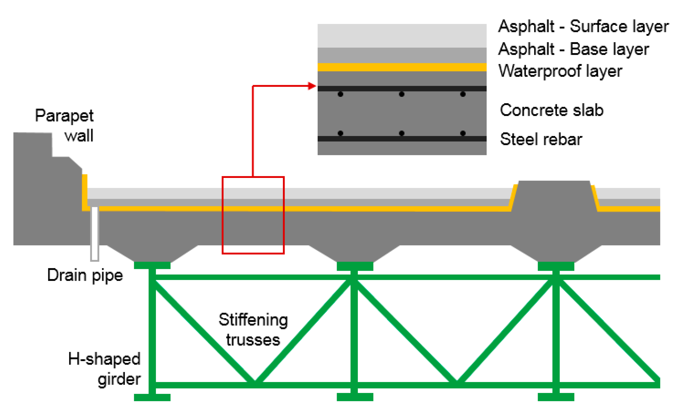
The most popular road bridge structure in Japan is the steel girder bridge with reinforced concrete slab. An reinforced concrete (RC) deck slab consists of four main layers: the concrete slab, the waterproof layer, the asphalt surface layer, and the asphalt base layer (
Figure 1). Since a waterproof layer is not mandatory in Japan, waterproof layers are not installed in at least 20% of RC deck slabs in national roads. The total thickness of the two asphalt layers is around 70 mm to 80 mm.
These structural features are standardized to resist the normal Japanese environment and a certain degree of climatic variation. Moreover, this design is durable enough to handle the mechanical damage caused by traffic loads. However, it does not have enough resistance to severe environments. One degradation phenomenon often observed is rust juice from cracks caused by de-icing salt. Normally, NaCl is used for de-icing. In Japan, the problem of de-icing salt damage increased after the prohibition of studded tires on April 1991. Two years before this prohibition, the amount of de-icing salt used on national roads in East Japan was around
. From 2006 to 2008, this figure increased by a factor of 4.1, to around
in average, or
per
of road [
16]. The Japanese design code for bridges does not account for such high salt concentrations, and thus they pose a threat to existing bridges.
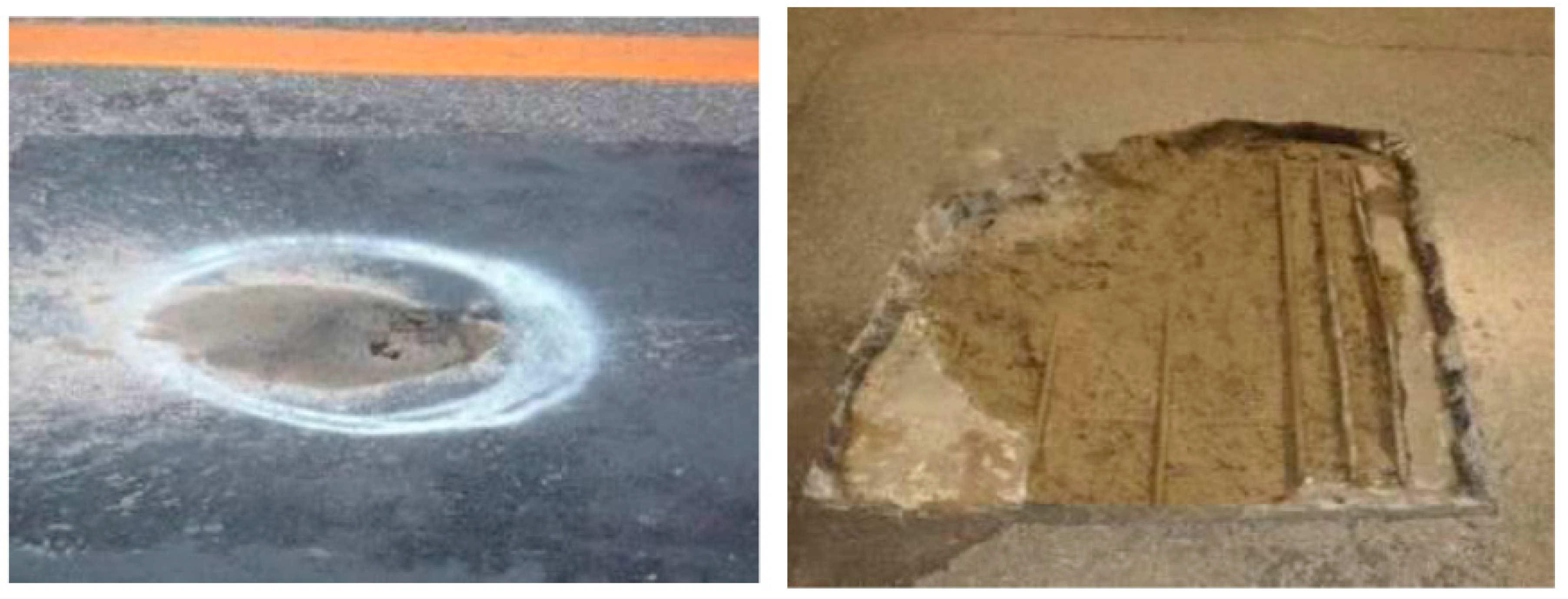
To date, there have been many examples of complex deterioration in bridges in East Japan.
Figure 2 gives a typical example, which was provided by the Ministry of Land Infrastructure and Transport East Japan Regional Development Bureau. The bridge was used for 36 years, and the average traffic volume was only 12,000 vehicles per day, but serious deterioration occurred [
17]. The proposed mechanism is as follows. As Matsui (1987) found, when salt water enters the crack, freezing and thawing, alkali silica reaction (ASR) and rebar corrosion begin to occur. Therefore, cement paste parts are seriously damaged. As a consequence, bending and shear capacity are significantly reduced, and shear punching failure takes place [
18]. Additionally, soluble components such as Ca(OH)
2 and Na
2SO
4 dissolve in water and combine with carbon dioxide in the atmosphere, resulting in efflorescence. The appearance of efflorescence indicates a high probability of crack penetration and water invasion; thus, it is an important degradation indicator in concrete inspection.
3.2. Data Arrangement and Description
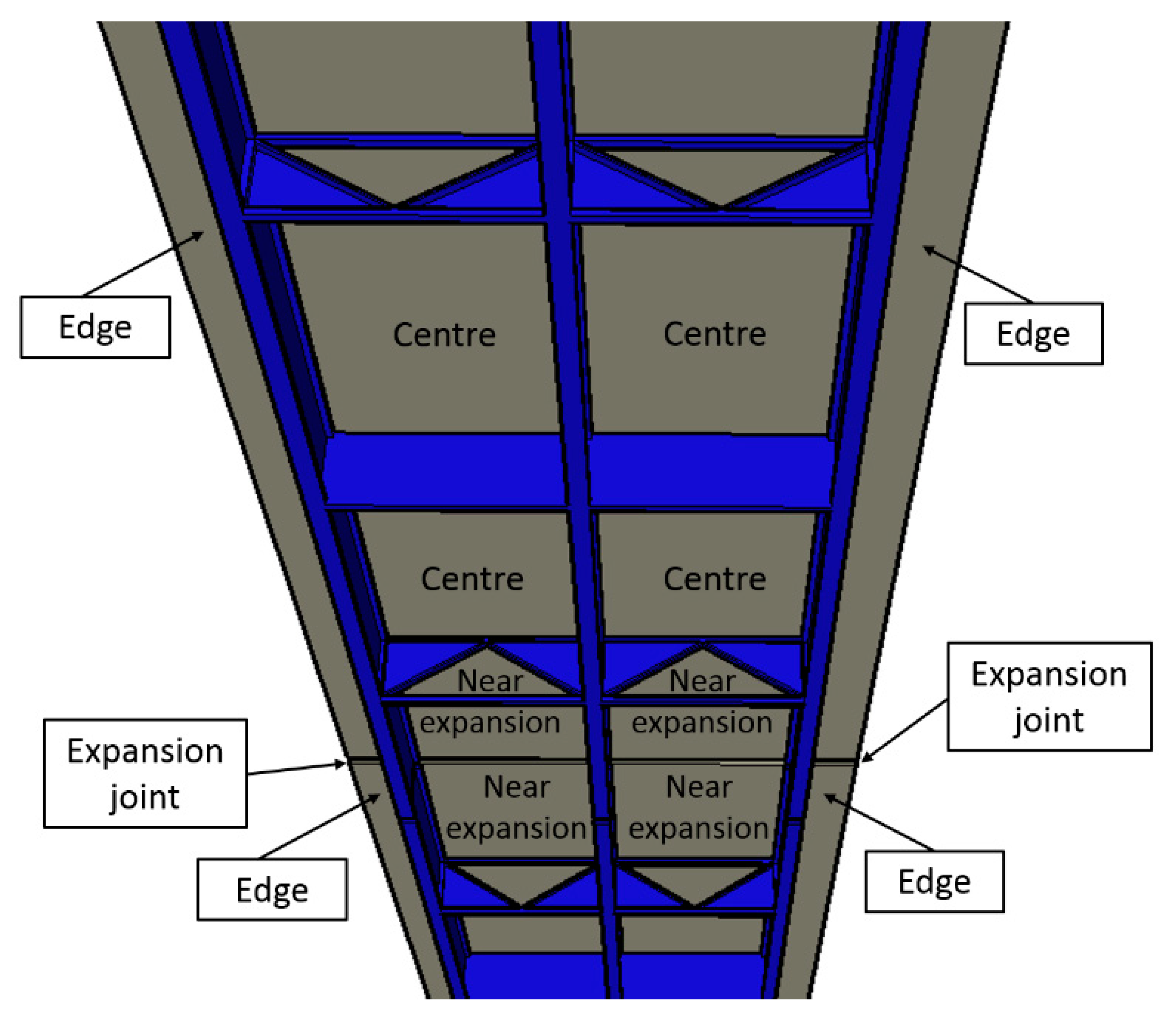
The analysis object of this study was the bridge panel, which is defined as the slab area surrounded by the main girders and cross girders, as shown in
Figure 3. Each deck slab featured multiple panels, which were considered independent objects. Studies have shown that panels in different positions show different deterioration rates. Consequently, the panels were separated into two groups, depending on whether they were in the center of the slab.
The inspection standard for RC deck slab panels is shown in
Table 1. The panel condition is classified into five categories, from sound to damaged. An RC deck slab is defined as ‘failed’ if the rating is C or worse in this analysis. This condition is defined as the occurrence of an event in the survival analysis. As previously explained, water leakage and efflorescence strongly accelerate the progress of deterioration. Thus, this threshold is reasonable for defining the event.
For the dataset, national road inspection data were used. Since the data were obtained from the current maintenance database, influential factors affecting slab deterioration such as poor material properties (shrinkage), inadequate pouring procedures, etc. is not available. So, as the first step, we only focus on structural features and environmental conditions. In Japan, national roads are maintained by the local MLIT bureau. Inspections began only in 2003; thus, if a bridge was constructed in 1960, the first inspection was over 40 years after construction. Therefore, the earlier the construction year of the bridge, the longer the time before the first inspection, which means that the survival time cannot be obtained precisely. To mitigate the impact of this long blackout period while ensuring a reasonable amount of data, and also because repairs (which affect the precision of survival time calculations) were frequently conducted before 1980, only bridges constructed after 1980 were included in our dataset. In addition, environmental data such as precipitation, which are published by Ministry of Land, Infrastructure, Transport and Tourism, are available only from 1980.
In Yamazaki et al. (2015), if one bridge component was inspected multiple times, the continuous inspection record was treated as several independent data [
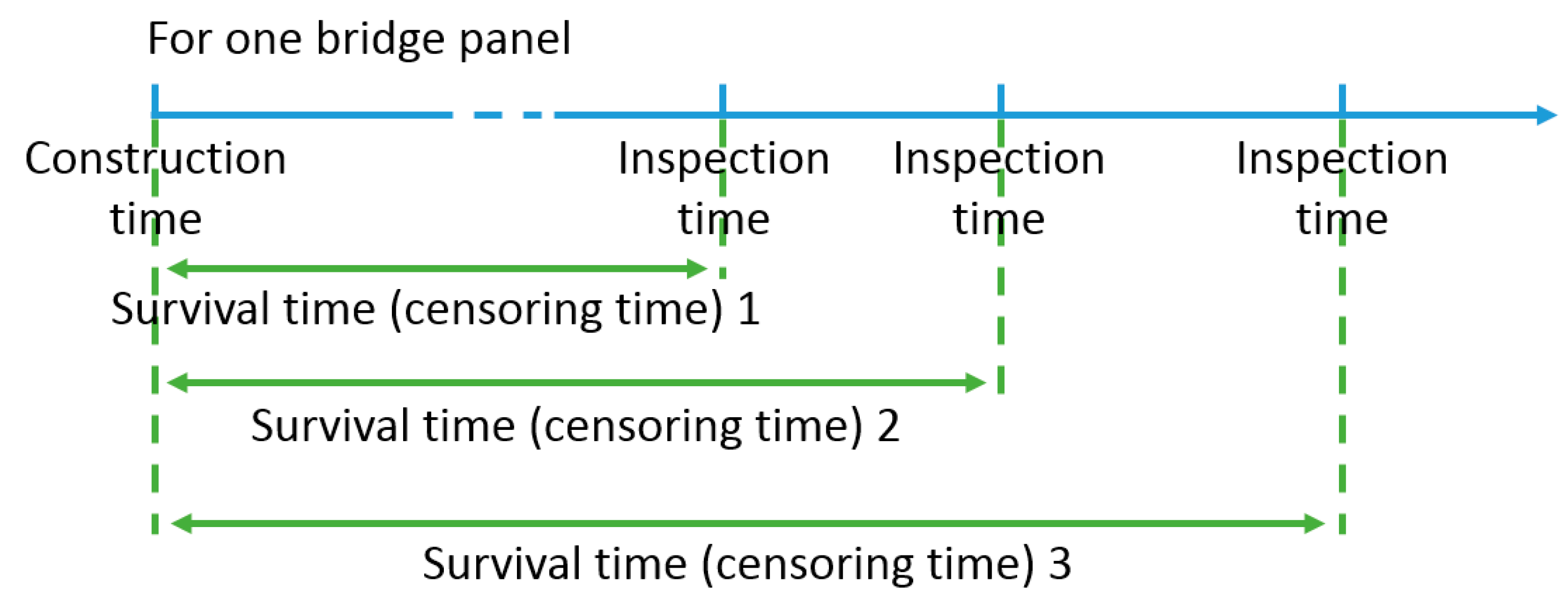
7]. Therefore, each component could have several survival times (or censoring times). For example, as
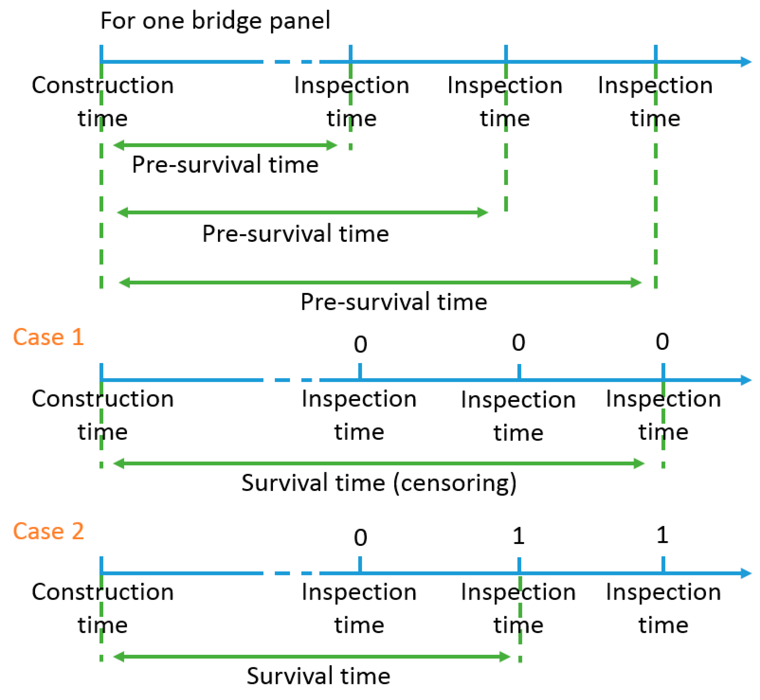
Figure 4 shows, if a panel was inspected three times, there are three survival times (or censoring times) in the dataset. This assumption is convenient for data sorting. However, theoretically, from the definition of the basic concept, one element can have only one survival time or censoring time. Thus, the previous data sorting method contradicted the basic concept of survival time.
To obtain a more rational survival time (or censoring time), each continuous observation of each object was first treated as a separate datum, and pre-survival time was calculated as shown in
Figure 5. One pre-survival time was then selected as the true survival time. As Case 1 shows, 0 represents the non-occurrence of the event, and 1 represents its occurrence. For each panel, if the event did not happen in the inspection period (all of the data are censored), the period between the construction time and latest inspection time was the survival time (properly speaking, the censoring time) of this object. For case two, if the event occurred, the period between the construction year and the time the event first occurred was the survival time.
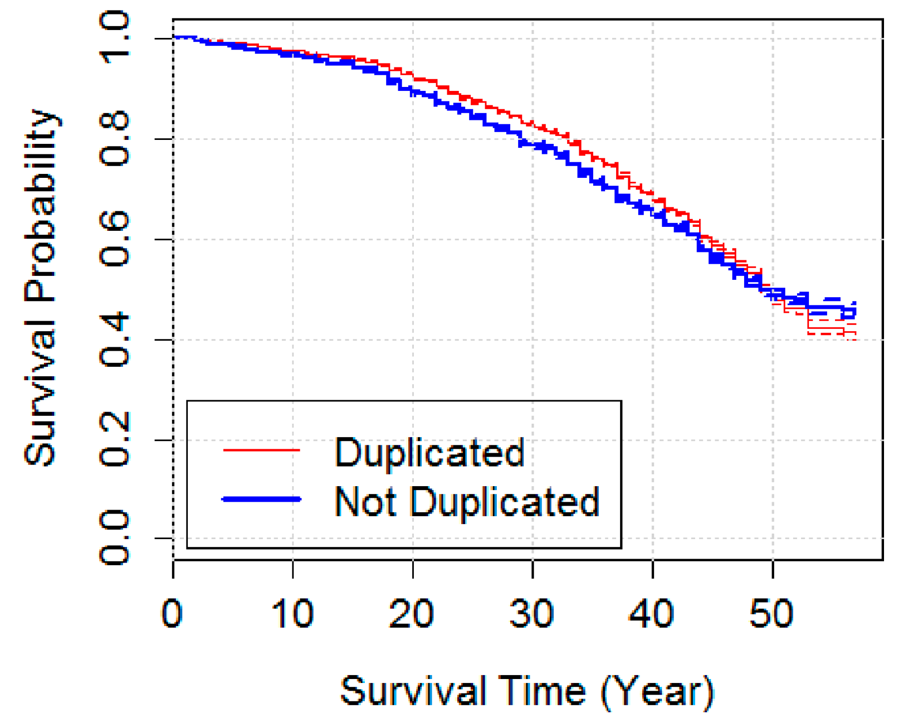
Multiple survival times or censoring times for one object lead to redundant data, which could lead to imprecision in the KM curve and incorrect multivariate analysis results.
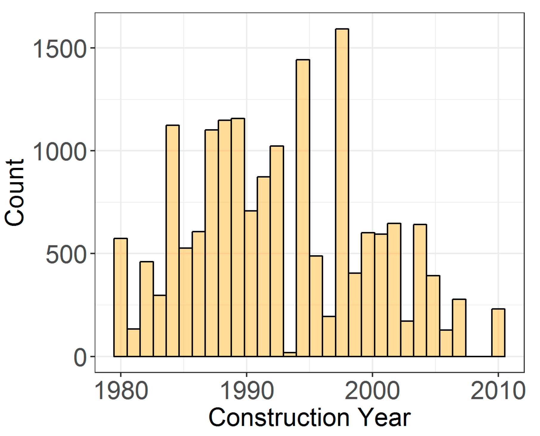
Figure 6 shows the result of comparing KM curves; the red line presents the KM with redundant data, and the green line presents the KM curve after data cleaning. The dotted line shows the 95% confidence interval. It can be clearly seen that after data cleaning, the declination of the KM curve changed, indicating that the data cleaning process was necessary. Before data cleaning and sorting, the dataset included inspection data for 82,016 panels in 525 steel girder bridges. After selection and cleaning, our dataset included 17,557 panel inspection records for 183 bridges. The construction year distribution is shown in
Figure 7.
Multiple variables relating to bridge slab deterioration were used as explanatory variables. Structural features and environmental conditions including precipitation over four seasons, winter temperature, etc. were considered and selected as variables. National Land Numerical Information published by the Ministry of Land, Infrastructure, Transport, and Tourism was used for weather data accumulation. These data were generated from observations by the Japan Meteorological Agency between 1981–2010. The resolution of these covariates is a
mesh, and they were numerically analyzed to correct for the effects of topography and elevation. Using Rstudio Version 1.0.143, and referring to the bridge coordinates added by Iwaki et al. (2013), this National Land Numerical Information was combined with inspection records [
10].
However, precise multivariate analysis results are difficult to obtain due to high correlation between some variables. In our dataset, environmental data such as precipitation over four seasons and winter temperature were highly correlated; therefore, without appropriately selected variables, univariate and multivariate analysis led to paradoxical results. For example, a univariate analysis of precipitation over four seasons showed an increase in the hazard ratio, while multivariate analysis showed that the risk of some variates tended to decrease. This unexpected result implies that the selection of an appropriate explanatory variable was a precondition for obtaining good results. In this analysis, the correlations of all of the variables below 0.5 were selected as explanatory variates.
The covariates used in analysis are shown in
Table 2. They were recorded as numerical and categorical covariates. All of the numerical covariates were standardized and are presented in the methodology section. Additionally, the unit, mean value, and standard deviation of all of the numeric variables are shown in the table. For categorical covariates, the crossing condition, panel position, slope, de-icing salt usage, and waterproof layer installation situation were separated into different groups. The definition for each group is also shown in the table. List-wise case deletion was executed for records with insufficient information.
In addition, as stated earlier, the inspection years of the data were 2003 to 2013, which is more than 20 years later than the construction years. Thus, some groups constructed earlier show longer survival time distribution. To solve this problem, the Cox stratified model was introduced to the analysis. This model allows a factor to be adjusted for without estimating its effect. The construction year was stratified in this analysis. For parameter estimation, if the data are stratified for g groups, the likelihood function can be written as follows:
is the likelihood from stratum
g.
4. Results for East Japan
In
Figure 6, the red line represents the KM curve of all of the panels. Survival probability declined to 50% after approximately 25 years, implying that the deterioration rate is faster than in the Tokyo region, as shown in
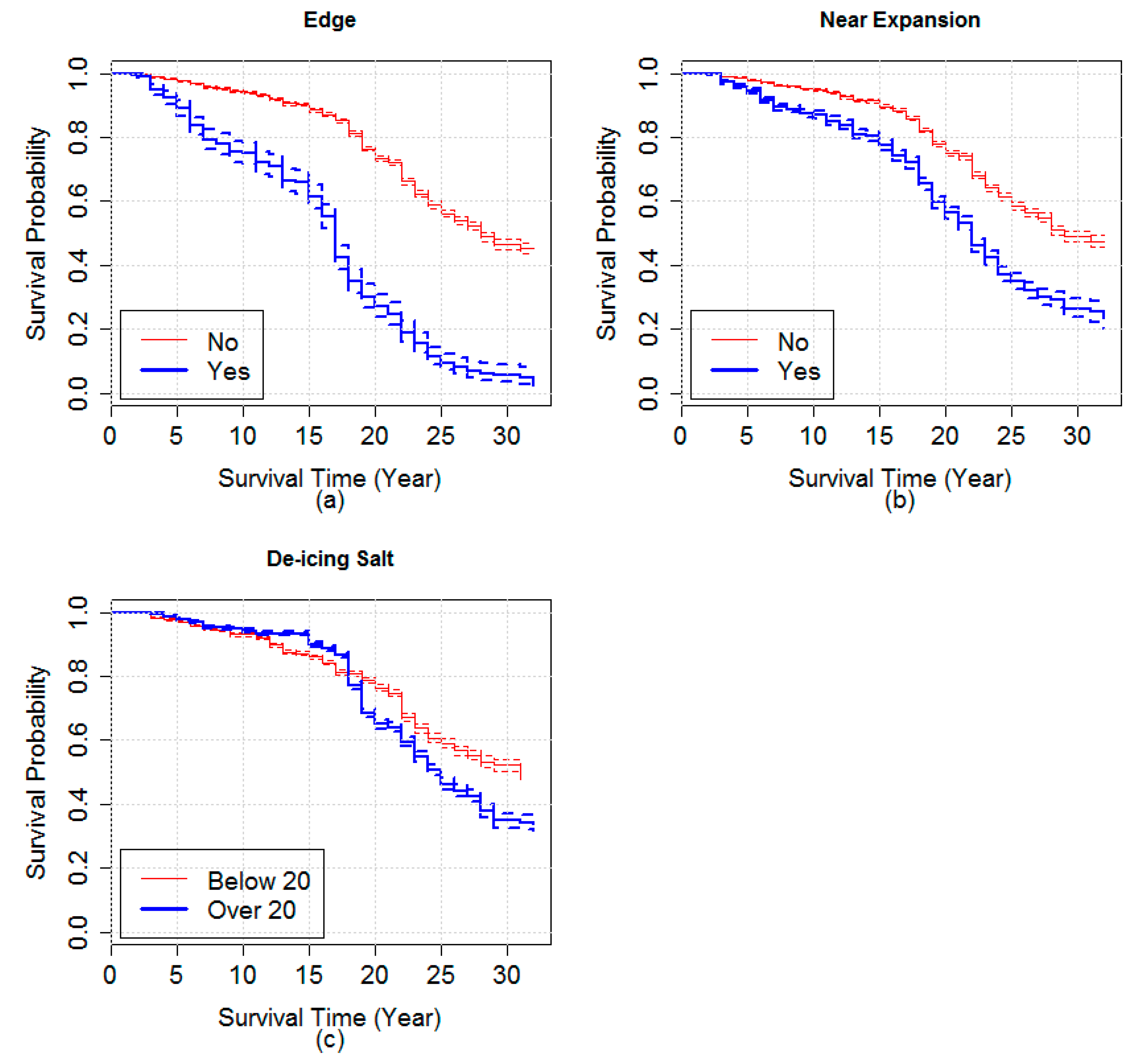
Section 5. The representative KM of some category variables with very different survival probability declinations are shown in
Figure 8.
Figure 8a shows results based on whether panels are on the edge.
Figure 8b shows results based on whether the panels are positioned near the expansion joint.
Figure 8c presents the survival probability of two de-icing groups, below and above 20 t/km. The survival probability declination of these variables was found to be very different, indicating that these factors could strongly affect the deterioration rate.
The univariate analysis gave us a general understanding of the explanatory variables, separately and on one side. The KM curve confirmed the basic information of each category description variable and roughly plotted the deterioration rate. However, to evaluate the effect of all of the factors and determine the relationship between all of the explanatory variables, a multivariate analysis was performed; the result is shown in
Table 3.
The hazard ratio is interpreted as the ratio of the possibility of degradation over any time duration. The
p value is from the Wald test, and determines the significance of the results. The equation is as follows:
Essentially, it tests whether is statistically equal to . In this analysis, always equals 0 because the hazard ratio is calculated using . Therefore, the p value indicates whether significantly contributes to the hazard ratio.
For numerical explanation variables, an increase in traffic volume slightly increased the hazard ratio. Moreover, the average slab thickness in East Japan was 22.4 cm, and the hazard ratio of the slab thickness was close to 1; the
p value also showed that
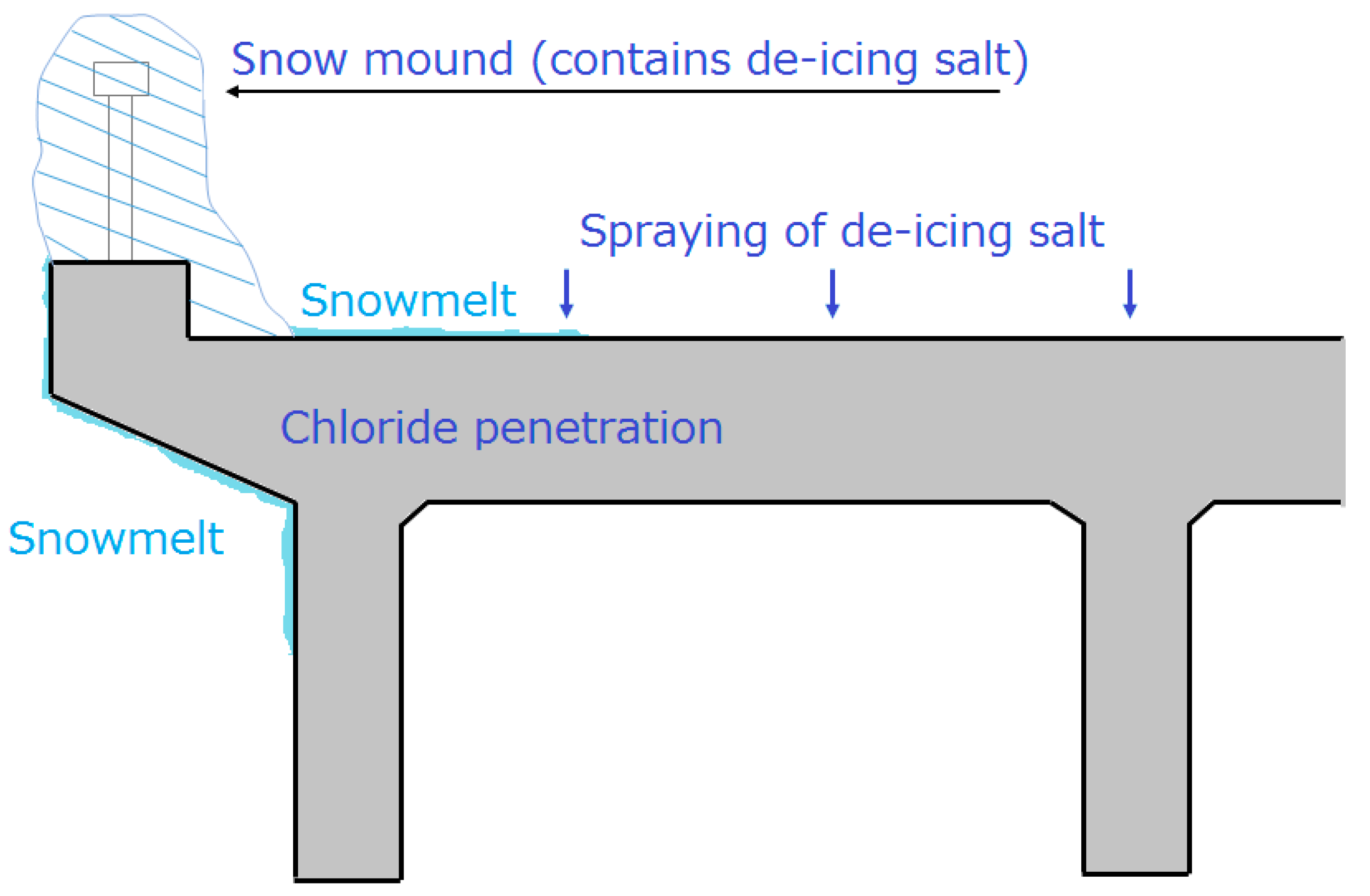
did not make a significant contribution to the hazard ratio. This result implies that fatigue damage was not a major reason for the deterioration of the bridge slabs. However, winter precipitation and high de-icing salt usage greatly increased the risk of deterioration. The reason is shown in
Figure 9. Due to heavy snowfall and snow removal, snow accumulated at the edge of the slab and became a snow mound. The snow mound melted little by little, and during this process, snowmelt with a large quantity of de-icing salt penetrated the crack, keeping the slab in a condition of consistently high humidity and salinity and resulting in further cracking and steel corrosion. Therefore, deterioration greatly accelerated.
Overpasses showed a smaller hazard ratio from the engineering point of view, while bridges constructed across rivers had relatively high humidity. Different panel positions had different hazard ratios. Panels near the expansion joint or edge showed high risk, as water could easily contact the slab area through the expansion joint and penetrate the concrete near the edge of the slab, causing steel corrosion and concrete spalling. Slabs with waterproofing showed lower risk, meaning that a waterproof layer could improve slab durability. These results indicate that waterproofing should have been improved at the edge of the slab to increase durability. In addition, they show that a sloped slab had a lower risk, as water could not easily accumulate on it.
The hazard function for survival analysis with multiple variates is defined as
.
is called the baseline hazard. The baseline hazard does not depend on covariates; instead, it depends on time.
, which is called the risk score, is the total risk for each bridge. In other words, if the bridge has a large
, it statistically has a high deterioration risk.
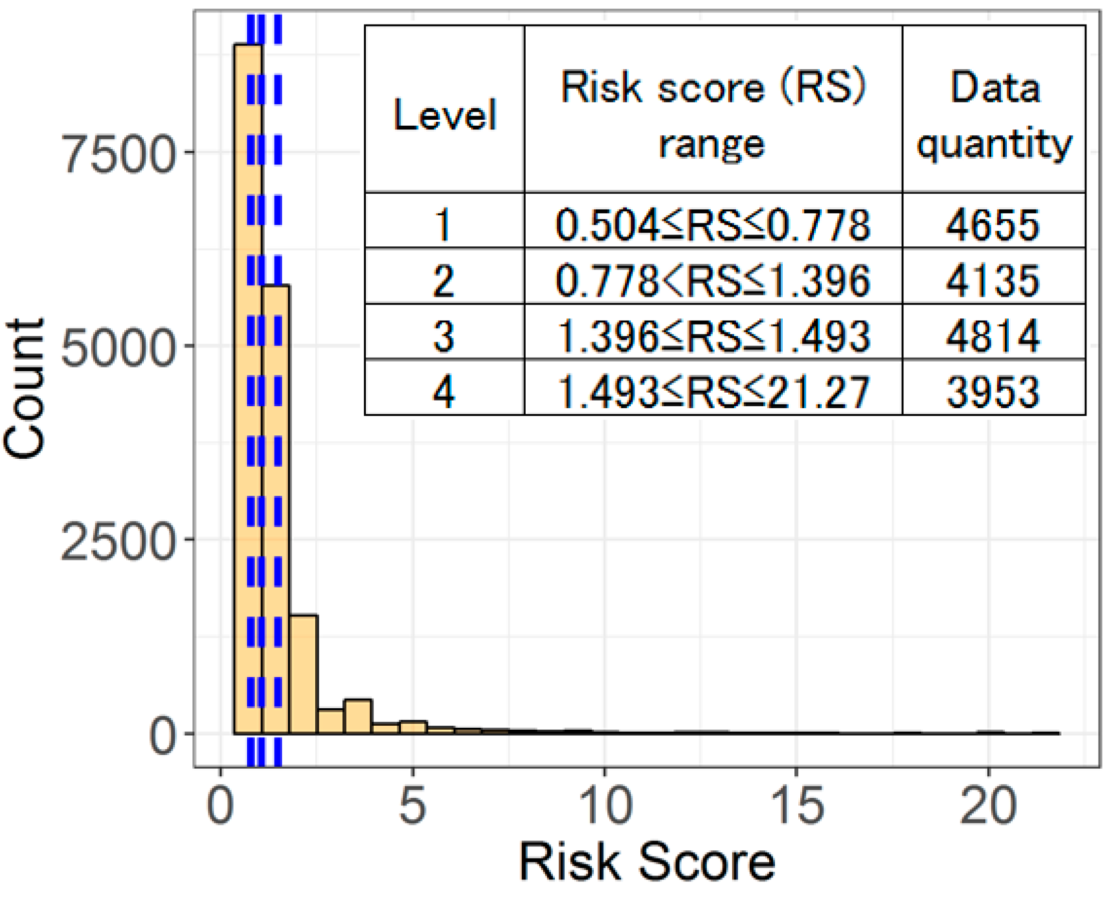
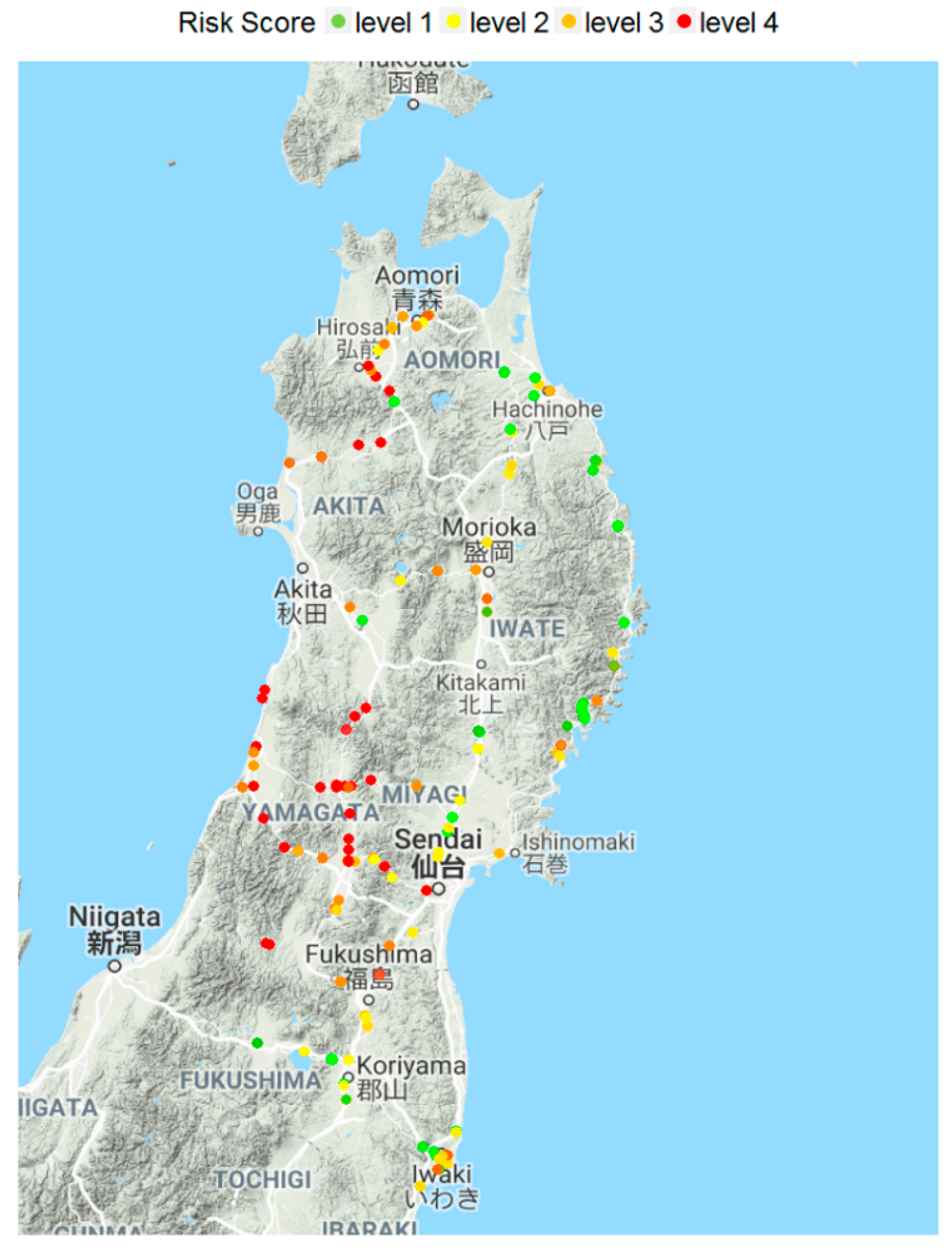
Figure 10 gives the risk score distribution of all of the bridge slab panels. The risk scores were then divided into four approximately equal parts. The table within the figure shows the risk score range and data quantity of each level. Using the geographical coordinate information, risk scores were plotted in Google Maps (see
Figure 11). The risk scores increase as the colors change from green to red. The Japan Sea side shows a higher deterioration risk than the Pacific side. Geographically speaking, East Japan is divided into the Japan Sea and Pacific sides along the Ou Mountain Range. As the dry seasonal wind from the north crosses the Japan Sea, it absorbs moist air, and clouds form. This moist air cloud is further enhanced by the ascending air current as it passes over the Ou Mountain Range, and more snow is precipitated during the process. After crossing the mountain range, it becomes dry air, and reaches the Pacific side. Therefore, snows are very heavy on the Japan Sea side, and a large amount of anti-freezing agent spray is required. On the Pacific side, because the air is relatively dry, there is less rain and snow. The results indicate that the bridge deterioration was highly influenced by weather conditions.
5. Deterioration Features and Data Description of the Tokyo Region
5.1. Deterioration Features of the Tokyo Region
The Tokyo expressway is over 330 km long and is under the control of Metropolitan Expressway Co., Ltd. Inspection data on parts of the Metropolitan Expressway’s steel bridge deck slab, the Route 3 Shibuya Line and Route 5 Ikebukuro Line, were used for analysis. The construction years of both routes comprised around 1965 to 1975. By processing longitude/latitude coordinates and the management ledger, a detailed environmental/structural dataset was prepared.
Fatigue damage caused by repetitive vehicular traffic is the main reason for RC slab deterioration in the Tokyo region (Matsui et al. (1986) [
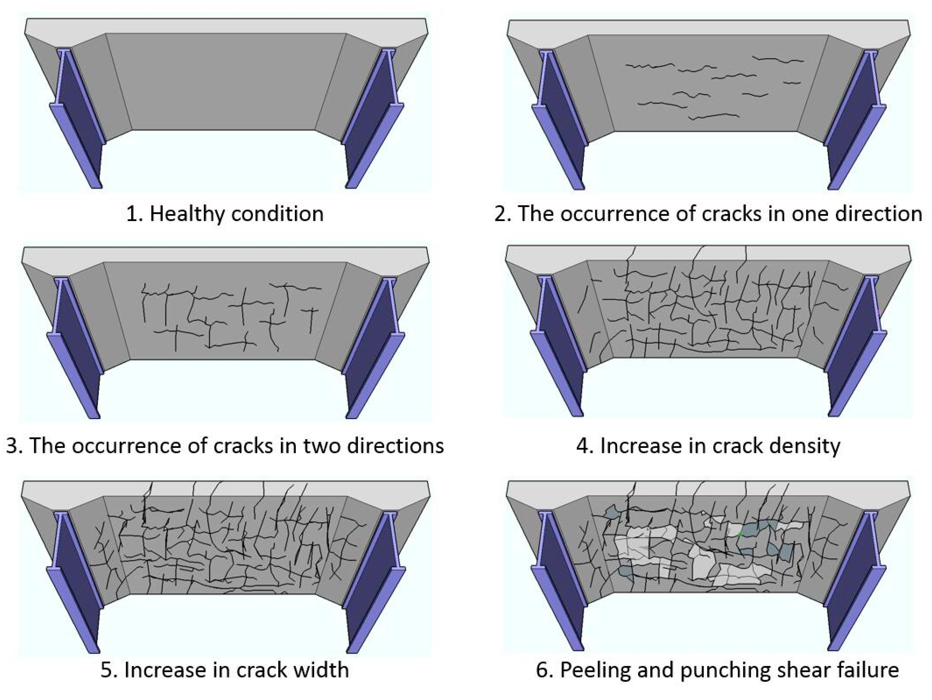
19]). After decades of use, these slabs have deteriorated a great deal. Usually, during visual inspection, one and two-dimensional cracks, water leakage, and efflorescence were observed on the bottom of the slab. As Matsui (1987) stated, in the initial state, deterioration of the slab starts with the appearance of transverse cracks, which is considered as related to shrinkage and construction joints. Since they undergo a heavy traffic volume of around 45,000 vehicles per day on average, transverse cracks gradually increase, and longitudinal cracks also start to appear. As two-dimensional cracks develop further, mesh cracks can be observed. Then, as crack density and crack width increase, punching shear failure ultimately occurs. The process is shown in
Figure 12. As stated earlier, during this process, water such as rainfall significantly accelerates the deterioration process. In addition to the development of two-dimensional cracks, the interlock effect becomes weak, and shear capacity is decreased. Eventually, punching shear failure occurs. According to this theory, a quantitative deterioration assessment has been done by Eissa et al. (2018) to predict the remaining fatigue life of bridge decks based on their site inspected cracks [
20,
21]. However, the research is based on mechanics aspects, which did not consider the environment effect. Therefore, this research can be considered a risk assessment by integrating both mechanics and ambient effect. As in East Japan, other factors such as structural features (slope, slab thickness, etc.) also affect the slab degradation rate.
5.2. Data Arrangement and Description
The inspection standard for highway RC deck slab panels is similar to East Japan. An RC deck slab is defined as ‘failed’ if two-dimensional cracks and the appearance of efflorescence at the bottom of the slab was observed. This is also the definition of an event in survival analysis, since these phenomena signify the appearance of penetration cracks and water invasion. Under this condition, further deterioration is highly accelerated. Thus, on the basis of the inspection standard, the event was defined as occurring when the slab condition reached this level or worse. This definition correlates with the event definition for the East Japan region. Event occurrence indicates that accelerated deterioration will occur due to a lack of (or inappropriate) repair and rehabilitation. The survival time calculation, data selection, and cleaning process were the same as for East Japan. However, the management level in the Tokyo region was relatively high; repairs were frequently conducted. According to our Tokyo dataset, 49.8% of the panels had been repaired and reinforced.
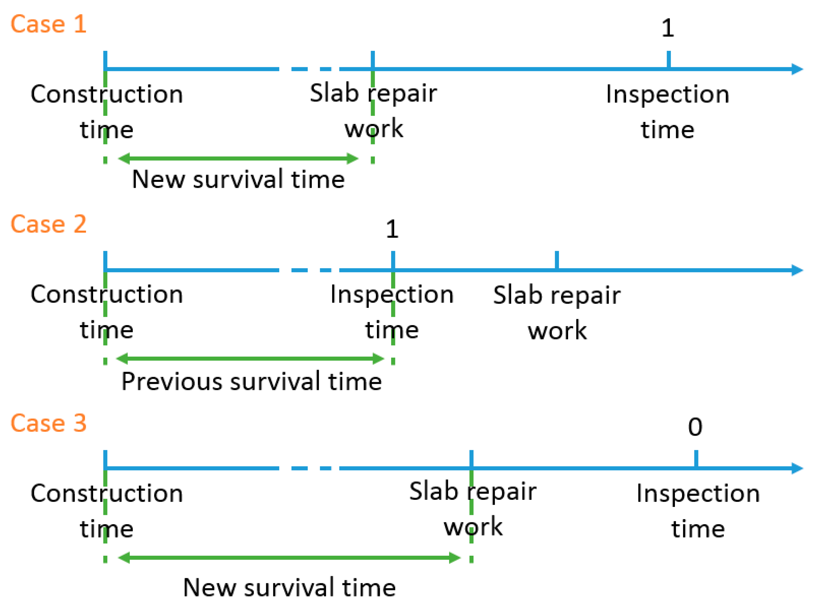
Table 4 shows repair work in the Tokyo region. If repair was conducted before inspection, the condition of bridge panels would already be improved, greatly changing the deterioration rate and introducing inaccuracies into the analysis. Therefore, it was necessary to consider the repair effect. If the repair work included crack injection, steel plate bonding, replacing and carbon fiber reinforcement, the occurrence of the event was assumed. According to this assumption, if these slab repairs were conducted, a complementary survival time was calculated. These complementary survival times were then compared with the survival times previously obtained. As
Figure 13 shows, if it was shorter than the previous survival time, the complementary survival time was chosen as the object’s new survival time (Case 1). If not, the previous survival time was reserved as analysis time (Case 2). Moreover, if the data had only a censoring time (indicating the event had not occurred by inspection time) but repair work, which is shown in
Table 5, was conducted, the complementary survival time replaced the censoring time (Case 3). The original dataset contained 71,888 data points; after cleaning and selection, 27,041 data points were left.
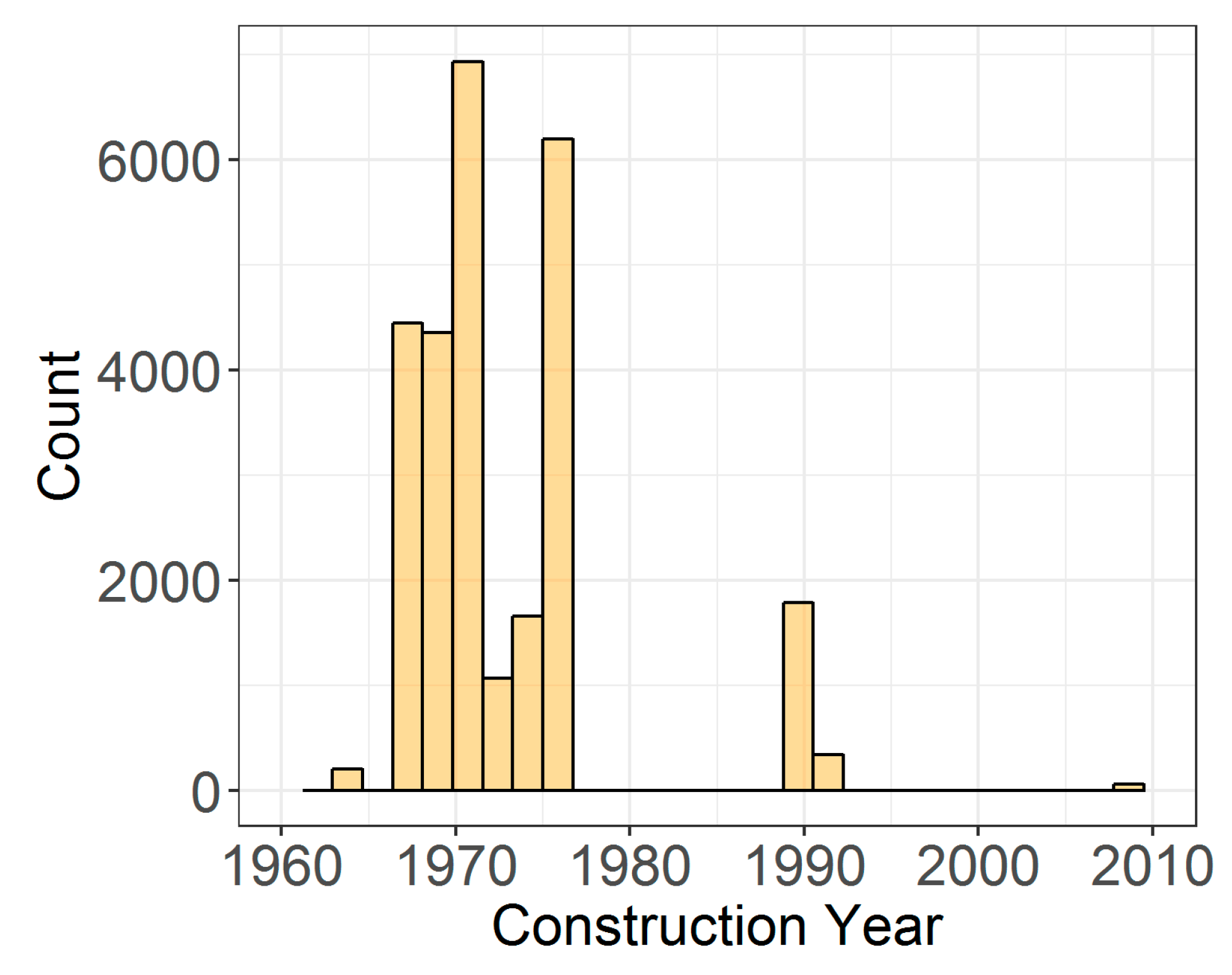
Figure 14 shows the construction year distribution of all of the panels.
Variables used in the analysis are shown in
Table 5. As for East Japan, the mean value and standard deviation of numeric covariates and detailed definitions of category covariates are also shown. The selection process was the same as for East Japan. The National Land Numerical Information published by MLIT was used for weather data accumulation. As already stated, the bridges of these two regions are governed by different organizations; therefore, the inspection systems are different. East Japan bridge inspection mainly focuses on water leakage and efflorescence. However, Tokyo region bridge inspection not only focuses on efflorescence, it also pays attention to crack density. Therefore, some variables in the dataset were different than for the East Japan dataset. Traffic volume, structural features, panel position, design code, and precipitation were used as variables.
Design codes were divided into two groups: the first for design codes from 1964 and 1956, and the second for those after 1964 (1973, 1980, etc.). The reason for this division is that major reforms in mechanical resistance specifications occurred after 1964.
Table 6 compares the minimum ratio for the distributing bar and slab thickness between different design standards. It can be clearly seen that the amount of the distributing bar specified increased after 1964. Additionally, the minimum slab thickness increased after 1973.
Currently, judgment of the cause of deterioration depends on bridge engineers’ experience and skills. However, visual inspection and sound testing are inefficient and rely too much on inspectors’ personal judgment. In many cases, it was difficult to identify a single factor responsible for deterioration. In such cases, deterioration was simply recorded in the inspection ledger as ‘complex deterioration with multiple deterioration factors’. This method would not contribute to efficient maintenance based on the structural and environmental conditions of individual bridges. Thus, identifying predominant risk factors is urgently necessary.
6. Results for the Tokyo Region
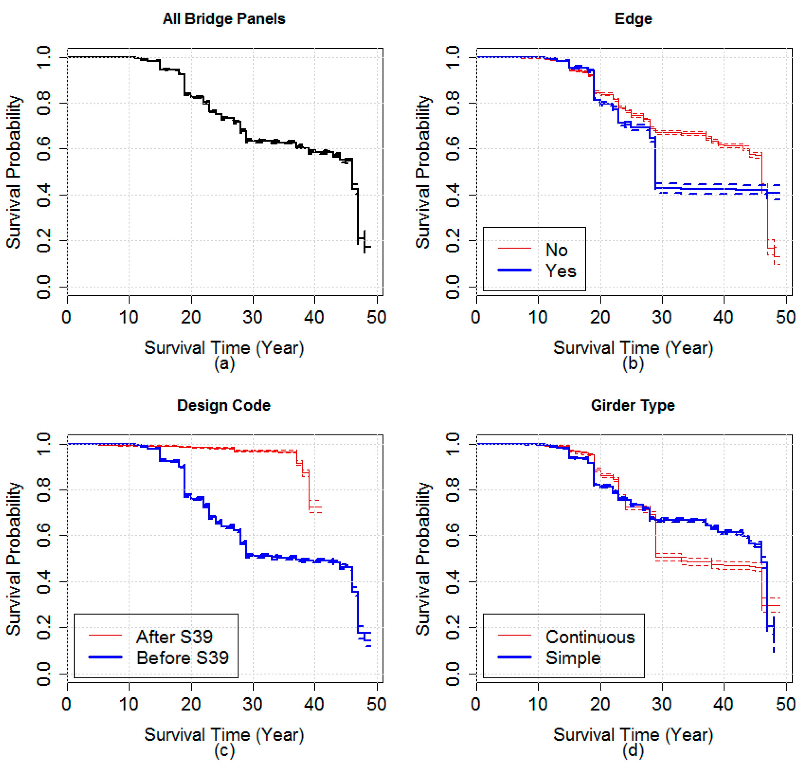
Figure 15a shows the survival probability of all of the bridge panels. The survival probability fell to 50% in 45 years.
Figure 15b–d show the survival probability of three category explanation variables: edge, design code, and girder type. For each variable, each group shows a different declination trend, indicating that these groups affect the deterioration rate. In particular, a large gap between design codes is shown in
Figure 15c, which reveals that safety was greatly improved by the design code overhaul after 1964. Kawai et al. (2016) also stated that according to their analysis, slabs designed before 1964 showed shorter fatigue life [
22].
The multivariate Cox regression analysis result is shown in
Table 7. Unlike the East Japan results, risk increased more than 30% when traffic volume increased by one standard unit. From the engineering point of view, a slab undergoing frequent wheel load from traffic reaches its fatigue limit faster. However, increasing the slab thickness decreased the risk, because a thick slab has enhanced loading capacity. According to our data, the average slab thickness in the Tokyo region was only 19.8 cm. Thus, unlike in East Japan, repeat traffic loading was a major factor in deterioration. These results reveal that slab thickness should be increased to resist traffic load.
As in East Japan, the risk decreased as the slope increased because of faster water runoff. Moreover, winter precipitation showed high risks. Since winter precipitation was highly correlated with precipitation in other seasons, this result indicates that precipitation increased the deterioration rate. As in East Japan, slabs usually have a longer lifespan under relatively low ambient humidity. Okada et al. (1982) pointed out that the degradation rate of reinforced concrete slabs was faster if water was present. If water has sufficiently penetrated the cracks of a concrete slab, there is a possibility of fatigue fracture even under the design load, which is about one fifth of the static stress [
23]. Water penetration through cracks probably promotes scratch polishing and high water pumping pressure on the cracked surface, and rapidly increases crack width. Thus, in both East Japan and the Tokyo region, slab deterioration is significantly influenced by water.
Panels at the edge of the deck tended to have a higher likelihood of deterioration, because these panels were more frequently in contact with water such as rainfall. The report from the Chugoku Regional Development Bureau (2016) also revealed that deterioration of the edge of the slab was more serious than in the center [
24].
The results also show that continuous girders had a lower deterioration rate. From the engineering perspective, continuous girders are safer because they have fewer expansion joints. Thus, water has less opportunity to penetrate and contact the unprotected part of the slab. However, as
Figure 15d shows, the survival probability declination of continuous girders was faster. In the specifications for highway bridges [
25], the minimum slab thickness designation for continuous girders is smaller than for simple girders, as
Table 8 shows.
In terms of the design code, the slab panels constructed according to the Specifications for Steel Highway Bridges issued in 1956 and 1964 showed high risk, indicating that a small amount of distributing bar and thin slab thickness greatly decreases the safety of slabs.
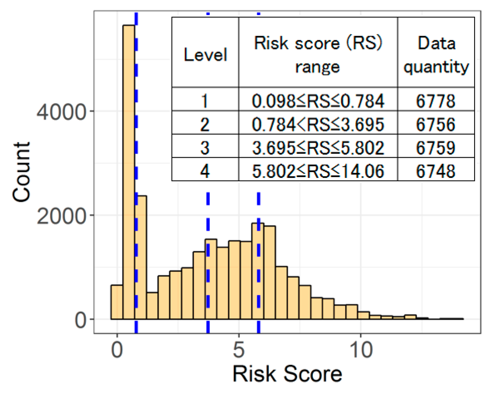
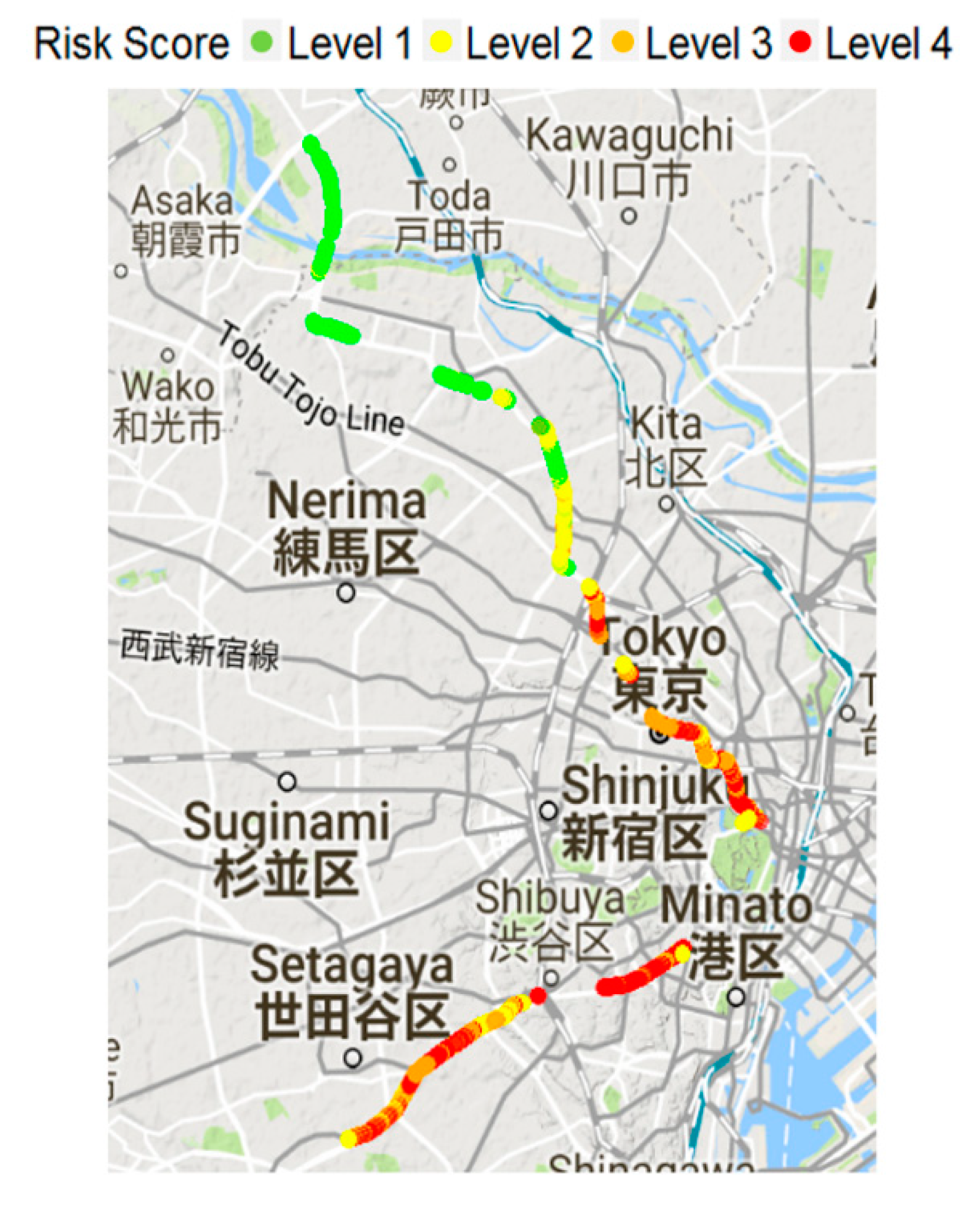
Figure 16 shows the risk score distribution of all of the bridge slab panels. Risk scores were again divided into four approximately equal parts. The table within the figure shows the risk score range and data quantity of each level. Using the geographical coordinate information, risk scores were plotted in Google Maps, as shown in
Figure 17. In the north area, risks were relatively low, but in the central and south parts of Tokyo, risks were high, as the traffic volume in those areas is relatively high. Additionally, most slabs in this area were constructed according to design codes prior to 1964. By referring to the risk score map, a manager can easily determine which part is at high risk. Therefore, the efficiency of inspection and rehabilitation can be improved, and optimal construction decisions can be made.
7. Conclusions
In this study, visual inspection data of bridge panels in East Japan and metropolitan Tokyo highway bridge panels were used for survival analysis in order to facilitate optimal maintenance decision making. First, unlike in previous research, a data cleaning process was used; then, by considering the effect of repair work, the precise survival time of each bridge panel was obtained. After correlation checking and variable selection, a KM curve estimator was used to clarify the basic information of important variables. Cox regression was then applied to identify the hazard ratio of each variable. The results can be summarized as follows.
First, the different deterioration characteristics of different regions were clarified. Reduplicative dynamic traffic load was a major reason for the deterioration of bridge deck slabs in the Tokyo region. However, it was not a high risk in East Japan, because the traffic volume there was not as high as in the Tokyo region. Correspondingly, thicker slabs had much greater loading capacity; therefore, a decreased hazard ratio was evident in the Tokyo region. In East Japan, because of lower traffic volume and thicker slabs, slab thickness was not a major deterioration factor.
Second, water including winter precipitation increased the deterioration rate in both regions. Especially in East Japan, during the extended snow melting process, salt water penetrates into cracks and accelerates the deterioration process. Under this condition, rebar is corroded and slab is seriously damaged unless there is appropriate protection and repair work. Correspondingly, water flow is faster for slabs with greater slopes; thus, the hazard ratio tends to be smaller. Moreover, waterproofing in East Japan reduced risk, indicating the importance of preventing water from penetrating the slab.
Third, panels in different positions had different deterioration rates. Usually, the panel on the edge of the slab or near the expansion joint had high risks because of the high possibility of contact with water. In Tokyo, even panels in the center of the slab that directly carried heavy traffic loads had a smaller hazard ratio than the edge area. In addition, for both areas, because the water flow was more rapid with a greater slope, the hazard ratio was small. These results statistically prove that water plays an important role in deterioration. Therefore, waterproofing on the edge should be enhanced against severe environments.
Fourth, using geographical coordinate information, risk scores were mapped; distinctions between high-risk and low-risk areas were shown. In East Japan, due to its special geographical environment, the Japanese seaside is snowy in winter, resulting in the use of large amount of de-icing salt. Therefore, the deterioration condition and rate in this area is relative high. In the south of the Tokyo region, since traffic volume in those areas is relatively high and most slabs in this area were relatively thin according to design codes prior to 1964, the total risk score is high. As a result, through this quantitative multiple deterioration factors assessment, the priority of maintenance in the case of an insufficient budget will be determined by more accurate statistical analysis rather than personal subjective judgment. Briefly speaking, it can be applied to optimize decision-making. Therefore, under the premise of ensuring more efficient and accurate countermeasures, financial burdens can be lessened.
In this study, the risk factors for bridge deck slab components were quantitative evaluated. The results for these two typical regions can be extrapolated to the entirety of Japan and used for optimal decision making. By considering the content and quantity of risk factors, deterioration patterns can be clarified. Therefore, design, maintenance and rehabilitation can be rationalized.
In future research, the amount and quality of covariates should be enhanced in order to improve the analysis precision. For example, some initial variables that significantly affected the speed of deterioration, such as the material properties (shrinkage), inadequate pouring procedures, concrete mixture, and depth of concrete cover were not recorded, so we did not consider these factors. By cooperating with authorities, we can retain and digitize this information for future data-driven bridge maintenance. In addition, for existing covariates, we must improve the data quality to accurately evaluate risk factors; for example, it would be a significant step forward if we could simulate the freeze–thaw cycle by calculating factors such as the concrete surface temperature.


