Relative Intensity Noise of Hybrid Mode-Locked Bound Soliton Fiber Laser: Theory and Experiment

Featured Application

High repetition rate optical bound-pulse generation with low relative intensity noises.

Abstract

Relative intensity noises (RIN) of mode-locked lasers are properties which are crucial for applications. In the literature, there have been plenty of theoretical/experimental studies on the RIN noises of passive/active single-pulse mode-locked lasers. Since some mode-locked lasers can also be operated under the bound-pulse mode-locking state, it is thus very interesting to further examine the RIN properties under bound-pulse mode-locking, and to verify if there are possibilities for RIN noise reduction as predicted by some previous theoretical works. The conventional analytical formula based on the soliton perturbation theory can no longer be applied due to the pulse shape complexity for the bound-pulse mode-locking cases. New theoretical tools for modelling general mode-locked lasers are eagerly awaited. In the present work, the RIN noises of an environmentally stable 10 GHz hybrid mode-locked Er-doped fiber laser capable of bound-soliton generation are experimentally investigated, and a novel theoretical method based on the linearized backpropagation approach is theoretically developed for calculating the RIN noise spectra of general mode-locked lasers. Both the theoretical and experimental results demonstrate that the RIN noise of the bound-soliton state can be lower than that of the single-soliton state by following the laser power scaling tendency.

1. Introduction

Investigation of mode-locked laser noises is important both for studying delicate laser dynamics and for optimizing laser performance. Theoretically, by introducing proper noise sources into the Master equation model for mode-locked lasers, different laser noise properties, such as the relative intensity noises (RIN), as well as the timing jitter noises, can be calculated based on soliton perturbation theory [1,2,3,4,5,6] or stochastic numerical simulation [7,8,9,10,11]. In the literature, both passive and active mode-locked lasers have been studied extensively, and the agreement between theoretical and experimental results are reasonable for the considered single-pulse mode-locking cases [1,2,3,4,5,6,7,8,9,10,11,12,13,14,15,16,17]. It is well known that some mode-locked lasers can be operated under a bound-pulse mode-locking state, in which two or more adjacent bound-pulses are formed inside the laser cavity [18,19,20,21,22,23,24,25]. Because of the sophisticated balancing effects among different optical linear/nonlinear processes, bound-pulse mode-locking states can exhibit more interesting appearances. The noise properties of bound-pulse mode-locked lasers have also been less investigated, but remain of particular research interest. Some preliminary experimental results have been reported in our early work [26]. Due to the more complicated pulse shape of the bound-pulses, analytic soliton perturbation theory is no longer applicable. The stochastic numerical simulation is applicable in principle, but in practice will be extremely time consuming, due to the required computation efforts. To overcome these difficulties, in the present work we develop a new theoretical method based on linearized backpropagation to calculate the laser RIN noise spectra of bound-soliton mode-locking. The linearized backpropagation approach was originally developed for modeling quantum nonlinear optical pulse propagation problems [27,28,29]. Here we generalize the method to calculate the laser noise spectra, as well as the total noise variance, for the first time. Due to the deterministic computational nature of the approach, the required computation is much less than that of the stochastic simulation method. Since no particular pulse shape is assumed, the developed new approach is a general method applicable to the considered bound-pulse mode-locking case. As a real example, we investigate an environmentally stable 10 GHz hybrid mode-locked Er-doped fiber laser with active phase modulation. The laser is experimentally built with the interesting property that its mode-locking state can transmit from the single-soliton to the bound-soliton mode-locking state by simply increasing pump power [25,26]. The RIN noises of the laser are experimentally measured under both the bound- and single-soliton states for comparison. The observed experimental tendency agrees reasonably with the theoretical prediction based on the linearized backpropagation approach. One interesting finding is that the RIN noise of the bound-soliton state can be lower than that of the single-soliton state by following the laser power scaling tendency. The results also demonstrate that the developed theoretical method is very well-suited for studying general mode-locked laser noise problems.

2. Materials and Methods

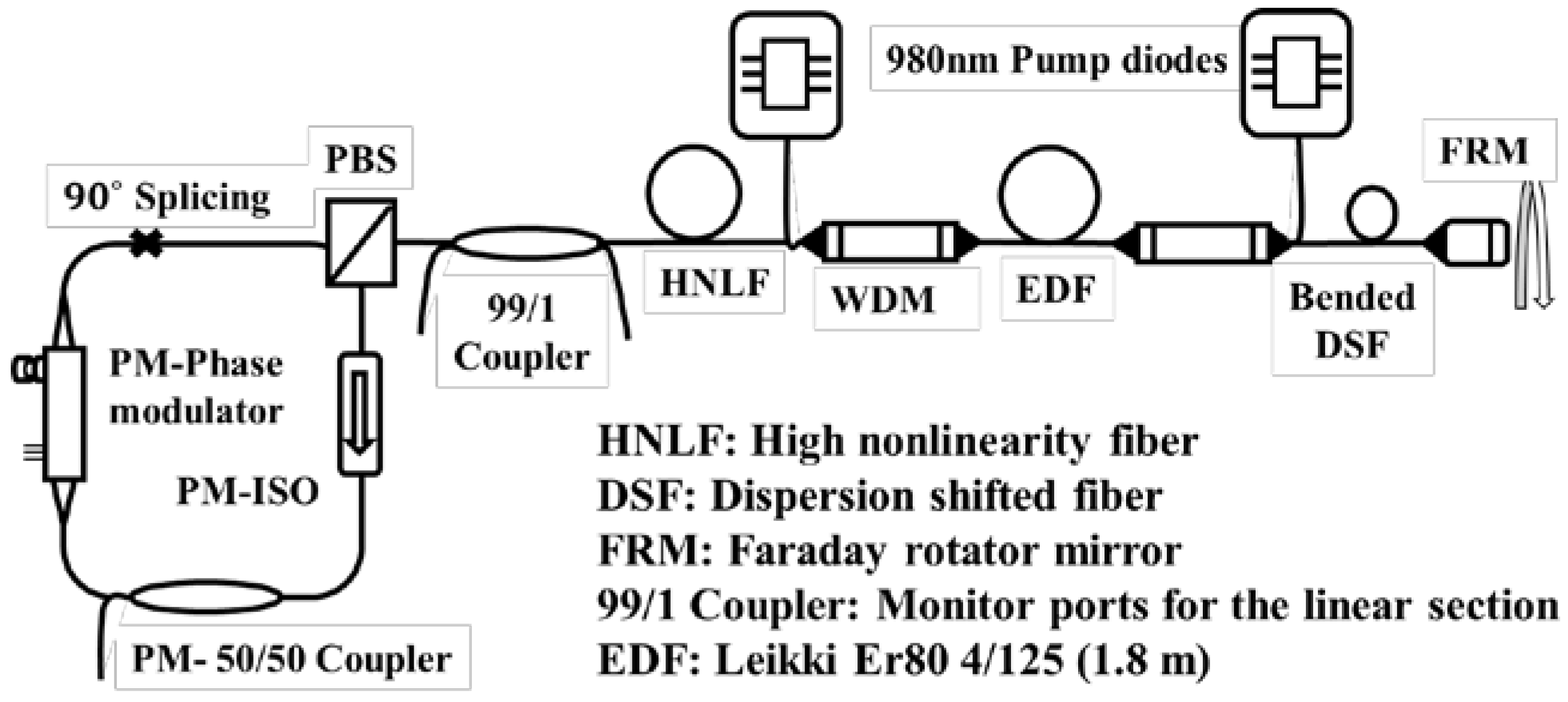
Our experimental mode-locked fiber laser configuration is constructed as a sigma-shape cavity which is able to achieve environmentally-stable operation, as indicated in Figure 1 [30,31,32,33,34]. The cavity is composed of a polarization-maintaining (PM) reflection loop, and a non-PM linear fiber section with a Farady rotator mirror for automatic birefringence cancellation. In the PM-loop, a LiNbO₃ phase modulator is inserted to provide an active mode-locking mechanism, and the phase modulation frequency is set at 10 GHz so that the laser can be harmonically mode-locked under a high repetition rate. In the non-PM linear section, a piece of 4 m dispersion-shifted high nonlinearity fiber (DS-HNLF) is used to enhance the cavity Kerr nonlinearity, and a piece of bent dispersion-shifted fiber (DSF) is inserted to adjust the lasing wavelength through its wavelength-dependent loss. The Er-doped gain laser is bi-directionally pumped so as to achieve enough lasing power for observing the bound-soliton mode-locking. Notice that in our mode-locked fiber laser, there is no equivalent saturable absorption effect [33,34]. The bound-soliton state can be formed in the higher pump power levels in comparison to the single-soliton state [25]. The RIN noises of both states are measured with a fast photo-detector and a radio frequency (RF) spectrum analyzer (Agilent E4440A, Santa Clara, CA, USA) for detailed comparison.

Our theoretical model is based on the Master equation, as shown in Equation (1), which assumes all the cavity parameters are averagely distributed. The physical meanings of the symbols are described as follow. $U\left(t,T\right)$: complex pulse envelope, $t$: small time scale, $T$: large time scale in terms of the cavity roundtrip number, $g_0$: small signal gain, $E_s$: gain saturation energy, $l_0$: linear loss, $d_i$: cavity dispersion, $d_r:$ optical filtering, $k_r$: equivalent nonlinear saturable absorption (=0 for the studied laser), $k_i$: self-phase modulation (SPM), $M:$ active phase modulation depth, $w_m$: modulation frequency, and $N\left(t,T\right)$: noise source.

$$\frac{\partial U}{\partial T}=\left(\frac{g_0}{1+\frac{{\displaystyle \int }{\left|U\right|}^{2}dt}{E_s}}-l_0\right)U+\left(d_r+j{d}_i\right)\frac{{\partial }^{2}U}{\partial t^2}+\left(k_r+j{k}_i\right)U^{*}UU+jMcos(w_{m}t)U+N\left(t,T\right)$$

(1)

The backpropagation method starts from the linearization of the above nonlinear equation. We assume a small perturbation field $u\left(t,T\right)$ around the mean field solution $u_0\left(t,T\right)$ and substitute $U\left(t,T\right)=u_0\left(t,T\right)+u\left(t,T\right)$ into Equation (1) to derive the linearized equation for $u\left(t,T\right)$. The result is shown in Equation (2).

$$\begin{array}{c}\frac{\partial u}{\partial T}=\left(\frac{g_0}{1+\frac{E_0}{E_s}}-l_0\right)u+\left(d_r+j{d}_i\right)\frac{{\partial }^{2}u}{\partial t^2}+\left(k_r+j{k}_i\right)\left(2u_0^{*}{u}_0\right)u+\left(k_r+j{k}_i\right)\left(u_0{u}_0\right)u^{*}\\ +jMcos\left(w_{m}t\right)u-\frac{g_0{u}_0}{{\left(1+\frac{E_0}{E_s}\right)}^2}\frac{1}{E_s}{\displaystyle \int }\left(u_0{u}^{*}+u_0^{*}u\right)dt+N\left(t,T\right)\end{array}$$

(2)

One can rewrite Equation (2) in a compact form, as in Equation (3). Note that the operator S now denotes a special operator that operates both on $u$ and $u^{*}$ as defined in Equation (2).

$$\frac{\partial u\left(t,T\right)}{\partial T}=S\left(t,T\right)·u\left(t,T\right)+N\left(t,T\right)$$

(3)

Corresponding to the above linearized perturbation equation, we then define an adjoint equation such that the inner-product conservation between two systems can be ensured. By introducing the adjoint operator of S according to the following Equation (4),

$$\langle u^A|S·u\rangle =\langle S^A·u^A|u\rangle$$

(4)

the adjoint equation is defined by Equation (5) as below:

$$\frac{\partial u^A\left(t,T\right)}{\partial T}=-S\left(t,T\right)·u^A\left(t,T\right)$$

(5)

Here, the inner product of two functions is defined as $\langle f\left(t\right)|g\left(t\right)\rangle =\frac{1}{2}{\displaystyle \int }\left(f{\left(t\right)}^{*}g\left(t\right)+f\left(t\right)g{\left(t\right)}^{*}\right)dt$. The complete form of the adjoint equation is given in Equation (6), where $E_0={\displaystyle \int }{u}_0^{*}{u}_{0}dt$ represents the mean field pulse energy.

$$\begin{array}{c}\frac{\partial u^A}{\partial T}=-\left(\frac{g_0}{1+\frac{E_0}{E_s}}-l_0\right)u^A-\left(d_r-j{d}_i\right)\frac{{\partial }^2{u}^A}{\partial t^2}-\left(k_r-j{k}_i\right)\left(2u_0^{*}{u}_0\right)u^A-\left(k_r+j{k}_i\right)\left(u_0{u}_0\right)u^{A^{*}}\\ +jMcos\left(w_{m}t\right)u^A+\frac{g_0{u}_0}{{\left(1+\frac{E_0}{E_s}\right)}^2}\frac{1}{E_s}{\displaystyle \int }\left(u_0{u}^{A^{*}}+u_0^{*}{u}^A\right)dt\end{array}$$

(6)

One can easily prove that the solutions of the linearized equation and its adjoint will satisfy:

$$\langle u^A\left(t,T\right)|u\left(t,T\right)\rangle =\langle u^A\left(t,0\right)|u\left(t,0\right)\rangle +{{\displaystyle \int }}_0^T\langle u^A\left(t,T^{\prime }\right)|N\left(t,T^{\prime }\right)\rangle d{T}^{\prime }$$

(7)

Equation (7) is main result of the backpropagation method, and is very physically meaningful. The final noise parameter defined by the projection in the left-hand side of Equation (7) comes from two contributions: the initial noise (the first term in the right-hand side) and the integrated added noises (the second term in the right-hand side). Thus, one can obtain information about the final noise parameter after numerically solving the adjoint system backwardly (from T to 0) with the initial condition given by $u^A\left(t,T\right)$, which is the projection function for the noise parameter to be analyzed. By choosing a suitable projection function, the inner product in the left-hand side of Equation (7) can correspond to the perturbation of the chosen pulse parameter. From the definition of the pulse energy $E={\displaystyle \int }{U}^{*}Udt$, for calculating the pulse energy noise of the optical pulse, the projection function is simply 2 times the mean field, as shown in Equation (8).

$$∆n\left(T\right)=\langle 2u_0\left(t,T\right)|u\left(t,T\right)\rangle$$

(8)

The noise variance $\mathrm{Var}\left[∆n\left(T\right)\right]$ and the noise auto-correlation function $\langle ∆n\left(T\right)∆n\left(T+∆T\right)\rangle$ can also be derived after knowing the statistical properties (i.e., white noises) of the noise source term $N\left(t,T\right)$. In the following, we will simply assume the noise is delta-function correlated, as given by Equation (9) [1,2,3,4], where $g=g_0/(1+\frac{E_0}{E_s})$ is the steady state gain coefficient of the laser and $\theta$ is the noise enhancement factor compared to the ideal quantum noise level.

$$\begin{array}{ll}\langle N^{*}\left(t_1,T_1\right)N\left(t_2,T_2\right)\rangle =& \langle N\left(t_1,T_1\right)N^{*}\left(t_2,T_2\right)\rangle =\theta *2gh\nu \delta \left(t_1-t_2\right)\delta \left(T_1-T_2\right)\\ & \langle N\left(t_1,T_1\right)N\left(t_2,T_2\right)\rangle =\langle N^{*}\left(t_1,T_1\right)N^{*}\left(t_2,T_2\right)\rangle =0\end{array}$$

(9)

The final formula for the intensity noise variance and the noise auto-correlation function are listed in Equations (10) and (11) below. Here we have assumed the contribution from the initial noise can be ignored, and only the integrated added noises are taken into account. For the mode-locked laser problems considered in the present work, this is a valid assumption.

$$\mathrm{Var}\left[∆n\left(T\right)\right]=\mathrm{Var}\left[{{\displaystyle \int }}_0^T\langle u^A\left(t,T^{\prime }\right)|N\left(t,T^{\prime }\right)\rangle d{T}^{\prime }\right]=\theta gh\nu {{\displaystyle \int }}_0^T{\displaystyle \int }Re[u^{A^{*}}\left(t,T\right)u^A\left(t,T\right)]dt dT$$

(10)

$$\begin{array}{ll}\langle ∆n\left(T+∆T\right)∆n\left(T\right)\rangle & =\langle {{\displaystyle \int }}_0^{T+∆T}\langle u_2^A\left(t^{″},T^{″}\right)|N\left(t^{″},T^{″}\right)\rangle d{T}^{″}{{\displaystyle \int }}_0^T\langle u_1^A\left(t^{\prime },T^{\prime }\right)|N\left(t^{\prime },T^{\prime }\right)\rangle d{T}^{\prime }\rangle \\ & =\theta gh\nu {{\displaystyle \int }}_0^T{\displaystyle \int }Re\left[u_2^{A^{*}}\left(t,T\right)u_1^A\left(t,T\right)\right]dt dT\end{array}$$

(11)

where in Equation (11), $u_1^A\left(t,T\right)$ and $u_2^A\left(t,T\right)$ are the two backpropagation solutions of the adjoint system corresponding to $∆n\left(T\right)$ and $∆n\left(T+∆T\right)$ respectively.

The general calculation procedures can be summarized in 3 steps. First of all, we forwardly propagate the nonlinear Equation (1) until the steady state of the mean field is reached. Secondly, we backwardly propagate the linear adjoint Equation (6) with the initial condition given by $2u_0\left(t,T\right)$ at the end point of the first step. Thirdly, we then utilize the Equations (10) and (11) to determine the noise variance and the noise auto-correlation function with the solution of the adjoint equation. The noise spectrum can then be computed by Fourier transforming the noise auto-correlation function [1,4]. The finite difference Crank-Nicholson method is used for propagating all the nonlinear and linearized equations. The whole calculation is deterministic, and thus, the required computation efforts are much reduced when compared to those required for the stochastic simulation method.

3. Results

The typical output characteristics of the experimental fiber laser are summarized in

Table 1. Main output characteristics of the fiber laser.

Operation States	Single Soliton	Bound Soliton
Output averaged power:	25 mW	55 mW
Pulse width/Timing distance	2.4 ps/X	1.95 ps/4.8 ps
Repetition rate	10 GHz
SMSR: (Super mode suppression)	50 dB under the REW 470 kHz

and illustrated in Figure 2. The laser can be operated under the single-soliton state at lower power levels, and under the bound-soliton state at higher power levels. In the middle of the transition, the laser is not very stable, mainly due to the co-existence of the two states. The measured pulse widths are in the ps level for both states, and the maximum output averaged power is near 60 mW. Figure 2a shows the auto-correlation trace for the single-soliton state. The red dashed line is the fitting curve with an assumed hyperbolic secant pulse shape. The insets of the sub-figures indicate the corresponding optical spectra. In the inset of Figure 2b, one can observe an interference dip located at the center of the spectrum, which indicates that the two bound-pulses are with π phase difference. Figure 2c,d show the RF spectral measurement results through a high speed photo-detector for both the single- and bound-soliton states. The repetition rate is around 10 GHz and the laser is with a good super mode suppression ratio (SMSR).

Figure 3 shows the measurement data for the laser intensity noise spectra with a span from 1 kHz to 500 kHz, and a resolution bandwidth of 10 Hz. In the measurement range from 1 kHz to 500 kHz, one can avoid the dominant pump-induced amplitude noises near direct current (DC) so as to more clearly observe the intrinsic pulse intensity fluctuations of the mode-locked fiber laser [13,14,15]. The measurement results approach the background floor at frequencies higher than 500 kHz. One can observe a flat intensity noise spectrum for both states from 1 kHz to the turning point near 100 kHz. The noise of the bound-soliton state is lower than that of the single-soliton state. The averaged noise power levels for the single- and bound- soliton states within the span from 1 kHz to 30 kHz are −96 dBm and −101 dBm respectively, and the total integrated power within the span from 1 kHz to 500 kHz are −36.3 dBm and −38.3 dBm. One can observe some oscillation peaks near the turning point for both states, and the flat bandwidth of the bound-soliton state is wider than that of the single-soliton state. One possible cause for these peaks is the relaxation oscillation effect caused by the gain dynamics inside the cavity [6,35]. However, as we will see in the theoretical results below, parts of these resonance peaks may also be attributed to the mode-locking dynamics. Note that, experimentally, we cannot operate the single- and bound-soliton states under the same power level, because the laser becomes unstable due to the co-existence of the two states. Therefore, for direct experimental comparison, the measurement results for both states are performed with the same averaged optical power incident on the photo-detector through the use of an optical attenuator.

For numerically calculating the intensity noises, the physical normalization units and the various cavity parameters used in our simulation are given below. The normalization unit of $t$ is 0.5 ps, and the unit of $T$ is the cavity roundtrip time, which is about 200 ns, as determined from the cavity length. The normalization unit of the pule energy is 10 pJ, which is estimated from the experimental results. The group velocity dispersion parameter $d_i=0.4$ is estimated from the experimental condition. We set the SPM parameter at $k_i=0.7$ according to the soliton assumption, and finely adjust it to make the numerical and experimental results better matched. The saturable absorption parameter $k_r$ is set to 0 because there was no passive saturable absorption in our laser due to the sigma-type cavity. The phase modulation frequency is set around 10 GHz, with a modulation depth around 1. The cavity linear gain is set to be variable from $g_0$ = 2.5 to 5 to accord with the lower and higher power level cases according to the relation ${\displaystyle \int }{\left|u_0\right|}^{2}dt\approx \left(g_0/l_0-1\right)E_s$ [25]. The noise enhancement factor $\theta$ is set to be 10. Other parameters are also reasonably determined so that the simulation results can be closely matched with the experimental results. The initial condition of the single-soliton case is a symmetrically single secant-shape pulse, and the initial condition of the bound-soliton case is two anti-symmetrical secant-shape pulses with $\mathsf{\pi }$ phase difference. The total propagation distance in the simulation is 1000 roundtrips with the step size dT = 0.005. The small-scale time step is dt = 0.01 in the normalization units, and the total simulation window is 25 ps. We have checked that these step sizes are small enough to ensure the accuracy of the calculation.

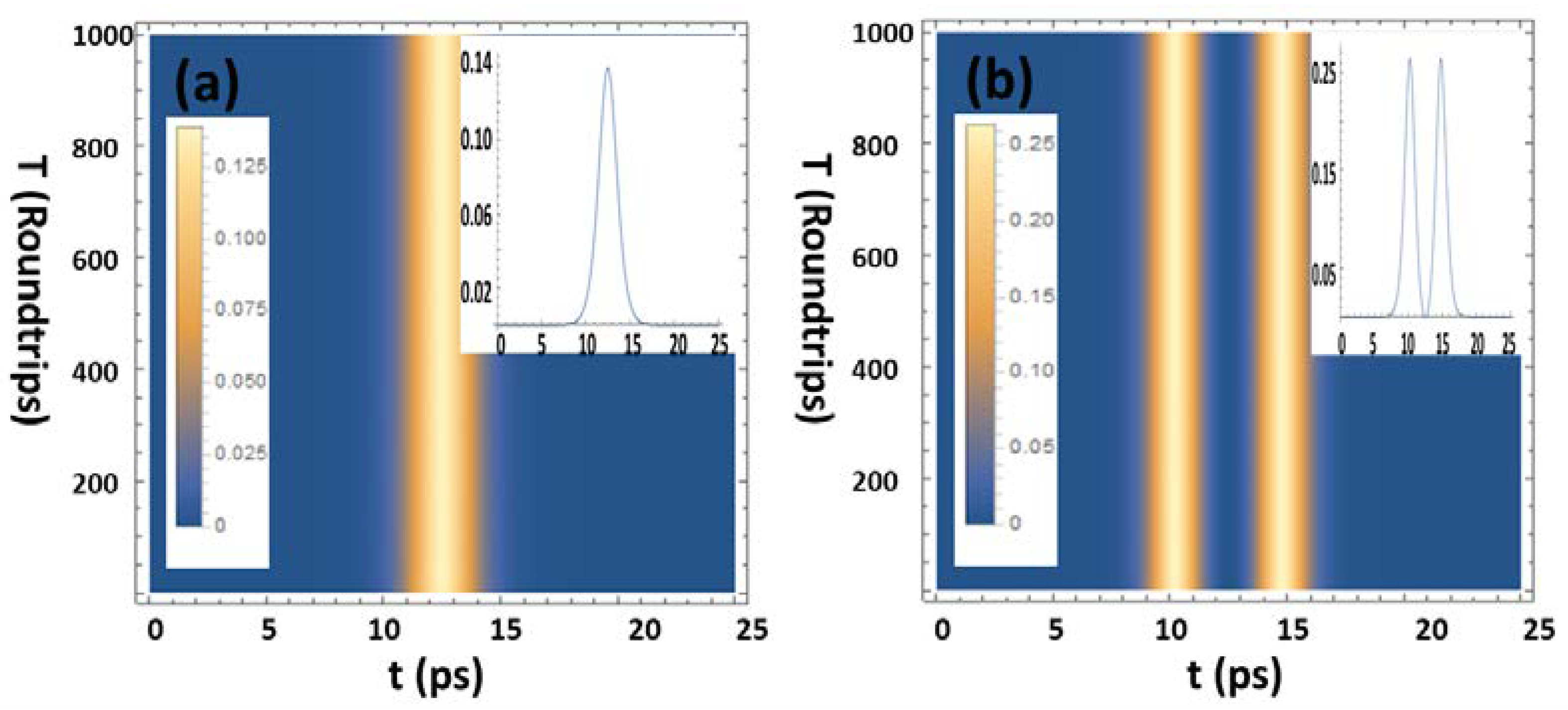
Figure 4 shows the steady state propagation solutions of the single- and bound-soliton states in the case of $g_0$ = 2.5 and 5. The pulse width for the single-soliton is around 2.41 ps, while the pulse width and timing separation of the bound-soliton state are around 1.72 and 4.58 ps. We gradually increase $g_0$ from 2.5 to 5 to investigate the pulse properties under different pulse energies. Figure 5a indicates the simulated pulse energy for both states versus $g_0$. Basically, a linear relation can be obtained to match with the relation ${\displaystyle \int }{\left|u\right|}^{2}dt\approx \left(g_0/l_0-1\right)E_s$. Figure 5b is the pulse width and bound-pulse timing separation as a function of $g_0$. The pulse width and timing separation are both decreased when $g_0$ is increased, because of larger nonlinearity. The pulse width reduction is extremely sensitive in the single-soliton state; this is because the single-soliton is with a larger peak power to induce larger nonlinearity. Figure 5c shows the required steady-state lasing gain for the considered mode-locking states by analyzing the Master equation as an eigenvalue problem [25,36]. The negative real part of the solved eigenvalue exactly corresponds to the required steady-state lasing gain for the corresponding mode-locking state in the presence of all the cavity effects. Physically, the state with the minimum steady-state lasing gain is the most stable solution that will emerge as the final steady state of the system. This is because once the state emerges, other states will see net losses, and thus, decay away. This is why the steady state lasing gain can be used as a meaningful physical quantity for determining the stability of the lasing states. Nevertheless, if there are several states with enough close steady-state lasing gains, the perturbations in the laser can cause state jumping, and the differential losses may be too small to make the perturbations decay quickly. Under this situation the laser will become unstable. One can see that the required steady state lasing gains for the single- and bound-soliton states are very close in the overlap region marked by the blue circle. The laser operation within this region is expected to be not very stable experimentally, due to the co-existence of two states with close steady state lasing gains, since small fluctuations of the laser will easily lead to state jumping under this condition. This explains why, experimentally, we can only operate the laser under the single-soliton state in the lower power level, and under the bound-soliton state in the higher power level.

Figure 6a,b are the theoretical single sideband RIN spectra, derived by taking the Fourier transform of the noise auto-correlation functions calculated by the linearized backpropagation method for both the single- and bound-soliton states respectively. The main difference of the noise spectra between the two states is the level of the flat spectral distribution from 1 kHz to the turning point near 100 kHz. The bound-soliton state has a lower noise level, which is in good agreement with the observed experimental tendency. Moreover, the flat bandwidth of the bound-soliton state is wider than that of the single-soliton state, i.e., about tens of kHz. This again agrees with the experiment. Some resonance peaks can also be resolved near the turning point for both states, which can be attributed to the coupling effects of different pulse parameters [4]. Since the relaxation oscillation effects of the Er-doped fiber lasers may also show up in this range of frequencies, one may not be able to resolve these resonance peaks experimentally. Figure 6c shows the integrated noise variance within the span from 1 kHz to 2.5 MHz versus different values of $g_0$. The integrated RIN noise variance for the single- and bound-soliton states are $7.56\times {10}^{-7}$ and $2.69\times {10}^{-7}$ at $g_0$ = 2.5 and $g_0$ = 5 respectively, which corresponds to the energy fluctuations of 0.087% and 0.052% respectively. Both the single- and bound-soliton RIN variances decrease when the pulse energy gets larger. The bound-soliton states have smaller RIN noises compared to the single-soliton states of the same laser by following the similar lasing power scaling tendency as shown in Figure 6c.

4. Discussion

In the present work, the RIN noise modelling as well as the RIN spectrum calculation for bound-pulse mode-locked lasers are theoretically investigated by the linearized backpropagation method for the first time. The developed general method can provide an efficient way to calculate the mode-locked laser noises without the need of assuming a particular optical pulse shape, which enable us to deal with more general laser noise problems. As an example, the intensity noise properties of an environmentally-stable hybrid mode-locked Er-doped fiber laser are studied both experimentally and theoretically. The laser can be operated at a 10 GHz repetition rate, with either the single- or bound-soliton output, depending on the lasing power level. With this unique laser setup, we are able to compare the RIN noises of the single- or bound-soliton mode-locking states more precisely. The theoretical calculation predicts that the RIN noises for the bound-soliton states can be few dB lower than the RIN noises for the single-soliton states of the same laser. The experimental measurements confirm this prediction, even though currently, the noise reduction factor is not very large. The results suggest the new possibility of generating high repetition rate optical bound-pulses with lower relative intensity noises, and also demonstrate that the developed theoretical modelling based on the linearized backpropagation approach is a very powerful method for studying general mode-locked laser noise problems.

References

- Haus, H.A.; Mecozzi, A. Noise of Mode-Locked Lasers. IEEE J. Quantum Electron. 1993, 29, 983–996. [Google Scholar] [CrossRef]
- Yu, C.X.; Namiki, S.; Haus, H.A. Noise of the Stretched Pulse Fiber Laser: Part II—Experiments. IEEE J. Quantum Electron. 1997, 33, 660–668. [Google Scholar] [CrossRef]
- Grein, M.E.; Jiang, L.A.; Haus, H.A.; Ippen, E.P.; McNeilage, C.; Searls, J.H.; Windeler, R.S. Observation of quantum-limited timing jitter in an active, harmonically mode-locked fiber laser. Opt. Lett. 2002, 27, 957–959. [Google Scholar] [CrossRef] [PubMed]
- Grein, M.E.; Haus, H.A.; Chen, Y.; Ippen, E.P. Quantum-Limited Timing Jitter in Actively Modelocked Lasers. IEEE J. Quantum Electron. 2004, 40, 1458–1470. [Google Scholar] [CrossRef]
- Yoshida, E.; Nakazawa, M. Measurement of the Timing Jitter and Pulse Energy Fluctuation of a PLL Regeneratively Mode-Locked Fiber Laser. IEEE Photonics Technol. Lett. 1999, 11, 548–550. [Google Scholar] [CrossRef]
- Paschotta, R. Noise of mode-locked lasers (Part II): Timing jitter and other fluctuations. Appl. Phys. B 2004, 79, 163–173. [Google Scholar] [CrossRef]
- Kim, J.; Chen, J.; Cox, J.; Kärtner, F.X. Attosecond-resolution timing jitter characterization of free-running mode-locked lasers. Opt. Lett. 2007, 32, 3519–3521. [Google Scholar] [CrossRef] [PubMed]
- Song, Y.; Kim, C.; Jung, K.; Kim, H.; Kim, J. Timing jitter optimization of mode-locked Yb-fiber lasers toward the attosecond regime. Opt. Express 2011, 19, 14518–14525. [Google Scholar] [CrossRef] [PubMed]
- Shin, J.; Jung, K.; Song, Y.; Kim, J. Characterization and analysis of timing jitter in normal-dispersion mode-locked Er-fiber lasers with intra-cavity filtering. Opt. Express 2015, 23, 22898–22906. [Google Scholar] [CrossRef] [PubMed]
- Tamura, K.; Nakazawa, M. Timing jitter of solitons compressed in dispersion-decreasing fibers. Opt. Lett. 1998, 23, 1360–1362. [Google Scholar] [CrossRef] [PubMed]
- Chen, W.; Song, Y.; Jung, K.; Hu, M.; Wang, C.; Kim, J. Few-femtosecond timing jitter from a picosecond all-polarization-maintaining Yb-fiber laser. Opt. Express 2016, 24, 1347–1357. [Google Scholar] [CrossRef] [PubMed]
- Menyuk, C.R.; Wang, S. Spectral Methods for Determining the Stability and Noise Performance of Passively Modelocked Lasers. Nanophotonics 2016, 5, 332–350. [Google Scholar] [CrossRef]
- Budunoğlu, I.L.; Ülgüdür, C.; Oktem, B.; Ilday, F.Ö. Intensity noise of mode-locked fiber lasers. Opt. Lett. 2009, 34, 2516–2518. [Google Scholar] [CrossRef] [PubMed]
- Wu, K.; Shum, P.P.; Aditya, S.; Ouyang, C.; Wong, J.H.; Lam, H.Q.; Lee, K.E.K. Noise conversion from pump to the passively mode-locked fiber lasers at 1.5 μm. Opt. Lett. 2012, 37, 1901–1903. [Google Scholar] [CrossRef] [PubMed]
- Chen, J.; Sickler, J.W.; Ippen, E.P.; Kärtner, F.X. High repetition rate, low jitter, low intensity noise, fundamentally mode-locked 167 fs soliton Er-fiber laser. Opt. Lett. 2007, 32, 1566–1568. [Google Scholar] [CrossRef] [PubMed]
- Kim, C.; Jung, K.; Kieu, K.; Kim, J. Low timing jitter and intensity noise from a soliton Er-fiber laser mode-locked by a fiber taper carbon nanotube saturable absorber. Opt. Express 2012, 20, 29524–29530. [Google Scholar] [CrossRef] [PubMed]
- Kim, D.; Zhang, S.; Kwon, D.; Liao, R.; Cui, Y.; Zhang, Z.; Song, Y.; Kim, J. Intensity noise suppression in mode-locked fiber lasers by double optical bandpass filtering. Opt. Lett. 2017, 42, 4095–4098. [Google Scholar] [CrossRef] [PubMed]
- Tang, D.Y.; Zhao, B.; Shen, D.Y.; Lu, C.; Man, W.S.; Tam, H.Y. Bound-soliton fiber laser. Phys. Rev. A 2002, 66, 033806. [Google Scholar] [CrossRef] [Green Version]
- Tang, D.Y.; Zhao, B.; Zhao, L.M.; Tam, H.Y. Soliton interaction in a fiber ring laser. Phys. Rev. E 2005, 72, 016616. [Google Scholar] [CrossRef] [PubMed] [Green Version]
- Wu, X.; Tang, D.Y.; Luan, X.N.; Zhang, Q. Bound states of solitons in a fiber laser mode locked with carbon nanotube saturable absorber. Opt. Commun. 2011, 284, 3615–3618. [Google Scholar] [CrossRef]
- Yun, L.; Liu, X. Generation and propagation of bound-state pulses in a passively mode-locked figure-eight laser. IEEE Photonics J. 2012, 4, 512–519. [Google Scholar]
- Wang, Z.; Zhan, L.; Majeed, A.; Zou, Z. Harmonic mode locking of bound solitons. Opt. Lett. 2015, 40, 1065–1068. [Google Scholar] [CrossRef] [PubMed]
- Hsiang, W.W.; Lin, C.Y.; Lai, Y. Stable new bound soliton pairs in a 10 GHz hybrid frequency modulation mode-locked Er-fiber laser. Opt. Lett. 2006, 31, 1627–1629. [Google Scholar] [CrossRef] [PubMed]
- Nguyen, N.D.; Binh, L.N. Generation of high order multi-bound solitons and propagation in optical fibers. Opt. Commun. 2009, 282, 2394–2406. [Google Scholar] [CrossRef]
- Luo, C.J.; Wang, S.M.; Lai, Y. Bound Soliton Fiber Laser Mode-Locking Without Saturable Absorption Effect. IEEE Photonics J. 2016, 8, 1502609. [Google Scholar] [CrossRef]
- Luo, C.J.; Lai, Y. RIN noise reduction effect of a 10 GHz hybrid bound soliton mode-locked fiber laser. In Proceedings of the IEEE Photonics Conference, Waikoloa, HI, USA, 2–6 October 2016. [Google Scholar]
- Lai, Y.; Yu, S.S. General quantum theory of nonlinear optical-pulse propagation. Phys. Rev. A 1995, 51, 817–829. [Google Scholar] [CrossRef] [PubMed]
- Lee, R.K.; Lai, Y.; Malomed, B.A. Quantum correlations in bound-soliton pairs and trains in fiber lasers. Phys. Rev. A 2004, 70, 063817. [Google Scholar] [CrossRef] [Green Version]
- Lee, R.K.; Lai, Y.; Malomed, B.A. Photon-number fluctuation and correlation of bound soliton pairs in mode-locked fiber lasers. Opt. Lett. 2005, 30, 3084–3086. [Google Scholar] [CrossRef] [PubMed]
- Yamashita, S.; Hotate, K.; Ito, M. Polarization properties of a reflective fiber amplifier employing a circulator and a Faraday rotator mirror. J. Lightwave Technol. 1996, 14, 385–390. [Google Scholar] [CrossRef]
- Carruthers, T.F.; Duling, I.N., III. 10-GHz, 1.3-ps erbium fiber laser employing soliton pulse shortening. Opt. Lett. 1996, 21, 1927–1929. [Google Scholar] [CrossRef] [PubMed]
- Carruthers, T.F.; Duling, I.N., III; Horowitz, M.; Menyuk, C.R. Dispersion management in a harmonically mode-locked fiber soliton laser. Opt. Lett. 2000, 25, 153–155. [Google Scholar] [CrossRef] [PubMed]
- Jones, D.J.; Nelson, L.E.; Haus, H.A.; Ippen, E.P. Diode-pumped environmentally stable stretched-pulse fiber laser. IEEE J. Sel. Top. Quantum Electron. 1997, 3, 1076–1079. [Google Scholar] [CrossRef]
- Carruthers, T.F.; Duling, I.N., III; Dennis, M.L. Active-passive modelocking in a single-polarisation erbium fibre laser. Electron. Lett. 1994, 30, 1051–1053. [Google Scholar] [CrossRef]
- Yang, S.; Ponomarev, E.A.; Bao, X. Experimental study on relaxation oscillation in a detuned FM harmonic mode-locked Er-doped fiber laser. Opt. Commun. 2005, 245, 371–376. [Google Scholar] [CrossRef]
- Wu, S.Y.; Hsiang, W.W.; Lai, Y. Synchronous-asynchronous laser mode-locking transition. Phys. Rev. A 2015, 92, 013848. [Google Scholar] [CrossRef]
Figure 1.
Configuration of the environmentally stable 10 GHz hybrid mode-locked Er-doped fiber laser with a sigma-type fiber cavity.
Figure 2.
Auto-correlation and optical spectrum measurements for (a) single- and (b) bound-soliton states respectively. The red dashed line in (a) shows the pulse intensity auto-correlation fitting under the sech shape assumption. RF spectrum measurement for (c) single- and (d) bound-soliton states within the 50 MHz span range with the resolution bandwidth of 470 kHz.
Figure 3.
Measured intensity fluctuations of (a) single-soliton state with output averaged power of 25 mW; (b) bound-soliton state with output averaged power of 55 mW. The span range is from 1 kHz to 500 kHz. For direct comparison, the measurement results for both states are performed with the same averaged optical power incident on the photo-detector through the use of an optical attenuator.
Figure 4.
Numerical simulation results for (a) single-soliton case at g0 = 2.5; (b) bound-soliton case at g0 = 5, both within 1000 roundtrips propagation.
Figure 5.
Numerical simulation results of (a) pulse energy; (b) pulse width and bound-pulse timing distance and (c) required lasing gain versus g0 for the single- and bound-soliton states respectively.
Figure 6.
The calculated RIN spectra for (a) single-soliton state at = 2.5 and (b) bound-soliton state at = 5 within the span from 1 kHz to 2.5 MHz. (c) The integrated intensity noise variance versus within the same span.