Measurements of High-Frequency Atmospheric Turbulence and Its Impact on the Boundary Layer of Wind Turbine Blades


Mechanical Engineering Department, Kiel University of Applied Sciences, D-24149 Kiel, Germany
*
Author to whom correspondence should be addressed.
Appl. Sci. 2018, 8(9), 1417; https://doi.org/10.3390/app8091417
Submission received: 12 June 2018
/
Revised: 24 July 2018
/
Accepted: 8 August 2018
/
Published: 21 August 2018
(This article belongs to the Special Issue Wind Turbine Aerodynamics)
Abstract
:To gain insight into the differences between onshore and offshore atmospheric turbulence, pressure fluctuations were measured for offshore wind under different environmental conditions. A durable piezo-electric sensor was used to sample turbulent pressure data at 50 kHz. Offshore measurements were performed at a height of 100 m on Germany’s FINO3 offshore platform in the German Bight together with additional meteorological data provided by Deutscher Wetterdienst (DWD). The statistical evaluation revealed that the stability state in the atmospheric boundary does not seem to depend on simple properties like the Reynolds number, wind speed, wind direction, or turbulence level. Therefore, we used higher statistical properties (described by so-called shape factors) to relate them to the stability state. Data was classified to be either within an unstable, neutral, or stable stratification. We found that, in case of stable stratification, the shape factor was mostly close to zero, indicating that a thermally stable environment produces closer-to Gaussian distributions. Non-Gaussian distributions were found in unstable and neutral boundary layer states, and an occurrence probability was estimated. Possible impacts on the laminar-turbulent transition on the blade are discussed with the application of so-called laminar airfoils on wind turbine blades.
1. Introduction
The use of wind energy has been very successful during the last decades [1], reaching a nearly stable annual investment corresponding to 50 GW of rated power word-wide. This was in connection and in parallel to an impressive development in Wind Turbine Aerodynamics [2] and even a special branch of wind energy meteorology has been established [3].
Due to the increased number of annual new installations, site assessment for wind farms has become more and more important and sophisticated, even under offshore conditions, with application to tailored turbine design as well. For a selection of important references on properties of the atmospheric boundary layer on- and off-shore see, for example, reference [4,5,6,7]. In most cases, turbulence has been treated in the context of loads, and frequency ranges higher than a few Hertz have generally been considered to be of no importance. However, this high frequency turbulence plays a significant role in laminar-to-turbulent transition inside the boundary layer of blades for airplanes [8,9] and wind turbines [10,11]. Due to the much higher drag of turbulent parts, this may give rise lower wind turbine efficiency (in terms of , the number measures the fraction of extracted power from the wind) as desired, and the proper choice of airfoils is crucial.
In this paper, these high-frequency turbulent statistics were studied with respect to higher order statistical moments in some detail using the method of super-statistics [12]. The shape factor from reference [13]—which gives estimates of the extent to which turbulent fluctuations diverge from Gaussian behavior—was of special interest.
Unlike earlier investigations, the non-Gaussianity of turbulent pressure fluctuations could not be linked to one of the more popular atmospheric parameters like the Reynolds number based on Taylor’s micro-scale [14], wind speed, or others. Therefore, we propose characterizing our findings according to the stability of the atmospheric boundary layer in terms of Richardson’s number. This paper is organized as follows: Firstly, the measurement setup is described together with the locations at which they were performed. Then, we describe the procedure of data analysis. After that, we present and discuss our findings and finally, draw some conclusions.
Parts of the material have been presented earlier in unpublished proceedings of ICOWES2013 [15].
2. Measurements
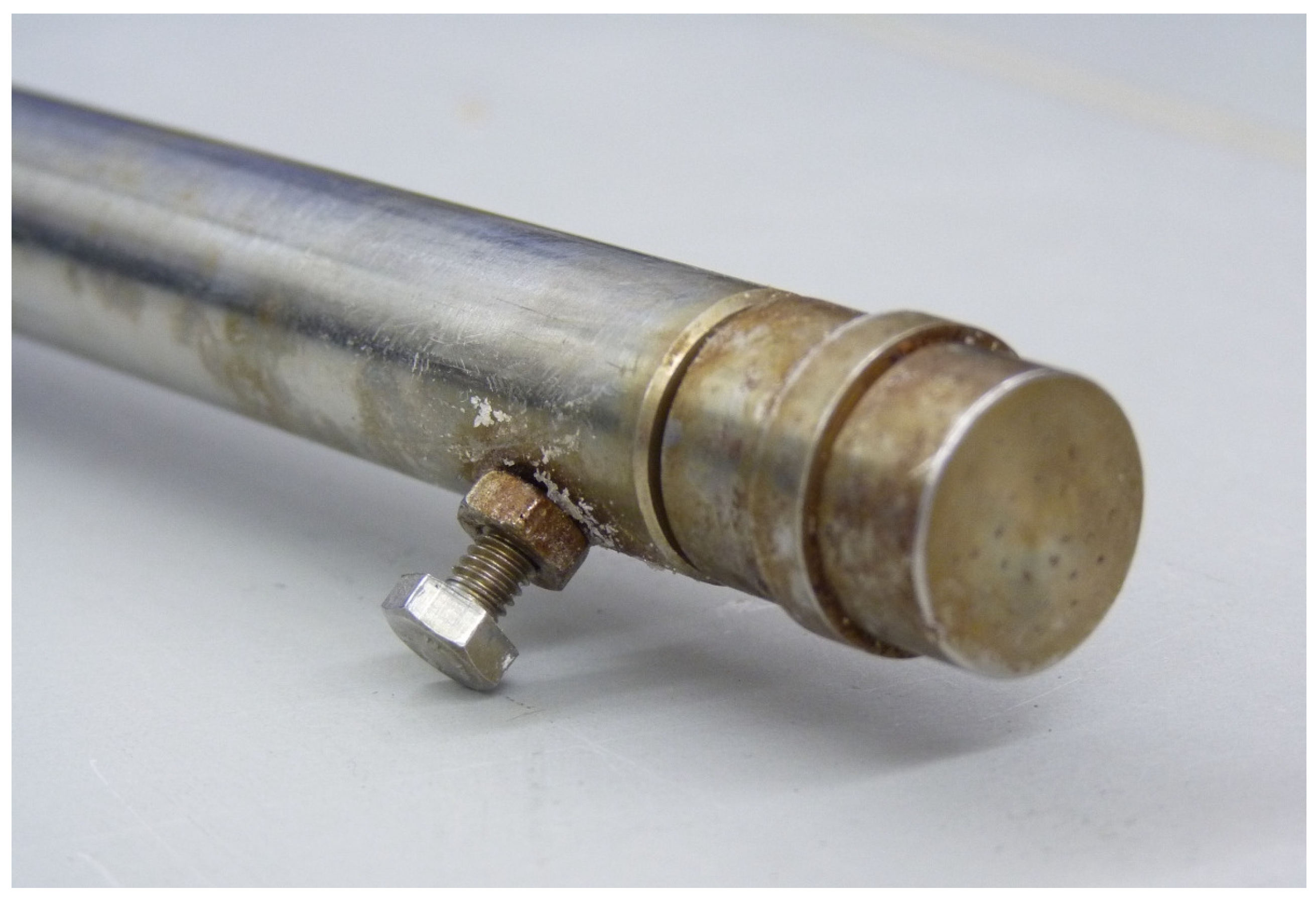
Our first set of high-resolution measurements (during the years 2009 until 2011) was performed using piezoelectric pressure sensors from PCB Piezotronics (Figure 1) that were connected to an imc Meßsystem GmbH CS-1208 data logger. The diameter of the sensing element was 15 mm. The minimal pressure resolution was 0.13 Pa, and the possible temporal resolution ranged from 2.5 Hz to 80,000 Hz.
Reference [16] discusses how the length, which is usually more than 100 times larger than the diameter of a hot-wire, influences the spatially resolution.
In our measurements, the pressure data was sampled at 50 kHz with a total duration of 100 s. The wind speed and temperature were sampled with a 1 Hz temporal resolution.
The piezoelectric pressure sensor was calibrated against a hot wire anemometer in a wind tunnel at the University of Oldenburg. The turbulent wind speed from the hot wire anemometer and the variation in turbulent pressure showed the same statistical properties up to 3 kHz (see [17]).
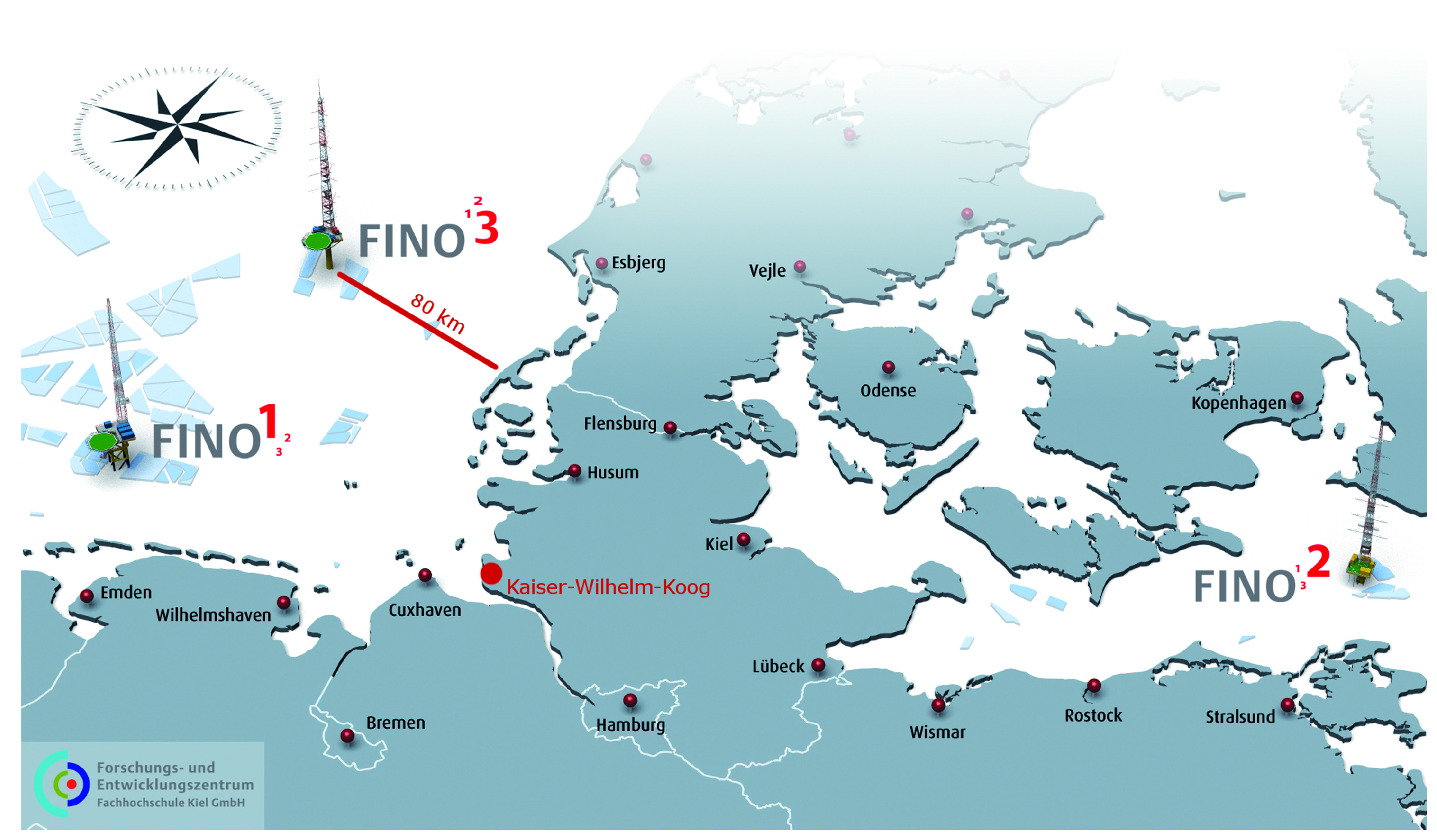
Onshore measurements were conducted at the Kaiser–Wilhelm–Koog test site of Germanischer Lloyd/Garrad Hassan (see Figure 2). A lattice tower of 60 m height provided booms to mount the pressure sensor on and other measurement equipment. The pressure sensor was mounted at a height of 55 m. The wind speed and wind direction were recorded at a height of 55 m by calibrated cup anemometers and wind vanes, respectively. The temperature was recorded at height of 53 m by a resistor-type thermometer.
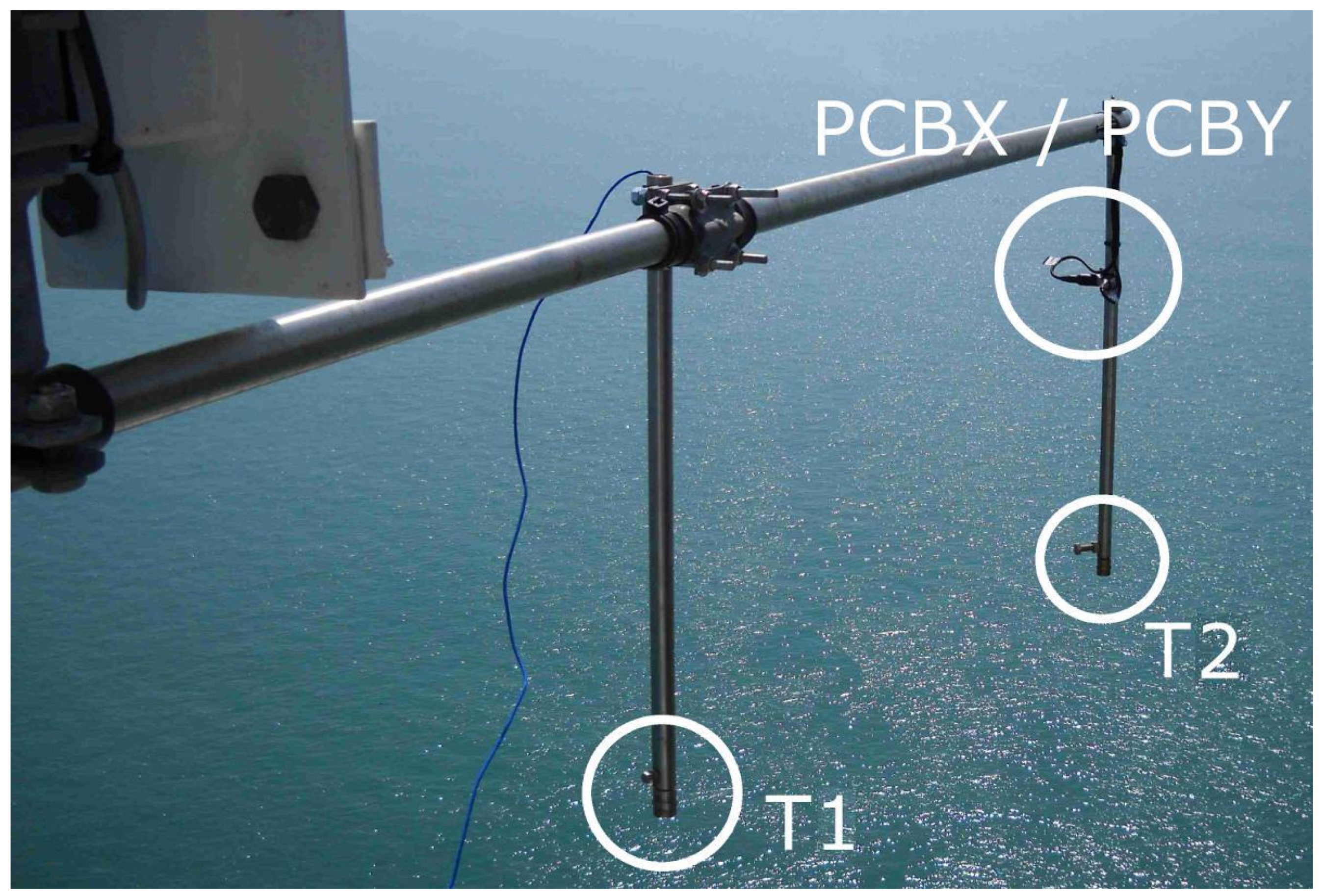
FEZ Kiel’s platform FINO3 was the location for the offshore measurements. About 80 km west of the island of Sylt (see Figure 2) the platform was constructed close to (at that time not) operational wind farms like DanTysk and Sandbank 24. The tower is a lattice tower type with booms of sufficient length for undisturbed measurements. Two pressure sensors (Figure 3) were mounted at a height of about 100 m above the mean sea level for parallel operation. The data acquisition equipment for meteorological signals was similar to that used onshore. The wind speed and wind direction were measured at a height of 100 m, and the temperature was measured at a height of 95 m above the mean sea level.
3. Analysis
Our recorded data sets were put into wind speed classes starting at 6 m/s, 12 m/s, and 16 m/s. Measurements were triggered manually if wind conditions were regarded as suitable. The bin size for each class was generally ±2 m/s, and for some cases (offshore class 10 m/s, offshore class 12 m/s), it was less (lower limit: −1 m/s). For each measurement, the statistical characteristics were analyzed with respect to the power-spectral density, incremental distributions, shape factors, structure functions, auto-correlations and Taylor’s micro-scale. (It may be interesting to note that Taylor’s micro-scale may have an complementary interpretation to the Markov–Einstein coherence length [18]. To use this one seems to be much more physical than the somewhat vague interpretation of the average turbulent vortex size.) We now explain our methods in more detail.
The increments of measured quantities were defined as
where u is the velocity, p is the pressure, t is the time, and is a fixed time increment. The increments also eliminated the mean value of the time series and thus, stochastic fluctuations remained for a specific time scale (). These increments were the basic statistical quantities used for more sophisticated analyses like structure functions or the so-called shape parameter. Reference [13] suggested that the distribution of increments may be described as a superposition of two distributions, one of them being lognormal. The shape factor then may be regarded as a measure of the level of intermittency. In accordance with Beck’s approach from reference [12], the shape parameter can be calculated by the 2nd and 4th order moments of the distribution:
where is the shape factor for the velocity and is the shape factor for the pressure. The brackets define the mean value of a quantity (x). Further properties are given in reference [12]. A value of indicates a normal distribution. It is worth noting that another important parameter for the deviation from Gaussian behavior, skewness, which is related to third-order moments, was found to be small [17].
It has well-known, at least since the work of reference [19], that turbulent velocities and pressures obey different scaling laws ( and , respectively), although they are seemingly related by according to Bernoulli’s law. A direct comparison of a hot-wire with piezo-electric pressure sensor data showed comparable power density spectra up to 4 kHz (see [17], unpublished), however. Theoretical as well as experimental investigations of reference [20] are still incomplete, so that there is no clear answer so far about how and are related to each other.
When heat transfer occurs, such as in the atmospheric boundary layer if the sea is warmer than the air (autumn), thermal stratification becomes more important. Simple static stability of the boundary layer may be used to characterize levels of turbulence. As was shown by reference [21], the turbulence intensity differs remarkably for stable and unstable flow when used to describe fatigue loads of wind turbines.
A simple characterization of a stratified boundary layer exposed to heat transfer was introduced by reference [4] as being stable, neutral, or unstable. Different calculation methods have been used to distinguish these states ([4]) depending on what is known in terms of input. In our case, a Richardson’s number approach was used, in accordance with common practice in wind energy meteorology [22,23,24].
This was defined as
where g is the acceleration of gravity, T is the mean absolute temperature, z is the height normal to the surface, and is the mean velocity the gradient. The z-direction was assumed to be vertical. The potential temperature () is defined as
where p is the pressure, and hPa is the reference pressure, is the specific gas constant, and is the specific heat capacity of air. It has to be noted that we checked for the influence of humidity and found that the influence on density as well as specific humidity [5] was below 1%. We therefore neglected all moisture corrections to Richardson’s Number (Ri).
In Equation (3), the quantity describes the forces introduced by heat transfer in the boundary layer. The term represents the momentum forces in the boundary layer. If we consider two points in the boundary layer at heights and where and , from (3) can be rewritten with the differences between the two locations as
We always assumed the presence of positive velocity gradients so only the convective part of Equation (5) remained. Three typical situations were then distinguished as follows:
- The surface is colder than the fluid and the gradient becomes and therefore, . Heat is transported by conduction only, and a convection flow does not occur. In this case, the stratification is strong, and turbulence gets damped. The boundary condition is stable for .
- The temperature gradient is zero and therefore, . There is no temperature gradient and therefore, no conduction nor convection. This condition is called neutral.
- The surface is warmer than the fluid and the gradient becomes and therefore, . Heat is transported by conduction and by convection from the surface to the fluid. The convection results in a vertical, upward component of the flow that interacts with the horizontal velocity component. This leads to the production of turbulence in the boundary layer and therefore, is called unstable.
From our measurements we obtained the necessary values for p, at a height of 100 m , wind speed , and wind direction as well as the sensor signal of the piezoelectric microphone. By assuming the air was a perfect gas, the density was calculated by the perfect gas law.
For the derivatives and , the temperature and wind speed at a second height needed to be known. Unfortunately, these data were not available during most of our measurements. Therefore, these gradients had to be approximated in a different way.
The ground temperature () was estimated using data from the Deutscher Wetterdienst (DWD). For the onshore measurements, the ground temperature at a nearby location was available at hourly samples. The temperature of the sea for the offshore measurements was interpolated from measurement stations on the island of Helgoland and at List on the island of Sylt.
The sign of mostly depends on the temperature gradient, so the velocity gradient can be regarded as of lower importance. Therefore, as a rough estimate, was used to calculate the velocity gradient. This mostly affected the absolute value of but not the heat transfer conditions in the atmospheric boundary layer.
With this procedure, estimates for were possible. The identification of stable or unstable states was simple. However, the neutral state required a value of exactly which was difficult to attain precisely within our set of approximations. To indicate a nearly neutral state, a bandwidth of was used instead.
4. Results
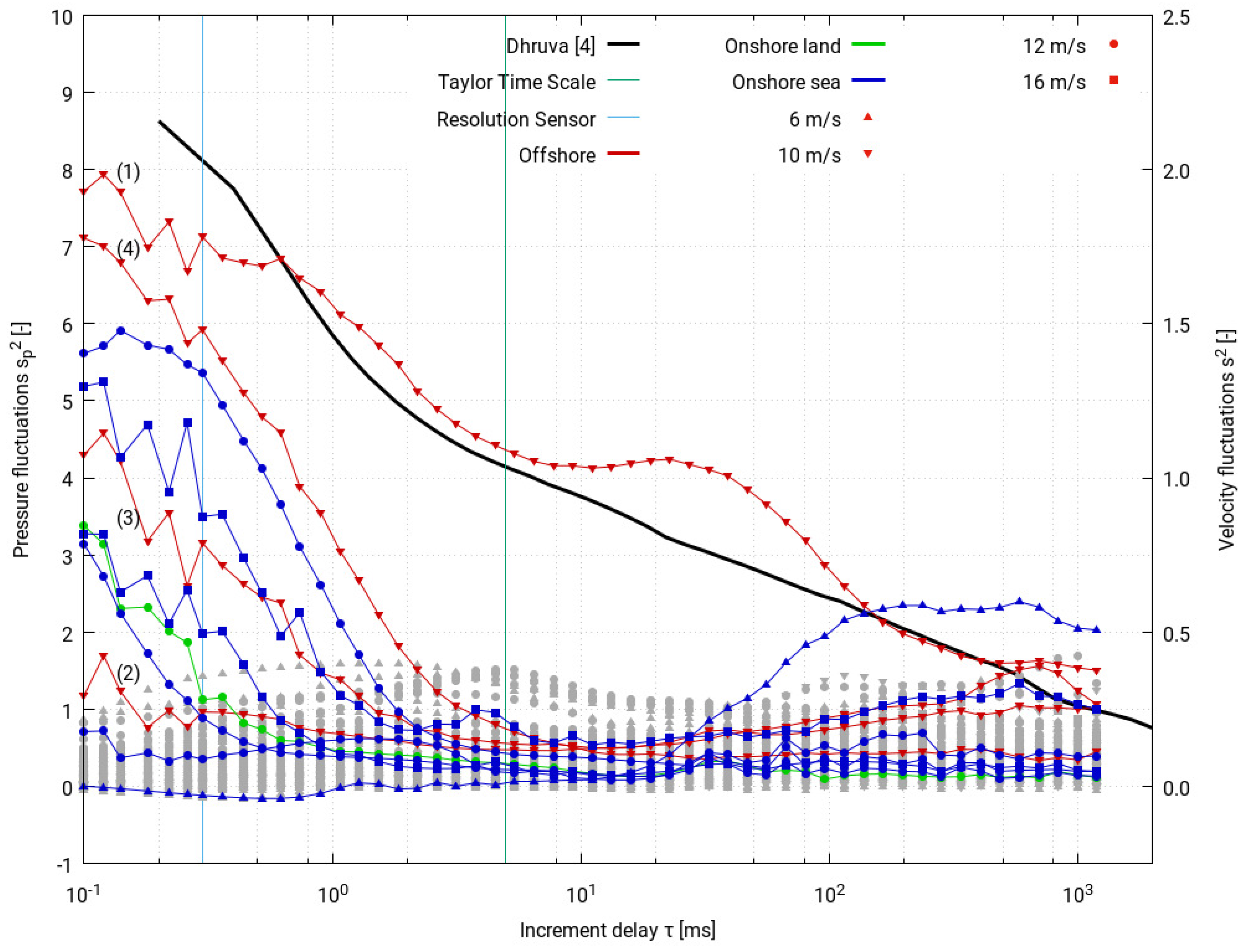
The computation of the shape parameter was straightforward, and the results are shown in Figure 4. The scale for the shape factor is shown on the left. Colors indicate locations, and symbols represent velocity classes. Time series with were grayed out, and will not be considered further in the following analysis. For purposes of comparison, shape factors from a particular velocity measurement ([25], = 7.6 m/s, = 1.36 m/s) were included (black line) as well.
The general behavior of both shape parameter functions for velocity and pressure was similar, whereas absolute values differed significantly. This behavior was also observed in reference [26]. Surprisingly, most of the pressure measurements resulted in close to zero.
We noted differences between the measurements of velocity and pressure concerning sampling rates and length of the time series.
In Figure 4, offshore curves are distinguished with numbers in brackets. They were all recorded on the same day with a short delay at the following times:
- (1)
- 19 October 2010, 8:44 a.m.
- (2)
- 19 October 2010, 8:54 a.m.
- (3)
- 19 October 2010, 8:55 a.m.
- (4)
- 19 October 2010, 8:57 a.m.
Pressure time series were recorded for a period of 100 s. For the first data set (1) was high. However, then, the pressure data resulted in until the values increased eight minutes later at (2). The time series (2), (3), and (4) were consecutive, so it can be said that the shape parameter for the turbulent pressure fluctuations did not remain constant in time for this interval. When all time series from 8:44 a.m. to 8:57 a.m.were concentrated into one and evaluated according to a common , a curve similar to the curve for velocity fluctuations was obtained. This has already been presented in reference [14].
We now try to relate these different statistical behaviors to the atmospheric boundary layer state. With our estimation of the Richardson number, a stability state was determined. Selected data from all our 119 measured data sets are shown in Table 1 and Table 2. Measurements with are marked with a star in the last column.
As can be seen from Table 1, high () behavior corresponded to unstable to neutral Atmospheric Boundary Layer (ABL) conditions: . However, a significant correlation with the Richardson number was not found.
4.1. Time Development of a Sample Time Series
Therefore, especially for the measurement on 19 October 2010, a possible transient behavior of the shape factor was investigated in more detail. The time development of measured data is presented in Table 2.
The measurements started at 8:44 a.m. when was high and the turbulence intensity from cup anemometers was low. In the following 7 min, the time series were found to have , with the mean velocity and potential temperature of the air remaining constant. Only the turbulence intensity increased from about 4 to about 8%.
At 8:54 a.m., the shape factor began to rise (see also curve (2) of Figure 4). Promptly, the turbulence intensity dropped more than 5.5 percentage points, and also, the potential temperature of the air decreased by 0.4 K with the rising shape factor.
Our interpretation is summarized as follows: the boundary layer, corresponding to time interval from 8:45 a.m. to 8:49 a.m. was stratified, and turbulent pressure fluctuations were distributed in a Gaussian way. At 8:50 a.m., a cluster of warm air rose up from the warmer sea surface to higher (and colder) regions ( consant, fluctuating). This may have led to a stronger vertical shear, thereby disturbing the (Gaussian) turbulent structures.
4.2. Occurrence Probabilities
As was seen in our evaluations of boundary layer states and shape factors, the occurrence of high values for (a highly non-Gaussian behavior) stems from a non-linear, dynamic process with chaotic phases, for which the term intermittency was introduced [27]. The occurrence probabilities for all of our 119 measurements are listed in Table 3.
In the first row, the number of states is listed for all measurements. We see much more unstable (84) than neutral (23) or stable (12) conditions. The subsequent two rows list the numbers for offshore and onshore locations with their states. In the fourth row, the tallies for high shape factor events are listed for all measurements. The probability for the occurrence of a high- event at a specific boundary layer state is shown in the next line. The same was done for both locations, offshore and onshore.
To correctly interpret the data, one has to know the circumstances of the measurements. The onshore measurements took place in spring 2008 between March and May. During this time of year, the ground begins to warm up slowly while the air heats up much faster, yielding stable conditions. Project specific constraints limited the offshore measurement campaign to a period in late summer and autumn 2010. At this time of year, the sea is still heated up from the summer and warms the air near the surface, while the air temperature subsides, and many unstable conditions can be observed.
The focus was laid on the onshore measurements for the relation between the boundary layer state and the occurrence of high shape factors in the turbulent pressure fluctuations. With a joint probability of about 16.7%, a high- was found for unstable and neutral states (7 out of 42, see Table 3). However, in stable conditions, a high- was not observed. So, we propose that turbulent fluctuations in the pressure may deviate from a normal distribution much more frequently under unstable or neutral boundary conditions than under stable conditions.
4.3. Confidence Considerations
To check the confidence of our above assumption, possible sources for errors were investigated. Individual measurements at onshore locations were recorded at different hours and days, so they can be assumed to be independently and randomly sampled. The probability of occurrence of a high event under combined unstable or neutral conditions was estimated to be . The statistical test was based on a binomial distribution with the states event occurred and no event occurred.
To check the occurrence probability of an event in the onshore stable boundary layer states, for the null-hypothesis, an occurrence probability was assumed to be the same as for unstable/neutral states, and finding no event was just bad luck. The alternative hypothesis postulates a much lower probability of for high- events under stable conditions (see Table 4).
The number of expected events for in onshore stable conditions is given in Table 4, and and were accepted if at least one event was found. However, no event of a non-Gaussian distribution was found under onshore stable conditions, and was rejected. The type I error rate was about 11.2%. This is also the level of significance (). To improve the statistical significance, the number of samples in stable conditions had to be raised up to 17 for (or 26 for ), but has not been done so far.
Since the offshore measurements were often consecutive within the same conditions, and no observations in neutral or stable conditions were acquired, the statistical confidence could not be estimated for the offshore turbulence. However, the calculated occurrence probability gave a good approximation to allow the quality of the type II error for the onshore unstable and neutral boundary layers to be checked. The setup for this test is presented in Table 5 and the errors were 11.4% for type I ( was rejected despite it being true) and 14.9% for type II ( was accepted when it was really false).
These error estimates were acceptable with the small number of measurements and the occurrence probability onshore was reasonable.
5. Impact on Boundary Layer Transition on a Wind Turbine Blade
In the preceding sections, we have described that small-scale turbulence below a Taylor’s length-scale of less than 50 mm are likely to show non-Gaussian behavior. We now briefly describe how this may be related to turbulent-laminar transitions on wind turbine blades. It has to be noted that more detailed investigations have been performed in the upper atmosphere for small aircraft [8,9]. Corresponding outdoor experiments on wind turbines were reported in reference [10,28]. It can be concluded that despite a high integral turbulence intensity of more that 10%, the energy content suitable for the receptivity of TS-waves is even smaller than in a wind-tunnel environment. More evidence for this low-frequency cut-off for aerodynamic important turbulence can be given by a simple argument to estimate an upper frequency for a boundary layer (BL) responding to an oscillating outer flow. Stokes [29], pp 191 ff, showed that this outer flow (with ) is damped out by viscosity according to with , being the kinematic viscosity and U being the main flow in the x-direction, with y being perpendicular to that. Now, if we introduce a Stokes boundary layer thickness by , we get . Here, we have set to an approximate value of 1 mm, a typical value for laminar boundary layers on airfoils at Reynolds numbers of several million. Therefore, this high-frequency, non-Gaussian regime may play an important role in triggering the TS-type of (blade) boundary layer instability on the pathway towards fully developed turbulence.
6. Conclusions
High-frequency (above 100 Hz) resolved measurements of pressure fluctuations for different average wind velocities under onshore and offshore conditions were investigated with respect to higher order statistical properties and were related to atmospheric boundary layer stability. It was found that up to a frequency of 4 kHz, pressure and velocity fluctuations obey the same power spectrum, and further, out of 119 time series in total, high shape factors were shown to occur with a total probability of about 10%, independent of the Taylor-length based Reynolds number. Sixty-four percent of all high shape factor events were recorded during unstable thermal stratification, and the level of occurrence seemed to be almost doubled when compared to onshore cases. When a continuous sequence of time series was investigated, strong variations of the shape factor were sometimes observed even during short periods of about half an hour.
We argue for a separation of time scales to distinguish between instationary and turbulent flow at about 100 Hz, because it is clear that a severe reduction of total turbulence intensity takes place which makes the usage of laminar airfoils (NACA 63-215, for example) meaningful.
Author Contributions
A.P.S. and A.J. conceived and designed the experiments; A.J. performed the experiments; A.P.S. and A.J. analyzed the data; A.P.S. wrote the paper.
Funding
We thank the State of Schleswig-Holstein, Ministry of Science, Economics and Transportation for funding this project under Contract No.122-09-023.
Acknowledgments
We would like to thank the Germanischer Lloyd/Garrad Hassan (formerly WINDTEST) for their support during the measurement periods, onshore as well as offshore. We thank the Department of Physics at the University of Oldenbourg for their beneficial assessments and testing of our pressure sensors. Our thanks go also to the Deutscher Wetterdienst (DWD) for providing additional local temperature data. Discussion with S. Emeis, Institute of Meteorology and Climate Research, Karlsruhe Institute of Technology, Germany, is gratefully acknowledged.
Conflicts of Interest
The authors declare no conflict of interest.
References
- Schaffarczyk, A. (Ed.) Understanding Wind Power Technology; Wiley: Chichester, UK, 2014. [Google Scholar]
- Schaffarczyk, A.P. Introduction to Wind Turbine Aerodynamics; Springer: Berlin, Germany, 2014. [Google Scholar]
- Emeis, S. Wind Energy Meteorology; Springer: Heidelberg, Germany, 2013. [Google Scholar]
- Obukhov, A.M. Turbulence in an atmosphere with a non-uniform temperature. Bound.-Lay. Metereol. 1971, 2, 7–29. [Google Scholar] [CrossRef]
- Kaimal, J.; Finnigan, J. Atmospheric Boundary Layer Flows: Their Structure and Measurements; Oxford University Press: Oxford, UK, 1994. [Google Scholar]
- Mahrt, L.; Vickers, D.; Howell, J.; Høstrup, J.; Wilzak, J.; Edson, J.; Hare, J. Sea surfuace drag coeficiecient in the Risøe Air Sea Experiment. J. Geophys. Res. 1996, 14, 327–335. [Google Scholar]
- Grachev, A.; Leo, L.; Fernando, H.; Fairall, C.; Creegan, E.; Blomquist, B.W.; Christman, A.; Hocut, C. Air-sea/land interaction in the costal zone. Bound.-Lay. Meteorol. 2018, 167, 181–210. [Google Scholar]
- Reeh, A.D.; Weissmüller, M.; Tropea, C. Free-Flight Investigation of Transition under Turbulent Conditions on a Laminar Wing Glove. In Proceedings of the 51st AIAA Aerospace Sciences Meeting, Grapevine, TX, USA, 7–10 January 2013. [Google Scholar]
- Reeh, A.D.; Tropea, C. Behaviour of a natural laminar flow airfoil in flight through atmospheric turbulence. J. Fluid Mech. 2015, 767, 394–429. [Google Scholar] [CrossRef]
- Schaffarczyk, A.; Schwab, D.; Breuer, M. Experimental detection of Laminar-Turbulent Transition on a rotating wind turbine blade in the free atmosphere. Wind Energy 2016, 19. [Google Scholar] [CrossRef]
- Schwab, D. Aerodynamische Grenzschichtuntersuchungen an Einem Windturbinenblatt im Freifeld. Ph.D. Thesis, Helmut-Schmidt-Universität, Hamburg, Germany, 2018. [Google Scholar]
- Beck, C. Superstatistics in hydrodynamic turbulence. Physica D 2004, 193, 195–207. [Google Scholar] [CrossRef] [Green Version]
- Castaing, B.; Gagne, Y.; Hopfinger, E. Velocity probability density functions of high Reynolds number turbulence. Physica D 1990, 64, 177–200. [Google Scholar] [CrossRef]
- Jeromin, A.; Schaffarczyk, A.P. Advanced statistical analysis of high-frequency turbulent pressure fluctuations for on- and off-shore wind. In Proceedings of the EUROMECH Colloquium 528: Wind Energy and the Impact of Turbulence on the Conversion Process, Oldenburg, Germany, 22–24 February 2012. [Google Scholar]
- Jeromin, A.; Schaffarczyk, A.P. Relating high-frequency offshore turbulence statistics to boundary layer stability. In Proceedings of the 2013 International Conference on Aerodynamics of Offshore Wind Energy Systems and Wakes (ICOWES2013), Frankfurt, Germany, 19–21 November 2013; Shen, W.Z., Ed.; 2013; pp. 162–172. [Google Scholar]
- Segalini, A.; Ramis, O.; Schlatter, P.; Henrik Alfredsson, P.; Rüedi, J.D.; Alessandro, T. A method to estimate turbulenFphysicace intensity and transvers Taylor microscale in turbulent flows from spatially averaged hot-wire data. Exp. Fluids 2011, 51, 693–700. [Google Scholar] [CrossRef]
- Jeromin, A.; Schaffarczyk, A.P. Statistische Auswertungen Turbulenter Druckfluktuationen auf der Off-Shore Messplattform FINO3; Technical Report Unpublished Interal Report No. 78; University of Applied Sciences Kiel: Kiel, Germany, 2012. [Google Scholar]
- Lück, S.; Renner, C.; Peinke, J.; Friedrich, R. The Markov-Einstein coherence length—An new meaning for the Taylor length in turbulence. Phys. Lett. 2006, 359, 335–338. [Google Scholar] [CrossRef]
- Batchelor, G. Pressure fluctuations in isotropic turbulence. Proc. Camb. Philos. Soc. 1951, 47, 359–374. [Google Scholar] [CrossRef]
- Xu, H.; Ouellette, T.; Vincenzi, D.; Bodenschatz, B. Acceleration correlations and pressure structure functions in high-reynolds number turbulence. Phys. Rev. Lett. 2007, 99, 204501. [Google Scholar] [CrossRef] [PubMed]
- Sathe, M.; Mann, J.; Barlas, T.; Bierbooms, W.; van Bussel, G. Influence of atmospheric stability on wind turbine loads. Wind Energy 2013, 16, 1013–1032. [Google Scholar] [CrossRef]
- Coelingh, J.; van Wijk, A.; Holtslag, A. Analysis of wind speed observations over the North Sea. J. Wind Eng. Ind. Aerodyn. 1996, 61, 51–69. [Google Scholar] [CrossRef]
- Oost, W.; Jacobs, C.; van Oort, C. Stability effects on heat and moisture fluexes at sea. Bound.-Lay. Meteorol. 2000, 95, 271–302. [Google Scholar] [CrossRef]
- Emeis, S. Upper limit for wind shear instable stratified conditions expressed in terms of a bulk Richardson number. Meteorol. Z. 2017, 16, 421–430. [Google Scholar] [CrossRef]
- Dhruva, B. An Experimental Study of High Reynolds Number Turbulence in the Atmosphere. Ph.D. Thesis, Yale University, New Haven, CT, USA, 2000. [Google Scholar]
- Jeromin, A.; Schaffarczyk, A.; Puczylowski, J.; Peinke, J.; Hoelling, M. Highy resolved measurements of atmospheric turbulence with the new 2D-atmospheric Laser Cantilever Anemometer. J. Phys. Conf. Ser. 2014, 555. [Google Scholar] [CrossRef]
- Lohse, D.; Grossmann, S. Intermittency in turbulence. Physica A 1993, 194, 519–531. [Google Scholar] [CrossRef]
- Madsen, H.; Fuglsang, P.; Romblad, J.; Enevoldsen, P.; Laursen, J.; Jensen, L.; Bak, C.; Paulsen, U.S.; Gaunna, M.; Sorensen, N.N.; et al. The DAN-AERO MW experiments. AIAA 2010, 645. [Google Scholar] [CrossRef]
- Batchelor, G. An Introduction to Fluid Dynamics; Cambridge University Press: Cambridge, UK, 1967. [Google Scholar]
Figure 1.
Pressure sensor after six months of offshore service (diameter = 12 mm).

Figure 2.
Locations of onshore (Kaiser–Wilhelm–Koog) and offshore (FINO3 platform) test sites, 80 km west of the island of Sylt. ©FEZ FH Kiel GmbH, Graphics: Bastian Barton.
Figure 2.
Locations of onshore (Kaiser–Wilhelm–Koog) and offshore (FINO3 platform) test sites, 80 km west of the island of Sylt. ©FEZ FH Kiel GmbH, Graphics: Bastian Barton.

Figure 3.
Installation of two parallel pressure sensors (T1 and T2) at the FINO3 platform.

Figure 4.
Shape parameters for all collected measurements. Colors represent locations: offshore, onshore with wind coming from land or sea side. The symbols represent the velocity classes for the wind speed. Measurements with are shown in grey. For reasons of comparison, Taylor’s and Kolmogorov’s time scales are given in 5 msec and 0.05 msec, respectively. The sensor’s resolution goes down to approximately 0.3 msec only.


Table 1.
Summary of selected Atmospheric Boundary Layer (ABL) stability cases: wind speeds () and turbulence intensities () from cup anemometers, numbers and estimated ABL states.
Table 1.
Summary of selected Atmospheric Boundary Layer (ABL) stability cases: wind speeds () and turbulence intensities () from cup anemometers, numbers and estimated ABL states.
| Date & Time | Location | (m/s) | Ti (%) | Ri (-) | Boundary Layer State | |
|---|---|---|---|---|---|---|
| 21 October 2010, 7:56 a.m. | Offshore | 06.6 | 08.2 | −0.54 | Unstable | |
| 28 April 2008, 9:35 a.m. | Onshore | 06.1 | 11.9 | −0.15 | Unstable | |
| 19 October 2010, 8:57 a.m. | Offshore | 10.8 | 02.2 | −0.13 | Unstable | * |
| 19 October 2010, 8:44 a.m. | Offshore | 10.2 | 03.1 | −0.12 | Unstable | * |
| 19 August 2010, 8:13 a.m. | Offshore | 12.7 | 02.8 | −0.06 | Unstable | |
| 25 March 2008, 2:55 p.m. | Onshore | 11.3 | 10.8 | −0.03 | Unstable | * |
| 29 March 2008, 11:44 a.m. | Onshore | 15.3 | 10.6 | −0.01 | Neutral | |
| 30 March 2008, 6:04 p.m. | Onshore | 15.7 | 05.6 | 00.00 | Neutral | * |
| 28 April 2008, 2:20 p.m. | Onshore | 05.8 | 02.1 | 00.01 | Neutral | * |
| 1 May 2008, 2:55 a.m. | Onshore | 06.0 | 06.0 | 00.10 | Stable | |
| 12 April 2008, 7:24 p.m. | Onshore | 05.2 | 11.0 | 00.28 | Stable |
Table 2.
Development of Time Series on October 19. Potential temperatures (), wind speeds () and turbulence intensities () from cup anemometers, numbers, and estimated ABL states.
Table 2.
Development of Time Series on October 19. Potential temperatures (), wind speeds () and turbulence intensities () from cup anemometers, numbers, and estimated ABL states.
| Time | (K) | (K) | (m/s) | Ti (%) | Ri (-) | Boundary Layer State | |
|---|---|---|---|---|---|---|---|
| 8:44 a.m. | 283.6 | 286.8 | 10.2 | 03.1 | −0.12 | Unstable | * |
| 8:45 a.m. | 283.5 | 286.8 | 10.2 | 03.9 | −0.13 | Unstable | |
| 8:47 a.m. | 283.4 | 286.8 | 10.0 | 07.5 | −0.14 | Unstable | |
| 8:49 a.m. | 283.4 | 286.8 | 10.1 | 07.3 | −0.13 | Unstable | |
| 8:50 a.m. | 283.5 | 286.8 | 09.3 | 06.7 | −0.16 | Unstable | |
| 8:52 a.m. | 283.5 | 286.8 | 11.2 | 06.0 | −0.11 | Unstable | |
| 8:54 a.m. | 283.5 | 286.8 | 10.8 | 07.7 | −0.11 | Unstable | * |
| 8:55 a.m. | 283.2 | 286.8 | 11.2 | 04.2 | −0.12 | Unstable | * |
| 8:57 a.m. | 283.1 | 286.8 | 10.8 | 02.2 | −0.13 | Unstable | * |
Table 3.
Correlation of the occurrence probability of a high shape factor to boundary layer state for all 119 measurements.
Table 3.
Correlation of the occurrence probability of a high shape factor to boundary layer state for all 119 measurements.
| Boundary Layer State | ||||
|---|---|---|---|---|
| Unstable | Neutral | Stable | Total | |
| All | 84.0 | 23.0 | 12.0 | 119.0 |
| Offshore | 65.0 | 00.0 | 00.0 | 065.0 |
| Onshore | 19.0 | 23.0 | 12.0 | 054.0 |
| All | 07.0 | 04.0 | 00.0 | 011.0 |
| Probability (%) | 08.3 | 17.4 | 00.0 | 009.2 |
| Offshore | 04.0 | 00.0 | 00.0 | 004.0 |
| Probability (%) | 06.2 | -/- | -/- | 0-/- |
| Onshore | 03.0 | 04.0 | 00.0 | 007.0 |
| Probability (%) | 15.8 | 17.4 | 00.0 | 0-/- |
Table 4.
Error estimation for the occurrence of non-Gaussian turbulence for onshore stable conditions.
Table 4.
Error estimation for the occurrence of non-Gaussian turbulence for onshore stable conditions.
| Hypotheses: | |
|---|---|
| Occurrence probability is in stable conditions | |
| Occurrence probability is in stable conditions | |
| Error Type I | |
| Number of samples | 12 |
| Occurrence probability | |
| Expected occurrences | |
| Variance | |
| Acceptance region for | {1…12} |
| Rejection region for | {0} |
| Probability of error | 11.2% |
Table 5.
Error estimation for the occurrence of non-Gaussian turbulence for the onshore unstable/neutral conditions.
Table 5.
Error estimation for the occurrence of non-Gaussian turbulence for the onshore unstable/neutral conditions.
| Hypotheses: | ||
|---|---|---|
| Occurrence probability is in unstable/neutral conditions | ||
| Occurrence probability is in unstable/neutral conditions | ||
| Error Type I | Error Type II | |
| Number of samples | 42 | |
| Occurrence probability | ||
| Expected occurrences | ||
| Variance | ||
| Acceptance region for | {0…4} | |
| Rejection region for | {5…42} | |
| Probability of error | 11.4% | 14.9% |
© 2018 by the authors. Licensee MDPI, Basel, Switzerland. This article is an open access article distributed under the terms and conditions of the Creative Commons Attribution (CC BY) license (http://creativecommons.org/licenses/by/4.0/).
Share and Cite
MDPI and ACS Style
Schaffarczyk, A.P.; Jeromin, A. Measurements of High-Frequency Atmospheric Turbulence and Its Impact on the Boundary Layer of Wind Turbine Blades. Appl. Sci. 2018, 8, 1417. https://doi.org/10.3390/app8091417
AMA Style
Schaffarczyk AP, Jeromin A. Measurements of High-Frequency Atmospheric Turbulence and Its Impact on the Boundary Layer of Wind Turbine Blades. Applied Sciences. 2018; 8(9):1417. https://doi.org/10.3390/app8091417
Chicago/Turabian StyleSchaffarczyk, Alois Peter, and Andreas Jeromin. 2018. "Measurements of High-Frequency Atmospheric Turbulence and Its Impact on the Boundary Layer of Wind Turbine Blades" Applied Sciences 8, no. 9: 1417. https://doi.org/10.3390/app8091417
Note that from the first issue of 2016, this journal uses article numbers instead of page numbers. See further details here.