An Improved Analytical Algorithm on Main Cable System of Suspension Bridge

Featured Application

An improved analytical algorithm has been successfully applied in shape finding during design and configuration control during construction of main cable system for suspension bridges.

Abstract

This paper develops an improved analytical algorithm on the main cable system of suspension bridge. A catenary cable element is presented for the nonlinear analysis on main cable system that is subjected to static loadings. The tangent stiffness matrix and internal force vector of the element are derived explicitly based on the exact analytical expressions of elastic catenary. Self-weight of the cables can be directly considered without any approximations. The effect of pre-tension of cable is also included in the element formulation. A search algorithm with the penalty factor is introduced to identify the initial components for convergence with high precision and fast speed. Numerical examples are presented and discussed to illustrate the accuracy and efficiency of the proposed analytical algorithm.

1. Introduction

Cable-supported structures, such as suspension bridges, have been recognized as the most appealing structures due to their aesthetic appearance as well as the structural advantages of cables [1,2,3,4]. It is well known that cables cannot behave as structural members until large tensioning forces are induced, such as pre-stressed cable in structures [5]. Therefore, in order to design a cable-supported structure economically and efficiently, it is extremely important to determine the optimized initial cable tensions or unstrained lengths.

Generally, designers cannot determine the initial shape arbitrarily when the cable structures are considered. The initial shape is determined while satisfying the equilibrium condition between dead loads and internal member forces, including cable tensions in the preliminary design stage because cable members display strongly geometric nonlinear behavior as well as the configuration of a cable system cannot be defined in stress-free state. The process determining the initial state of cable structures is referred to as ‘‘shape finding ’’, ‘‘form finding ’’, or‘‘ Initial shape or initial configuration’’ [6,7,8,9,10,11].

Until now, nonlinear analysis procedures have been developed for shape finding problems of cable bridges: the trial-and-error method [12], the initial force method [10,13], the analytical and iteration method [14,15], the target configuration under dead loads (TCUD) related methods [9], the optimization method [16,17], and the combined method [18].

Above mentioned various form-finding approaches are generally into three categories: (1) the simplified approach; (2) the Finite Element (FE)-based approach; and (3) the analytical method.

The simplified method assumes that the load acts uniformly along the span of the main cable, which follows a parabolic shape [2,17,19]. To account for a cable’s sag effect, Ernst proposed the equivalent modulus of elasticity for a parabolic cable [20]. The simplicity of Ernst’s formula has made it widely used not only in the research field, but also for the practical designs of suspension bridges. Owing to its simplicity, this approach has been adopted by several investigators [21,22,23], and has been proved to be sufficient for some cases. Namely, when a cable has relatively high stress and small length, the Ernst equivalent modulus approach could achieve a good result. However, the parabolic approximation becomes inaccurate for cables with a large sag-to-span ratio (>1/8), which experience self-weight along the length of the cable and concentrated forces from the hangers.

To improve the accuracy and facilitate nonlinear analyses of suspension bridges, various FE-based approaches have been developed. In these approaches, most of the finite element packages are still lack of suitable cable elements. A sagging cable is often simulated as two-node element, multi-node element, and curved element with rotational degrees of freedom [24,25,26]. The two-node element is only suitable for modeling the cables with high pretension and small length [27,28], and equivalent modulus are used to account for the sag effect. For cables with large sag, a series of straight elements is used to model the curved geometry of cables. The multi-node element is based on the higher order polynomials for the interpolation functions [29,30]. The tangent stiffness matrix and nodal force vector are obtained while using the iso-parametric formulation. These elements give accurate results for cables with small sag. For cable element with large sag, it is necessary to use a large number of elements to model the curved geometry of cable. Therefore, it causes computational costs.

These FE-based approaches identify the target configuration of main cable via updating nodal positions and internal tension of cable elements based on nonlinear structural analysis. However, these FE-based approaches elevate the computational effort, and their convergence depends to a large extent on the assumed initial cable configuration and forces.

The alternative approach is based on exact analytical expressions for the elastic catenary, since the equilibrium configuration of a hanging cable is a catenary in nature. This method was originally proposed by O’Brien and Francis [31] and was later extensively developed [32,33,34,35,36]. In particular, there are various catenary-type analytical elements available, which can be used to model large sag cables in suspension bridges:

(1) Inextensible catenary elements: The cable elements adopted are infinitely stiff in the axial direction and cannot experience any increment of length. In practice, computer applications that are based on this type of element encounter severe difficulties, solving procedures tend to experience large numerical instability, causing a very difficult or even impossible convergence.

(2) Elastic catenary elements: An elastic catenary curve is defined as the curve formed by a perfectly elastic cable, which obeys Hooke’s law and has negligible resistance to bending, when being suspended from its ends and subjected to gravity. It should be noted that the conventional formulations are based on the hypothesis of small deformations, meaning that the forces are integrated with respect to the initial configuration of the catenary. Hence, the weight per unit length does not vary consistently with the elongation of the catenary. This may result in an inaccurate equilibrium of forces in the deformed configuration.

The main advantages of the catenary-type cable elements are the reduction of degrees of freedom, the simplicity of finding the dead load geometry of the cable system, the exact treatment of cable sag, the exact treatment of cable weight as it is included in the equations used for element formulation, and the simplicity of including the effect of pre-tension of the cable by simply giving the unstressed cable length. However, the cable segment equation is unsolvable when the initial three components are not set properly because of the so-called initial value sensitivity.

The purpose of this paper is to develop a catenary cable element for the nonlinear analysis of cable structures that are subjected to static loadings. Firstly, the tangent stiffness matrix and internal force vector of the element are derived explicitly based on the exact analytical expressions of elastic catenary. Self-weight of the cables can be directly considered without any approximations. The effect of pre-tension of cable is also included in the element formulation. Then, a search algorithm with the penalty factor is introduced to satisfy the convergence requirement with high precision and fast speed. Finally, numerical examples are presented and discussed to illustrate the accuracy and efficiency of the proposed analytical algorithm.

2. Segmental Catenary Theory of Main Cable

To accurately simulate the realistic behavior of main cables, the catenary element exactly considering the effects of cable sags, cable self-weight, and cable pretension is used.

2.1. Basic Equations

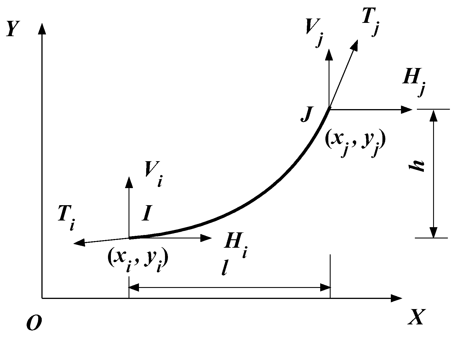
An elastic catenary cable element has been derived from the exact solution of the elastic catenary cable equation, deformed due to its self-weight [32,33]. It can be formulated in three dimensional coordinates, but only two-dimensional formulation is described in this study.

Consider a cable segment suspended between points i(x_i, y_i) and j(x_j, y_j), as shown in Figure 1. It is assumed that the cable:

(1)

is perfectly flexible and can sustain only tensile forces;

(2)

is composed of a homogeneous material which is linearly elastic;

(3)

is subjected to a uniform distributed load q along the cable length; and,

(4)

the tensile stiffness of the cable is calculated using the cross-section before deformation.

The relative distances between two nodes (i, j) along the global x, y axis, are denoted as l (l = x_j − x_i) and h (h = y_j − y_i), respectively, in Figure 1, which can be expressed as a function of the global nodal force H_i and V_i at the node i as:

$$l=-\frac{H_i·S_0}{EA}-\frac{H_i}{q}\left\{\ln \left(V_i+\sqrt{H_i^2+V_i^2}\right)-\ln \left(V_i-S_0·q+\sqrt{H_i^2+{(V_i-S_0·q)}^2}\right)\right\}$$

(1)

$$h=\frac{q·S_0^2-2V_i·S_0}{2EA}-\frac{1}{q}\left[\sqrt{H_i^2+V_i^2}-\sqrt{H_i^2+{(V_i-S_0·q)}^2}\right]$$

(2)

The force equilibriums of the elastic catenary cable require that:

$$\{\begin{array}{l}-H_i=H_j=H\\ V_j=-V_i+S_{0}q\\ T_i=\sqrt{H_i^2+V_i^2}\\ T_j=\sqrt{H_j^2+V_j^2}\end{array}$$

(3)

Equations (1) and (2) are defined as the basic equations for segmental catenary cable, showing the relation between the segmental forces and geometric parameters. Generally, the main cable is divided into several segments (number N), each segment establishes two basic equations, in total 2 times of N equations are obtained for the whole main cable system. In Equations (1)–(3), E is the elastic modulus; A is the cross sectional area, q is the self-weight of the unstressed main cable; l represents the span length of the cable segment, h represents the elevation difference of two ends, and S₀ represents the unstressed length of cable segment; T_i, T_j are the cable tension at the left (i) and right (j) ends of the cable segment, respectively; H_i and H_j are the horizontal component of cable tension at the left (i) and right (j) ends of the cable segment, respectively; and, V_i and V_j are the vertical component of cable tension of the left(i) and right (j) ends of the cable segment, respectively.

From Equations (1) and (2), it can be found that for a cable segment with determined S₀, H, and V_i, the length l, and high difference h can be easily obtained; similarly, for a cable segment with determined S₀, l, and h, the internal forces H and V can be easily solved. Thus, only three independent variables exist in these five variables (S₀, H, V_i, l and h).

2.2. Stiffness Formulation

Following describe the procedure of stiffness formulation of the elastic catenary cable element. Considering q, S₀, EA as constants, partial differentiation of both sides of Equations (1) and (2) yield the following incremental relationships between the relative nodal displacements and nodal forces.

$$\left\{\begin{array}{l}dH\\ dV\end{array}\right\}=\left[K\right]\left\{\begin{array}{l}dx\\ dy\end{array}\right\}$$

(4)

$$\left[K\right]=\left[\begin{array}{l}{K}_{11}{K}_{12}\\ K_{11}{K}_{22}\end{array}\right]={\left[B\right]}^{-1}$$

(5)

$$\left[B\right]=\left[{\displaystyle \sum _{m=1}^{i}b}\right]=\left[\begin{array}{l}{\displaystyle \sum _{m=1}^i{b}_{11}}{\displaystyle \sum _{m=1}^i{b}_{12}}\\ {\displaystyle \sum _{m=1}^i{b}_{21}}{\displaystyle \sum _{m=1}^i{b}_{22}}\end{array}\right]$$

(6)

$$\{\begin{array}{l}dH=d{H}_i^{(k)}=d{H}_i^{(k-1)}=d{H}_L\\ dV=d{V}_i^{(k)}=d{V}_i^{(k-1)}=d{V}_L\end{array}$$

(7)

$$b_{11}=\frac{\partial l}{\partial H_i}=-\left(\frac{S_0}{EA}+\frac{1}{q}\ln \frac{T_j+V_j}{T_i-V_i}\right)-\frac{H_i^2}{q}\left[\frac{1}{T_j\left(T_j+V_j\right)}-\frac{1}{T_i\left(T_i-V_i\right)}\right]$$

(8)

$$b_{12}=b_{21}=-\frac{H_i}{q}\left[\frac{1}{T_j}-\frac{1}{T_i}\right]$$

(9)

$$b_{22}=-\frac{S_0}{EA}-\frac{1}{q}\left[\frac{V_j}{T_j}+\frac{V_i}{T_i}\right]$$

(10)

where: [K] is the stiffness matrix due to cable shape change from end point (e.g., left end) to segment point i; if the segment point i become the other end point (e.g., right end), [K] is the stiffness matrix of the main cable for the whole span; dx, dy are the cumulative amount of change in span and elevation respectively from end point to segment point i; and, dH_i^(k), dV_i^(k) are the increment horizontal and vertical component of cable force at segment i, respectively.

2.3. General Solution Procedure

The tangent stiffness matrix and internal force vector of cable element are determined while using an iterative procedure. This procedure requires the initial values of end forces (H, V). The iterative procedure for obtaining tangent stiffness matrix and internal force vector of cable element is briefly presented, as follows:

(1)

input q, E, A, S₀, nodes I (x_i, y_i) and J (x_j, y_j);

(2)

calculate l₀ = x_j − x_i, h₀ = y_j − y_i;

(3)

initialize end forces (H, V);

(4)

update (l, h) using Equations (1) and (2);

(5)

calculate incompatibility vector of relative distances ds = {dl dh}^T;

(6)

if ds is smaller than the permissible tolerances, calculate [K] using Equation (5) and internal forces using Equation (3), otherwise continue to next step;

(7)

calculate the correction vector of end forces {dH, dV}using Equation (4);

(8)

update the end forces H_i+1 = H_i + dH, V_i+1 = V_i + dV and go to Step (4).

2.4. No Solution Cases for Cable Segment Equation

The solution to the governing equation requires the Newton-Raphson type iteration while using initial trials of the force vector of the left node in the first cable element. However, the convergence of the gradient-based Newton-Raphson approach strongly depends on the initial value, and the estimation of initial value remains a challenge.

Generally, there are two states for numerical analysis of main cable system: one is the main cable system at finished state for the whole bridge; the other is at construction state, only the main cable installation is finished [37]. The tension force at one end need to be assumed (or determined) for the main cable system calculation, the coordinates are iterated with convergence conditions. At the finished state, the tension force at one end and the horizontal distance between two ends are given, the unstressed cable length and the elevation between two end points can be solved, that is, l, H_i, V_i are known, to solve S₀, h. If the end tension force is assumed unreasonably, then there will be no solution for Equations (1) and (2).

To solve unstressed length S₀, Equation (1) is rewritten as:

$$f\left(S_0\right)=-\frac{H_i·S_0}{EA}-\frac{H_i}{q}\left\{\ln (V_i+\sqrt{H_i^2+V_i^2})-\ln (V_i-S_0·q+\sqrt{H_i^2+{(V_i-S_0·q)}^2}\right\}-l$$

(11)

Suppose that l, H_i, EA are constants, and EA > 0, q > 0, 0 < S₀ < 5000 m (the length of main cable for single-span suspension bridge is currently less than 5000 m), there will be no solution for Equation (1) in the following three conditions:

Condition 1.

When V_i is positive and the absolute value of V_i is large enough, l and H_i have the same sign, there will be no solution for Equation (1). It can be proved, as follows:

$$f\left(S_0\right)=-\frac{H_i·S_0}{EA}-\frac{H_i}{q}\ln \frac{1+\sqrt{\frac{H_i^2}{V_i^2}+1}}{1-\frac{S_0·q}{V_i}+\sqrt{\frac{H_i^2}{V_i^2}+\frac{{(V_i-S_0·q)}^2}{V_i^2}}}-l\approx -\frac{H_i·S_0}{EA}-\frac{H_i}{q}\ln 1-l=-\frac{H_i·S_0}{EA}-l\ne 0$$

(12)

Condition 2.

When V_i is negative and the absolute value of V_i is large enough, l and H_i have the same sign, there will be no solution for Equation (1). It can be proved, as follows:

$$\begin{array}{l}f\left(S_0\right)=-\frac{H_i·S_0}{EA}-\frac{H_i}{q}\ln \frac{1-\sqrt{\frac{H_i^2}{V_i^2}+1}}{1-\frac{S_0·q}{V_i}-\frac{V_i-S_0·q}{V_i}\sqrt{1+\frac{H_i^2}{{(V_i-S_0·q)}^2}}}-l\\ \approx -\frac{H_i·S_0}{EA}-\frac{H_i}{q}\ln \frac{1-\left(1+\frac{1}{2}\frac{H_i^2}{V_i^2}\right)}{1-\frac{S_0·q}{V_i}-\left(1-\frac{S_0·q}{V_i}\right)\left[1+\frac{1}{2}\frac{H_i^2}{{(V_i-S_0·q)}^2}\right]}-l\approx -\frac{H_i·S_0}{EA}-l\ne 0\end{array}$$

(13)

Condition 3.

When the absolute value of V_i is small enough, l and H_i have the same sign, Equation (14) is obtained from Equation (11), there will be no solution for Equation (1), It can be proved, as follows:

$$f\left(S_0\right)=-H_i\left(\frac{S_0}{EA}+\frac{1}{q}\ln \frac{\left|H_i\right|}{\sqrt{H_i^2+{\left(S_0·q\right)}^2}-S_0·q}\right)-l<-H_i\frac{S_0}{EA}-l\ne 0$$

(14)

3. Improved Numerical Analysis Method

In order to solve the problem that no solution for basic equations since tension force at one end of the cable was assumed unreasonable, an improved numerical analysis method is proposed though searching the reasonable initial tension force at one end of the cable.

Main cable system calculation in the main span and side span can be divided into two cases: one is that the theoretical vertex position is known; the other is that the saddle position is known. In the first case, the tangent point position between saddle and main cable need not to be corrected, while in the second case, the tangent point position between saddle and main cable need to be corrected. The first case is the special case of the second case [37].

When theoretical vertex position and saddle position are known, the calculation of main cable system in main span can adopt two iterative methods: one is the specified point elevation (or un-stressed cable length) iterates step by step, the other is the specified point elevation (or un-stressed cable length) iterates once [31]. However, the calculation of main cable system in side span generally adopts the method that the un-stressed cable length is iterated once.

3.1. The Main Cable System Calculation in Main Span at Finished State

The stiffness due to cable shape change, as mentioned in Section 2.2, should be determined first, when the iterative method was used to calculate the designated point elevation (or un-stressed cable length) for main cable system in main span.

3.1.1. Determination of Cable Force Adjustment at Start Point

Equation (4) is obtained while ignoring the higher order terms of the Taylor series, which is an approximate expression. Due to strong nonlinear of suspension cable, the iterative methods for determining horizontal and vertical component of cable force adjustment at start point by Equation (4) sometimes fail to converge. Therefore, we need to revise the adjustment amount as the following Equation (15):

$$\{\begin{array}{l}{H}_L=H_{L0}+\alpha ·dH\\ V_L=V_{L0}+\alpha ·dV\end{array}$$

(15)

where, H_L0, V_L0 are the initial value of horizontal and vertical component of cable force at left start end, respectively; α is called penalty factor (or Newton-Downhill factor) in the range from 0 to 1.

Obviously, if the horizontal and vertical component of initial cable force adjustment amount are much less than the value before adjustment, which means that the non-linear property of the cable force adjustment process is not strong, then α = 1; otherwise, α should be chosen between 0.1 and 1. Thus, the iteration can converge with high efficiency. The value of α is determined based on the above principle, and calculated, as follows:

$$\{\begin{array}{l}\alpha =0.1\frac{\sqrt{H_{L0}^2+V_{L0}^2}}{\sqrt{{\left(dH\right)}^2+{\left(dV\right)}^2}};if\left|dH\right|>0.1\left|H_{L0}\right|or\left|dV\right|>0.1\left|V_{L0}\right|\\ \alpha =1;if\left|dH\right|\le 0.1\left|H_{L0}\right|and\left|dV\right|\le 0.1\left|V_{L0}\right|\end{array}$$

(16)

3.1.2. Improved Numerical Analysis Method and Its Iteration Steps

The main cable system calculation in main span under the condition that theoretical vertex position is known using step by step iteration method is illustrated as an example, and the iteration steps are shown in the following:

Step 1

All vertical loads in main span were simplified as uniform distributed load along the span, and the internal forces at both support ends H₁(1:2), V₁(1:2) were calculated using traditional parabola theory (actually only the internal force at start point is needed).

Step 2

The start end forces H₁(1:2), V₁(1:2) were regarded as the reference value H(1:2), V(1:2) of initial iterated internal forces.

Step 3

Input H(1:2), V(1:2) into iterative equations, and determine whether the iterative equations were solvable or not, and set initial value to sign IBZ, IBZ ⇐ 1 (Note: IBZ = 1, solvable; IBZ = 0, unsolvable).

Step 4

J2 ⇐ 1 (J2 is the modification times of iterated initial internal force when there is no solution for iterative equations)

Step 5

If IBZ = 0, obtain correction factor according to J2, modify the overall level of initial iterated internal forces (this algorithm called search algorithm, which searching a suitable internal force at start point by changing J2 to make the iterative equation solvable), namely:

$$J2\Leftarrow J2+1;$$

$$C3\Leftarrow 1+{\left(-1\right)}^{\left[J2-\mathrm{int}\left(\frac{J2}{2}\right)\times 2+1\right]}\times \mathrm{int}\left(\frac{J2+1}{2}\right)\times 0.05;$$

$$H(1:2)\Leftarrow C3\times H1(1:2);$$

$$V(1:2)\Leftarrow C3\times V1(1:2);$$

If IBZ = 1, go to Step 6.

Step 6

On the basis of Step 5 or Step 2, we determine the initial iteration horizontal force multiplier (KK) at start point, and get the elevation error at different points. Then, find suitable initial horizontal force iteration multiplier, and obtain the internal force and deformation in the main span by secant method, go to Step 7.

If there is no solution, then IBZ = 0, go to Step 5 (i.e., correcting overall level of initial iterated internal forces). The details of step 6 are shown in the following:

Step 6.1

Set initial iteration horizontal force, vertical force at start point:

H0(1) ⇐ KK × H(1),V 0(1) ⇐ V (1) or H0(2) ⇐ KK × H(2), V 0(2) ⇐ V (2)

Step 6.2

J3 ⇐ 1 (set initial value of iterative times J3 based on Step 6.1).

Step 6.3

Calculate internal forces from left to right point (or right to left point) in the follows:

(1)

According to the internal forces (horizontal and vertical components) at one end and the horizontal distance between two ends of a cable segment k (k = 1, 2, …, n), the unstressed cable length S₀(k) and the elevation difference Δh_k between two ends were calculated by Equations (1) and (2). If there is no solution, then IBZ ⇐ 0, go to Step 5. Otherwise, IBZ ⇐ 1, calculate the coordinates y_k, horizontal and vertical component H_j^(k), V_j^(k) of the cable segment at right point k, respectively.

(2)

Calculate the internal force (H_i^(k+1), V_i^(k+1)) at left point (i) of cable segment k + 1 using equilibrium condition.

Step 6.4

J3 ⇐ J3 + 1.

Step 6.5

Based on the elevation Y₁ at start point and the elevation difference Δh_k of each cable segment (k = 1, 2, …, n − 1), the elevation Y_n at end point and the elevation error Δ_n ⇐ Y_n − Y_R(Y_R is the actual elevation at end point) were determined.

Step 6.6

If |Δ_n| ≤ ε (ε = 10⁻⁴ m~10⁻⁶ m or 10⁻⁷~10⁻⁹ times of the main span), go to Step 6.10; if |Δ_n| > ε, go to Step 6.7.

Step 6.7

If the iteration time J3 > 60 (this value can be taken as 100, etc.), it was considered non-convergence, IBZ ⇐ 0, go to Step 5; if J3 ≤ 60, then go to Step 6.8.

Step 6.8

Formulate stiffness matrix [K] by Equation (5), and calculate dH and dV.

Step 6.9

Correction H0(1), V0(1) or H0(2), V0(2), namely:

$$\{\begin{array}{l}H0(1)\Leftarrow H0(1)+\alpha ·dH\\ V0(1)\Leftarrow V0(1)+\alpha ·dV\end{array}\mathrm{or}\{\begin{array}{l}H0(2)\Leftarrow H0(2)+\alpha ·dH\\ V0(2)\Leftarrow V0(2)+\alpha ·dV\end{array}$$

where, α is obtained by Equation (16), H0(1), V0(1) or H0(2), V0(2) are H_L0, V_L0 in Equation (16); then, go to Step 6.3.

Step 6.10

IBZ ⇐ 1.

Step 7

End.

The results of each variable at the last step are what we want.

From the above calculation steps, the solution will not enter into endless loop and the elevation of key points reach a predetermined value through changing the overall level of initial iteration horizontal force multiplier.

3.2. The Main Cable System Calculation in Side Span at Finished State

The main cable system calculation in side span at finished state under the condition that the horizontal component of cable at one end in side span is known. The iterative process was conducted though the proposed concept and formula of stiffness due to a vertical deformation change of the main cable.

3.2.1. Stiffness Due to Vertical Deformation Change of Main Cable

Both sides of Equations (1) and (2) were differentiated, when considering side-span adjustment dl = 0 (horizontal projection length of each cable segment at finished state is known) and the horizontal component of each cable segment in side span dH_i = 0, the following equations were obtained:

$$dh=\left[\frac{\partial h}{\partial V_i}-\left(\frac{\partial h}{\partial S_0}/\frac{\partial l}{\partial S_0}\right)·\frac{\partial l}{\partial V_i}\right]d{V}_i=\left[-\frac{S_0}{EA}-\frac{1}{q}\left(\frac{V_j}{T_j}+\frac{V_i}{T_i}\right)+\frac{q{S}_0-V_i}{q}\left(\frac{1}{T_j}-\frac{1}{T_i}\right)\right]d{V}_i$$

(17)

Given $dh=D_{11}d{V}_i$

$$D_{11}=\left[-\frac{S_0}{EA}-\frac{1}{q}\left(\frac{V_j}{T_j}+\frac{V_i}{T_i}\right)+\frac{q{S}_0-V_i}{q}\left(\frac{1}{T_j}-\frac{1}{T_i}\right)\right]$$

(18)

The reciprocal of D₁₁ (1/D₁₁) is defined as stiffness due to vertical deformation change of a cable segment.

It can be seen found that 1/D₁₁ represents the vertical component variation of start end (or terminal end) due to unit elevation change between two points of each segment under the conditions that the horizontal force component of cable segment was unchanged, the horizontal distance between two ends of cable segment was constant, while the unstressed cable length can be varied.

When considering that the change of vertical component for each segment is equal, i.e., dV_i = dV, the accumulated elevation difference of cable from support point to segment i can be obtained, as follows:

$$dY={\displaystyle \sum _{m=1}^{i}dh=}{\displaystyle \sum _{m=1}^i\left(D_{11}d{V}_i\right)=}dV{\displaystyle \sum _{m=1}^i{D}_{11}}$$

(19)

$$dV=\frac{1}{{\displaystyle \sum _{m=1}^i}{D}_{11}}dY$$

(20)

where, $\frac{1}{{\displaystyle \sum _{m=1}^i{D}_{11}}}$ is defined as the stiffness due to vertical deformation of main cable at side span.

3.2.2. Improved Numerical Analysis Method for Side Span and Its Iteration Steps

The main cable system calculation at side span under the condition that saddle position is known, using the method that un-stressed cable length iterated once, is illustrated as an example, and the iteration steps are shown, as follows:

Step 1

Set initial value of horizontal angle β_q(1), β_q(2) for tangent line of suspension cable at saddle point of support ends.

Step 2

Set the initial value of K_q and reference value of K_q1 of tangent slope of suspension cable at saddle point of start support:

$$K_{q1}\Leftarrow \tan \left[{\beta }_{q1}(1)\right],K_q\Leftarrow K_{q1}$$

Step 3

Determine whether the iterative equations are solvable or not, and set initial value to sign IBZ, IBZ ⇐ 1 (Note: IBZ = 1: solvable, IBZ = 0: unsolvable).

Step 4

J2 ⇐ 1 (J2 is the modification time of initial slope or vertical component of initial iterated internal forces, when there is no solution for iterative equations)

Step 5

If IBZ = 0, obtain correction factor according to J2 to modify the vertical component of initial iterated internal forces.

$$J2\Leftarrow J2+1$$

$$C3\Leftarrow 1+{\left(-1\right)}^{\left[J2-\mathrm{int}\left(\frac{J2}{2}\right)\times 2+1\right]}\times \mathrm{int}\left(\frac{J2+1}{2}\right)\times 0.05$$

Assign initial value of the slope at start point: K_q ⇐ C3 × K_q1, then go to Step 6.

If IBZ = 1, go to Step 6.

Step 6

Calculate the vertical component and horizontal inclination at start point:

$$V(1)\Leftarrow K_q·H(1);{\beta }_{q1}(1)=ATAN(K_q)$$

(21)

where, H(1) is horizontal component at start point which is determined according to the condition that the horizontal forces at both side of the saddle are equal.

Step 7

Calculate tangent point coordinate (X_q2, Y_q2) between the line with horizontal angle β_q(2) and the end point of cable at saddle.

Step 8

Calculate tangent point coordinate (X_q1, Y_q1) between the line with horizontal angle β_q(1) and the start point of cable at saddle.

Step 9

Calculate coordinates and internal forces of cable segments from left to right point (or right to left point):

(1)

According to the internal forces (horizontal and vertical components) at one end and the horizontal distance between two ends of a cable segment k (k = 1, 2, …, n), calculate the unstressed cable length S₀(k) and the elevation difference Δh_k between two ends by Equations (1) and (2). If there is no solution, then IBZ ⇐ 0, go to Step 5. Otherwise, IBZ ⇐ 1, and calculates the coordinates y_k, horizontal, vertical component H_j(k), V_j(k) of the cable segment at right point k, respectively.

(2)

Calculate the internal force (H_i^(k+1),V_i^(k+1)) at left end (i) of cable segment k + 1 while using equilibrium condition.

Step 10

Calculate the elevation Y_n at end point and the elevation error Δ_n ⇐ Y_n − Y_q2.

Step 11

If |Δ_n| ≤ ε (set ε = 10⁻⁴ m~10⁻⁶ m), go to Step 16; otherwise, go to Step 12.

Step 12

Calculate the stiffness due to vertical deformation of main cable at side span by Equation (18), and compute dV:

$dV=\frac{1}{{\displaystyle \sum _{m=1}^n{D}_{11}}}\Delta Y_N$

Step 13

determine α:

If $\left|dV\right|>\sqrt{V{(1)}^2+H{(1)}^2}$, $\alpha \Leftarrow 0.1\times \sqrt{V{(1)}^2+H{(1)}^2}/\left|dV\right|$

Otherwise, α ⇐ 1.

Step 14

modify V(1): V(1) ⇐ V(1) + α·dV.

Step 15

Calculate new inclination angle β_q(1) of cable at start point: ${\beta }_{q1}(1)=ATAN\left[\frac{V(1)}{H(1)}\right]$, then go to Step 8.

Step 16

According to horizontal and vertical forces of cable at end point, calculate the error of horizontal angle Δβ_n, and set a new value of horizontal angle β_q(2) at end point:

$$\Delta {\beta }_n={\beta }_q(2)-ATAN\left[\frac{V_j^{(n)}}{H_j^{(n)}}\right];{\beta }_q(2)\Leftarrow ATAN\left[\frac{V_j^{(n)}}{H_j^{(n)}}\right]$$

Step 17

If |Δβ_n| ≤ ε₁ (let ε₁ = 10⁻³~10⁻⁵), go to Step 18; otherwise, go to Step 7.

Step 18

End.

The results of each variable at the last step are what we want.

4. Numerical Examples

The numerical analysis program for calculating the main cable system of suspension bridge was developed based on the segmental catenary theory and the improved iteration method proposed in this paper. The accuracy and effectiveness of proposed numerical analysis method have been verified by a commercial finite element software ANSYS, also this method has been successfully applied to monitor the construction of some suspension bridges in China, such as Pingsheng Bridge [38], Jiangdong Bridge [39], and Taohuayu Bridge [40].

4.1. Example 1

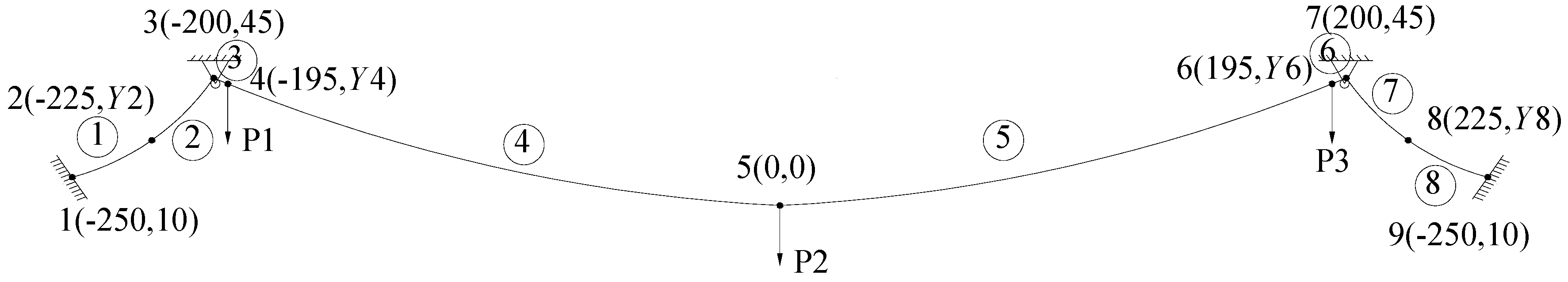
To illustrate the advantages of this method, a three-span suspension bridge with a main span of 400m is chosen as an example, the coordinates of two theoretical vertex positions are (−200, 45) and (200, 45), the coordinate at center of main span is (0, 0), while the coordinates at both ends of side span are (−250, 10) and (250, 10), respectively. The area of cable cross section is 0.5 m², and the elastic modulus is 2.0 × 10⁵ MPa, the equivalent density is 77 kN/m³. Calculate the unstressed cable length, internal forces, and other coordinates of the main cable system under two load cases, as shown in Figure 2:

Load case 1: P₁ = 3000 kN, P₂ = 3500 kN, P₃ = 3000 kN;

Load case 2: P₁ = 2.0 × 10⁵ kN, P₂ = 0 kN, P₃ = 0 kN.

The main cable system is calculated while using the traditional (without introduction of search algorithms) and the improved numerical analysis method. The calculation results are almost the same under load case 1, as shown in

Table 1. Results of y-coordinate under two load cases (unit: m).

Item	Load Case 1				Load Case 2
Node No.	2	4	6	8	2	4	6	8
x	−225.0000	−195.0000	195.0000	225.0000	−225.0000	−195.0000	195.0000	225.0000
y	26.9209	42.5396	42.5396	26.9209	26.9795	9.1986	43.1848	26.9795

and

Table 2. Results of the length and tension force of each cable element under load case 1.

Element No.	Unstressed Cable Length/m	Shape Length/m	Force at Left End/kN		Force at Right End/kN
			Horizontal Component	Vertical Component	Horizontal Component	Vertical Component
①	30.1798	30.1893	−0.2585 × 105	−0.1690 × 105	0.2585 × 105	0.1809 × 105
②	30.8435	30.8527	−0.2585 × 105	−0.1809 × 105	0.2585 × 105	0.1930 × 105
③	5.5709	5.5720	−0.2585 × 105	0.1283 × 105	0.2585 × 105	−0.1261 × 105
④	200.2295	200.2827	−0.2585 × 105	0.9609 × 104	0.2585 × 105	−0.1750 × 104
⑤	200.2295	200.2827	−0.2585 × 105	−0.1750 × 104	0.2585 × 105	0.9609 × 104
⑥	5.5709	5.5720	−0.2585 × 105	−0.1261 × 105	0.2585 × 105	0.1283 × 105
⑦	30.8435	30.8527	−0.2585 × 105	0.1930 × 105	0.2585 × 105	−0.1809 × 105
⑧	30.1798	30.1893	−0.2585 × 105	0.1809 × 105	0.2585 × 105	−0.1690 × 105

; however, under load case 2, there was no solution using traditional numerical analysis method, the calculation results by improved numerical analysis method were shown in Table 1 and

Table 3. Results of the length and tension force of each cable element under load case 2.

Element No.	Unstressed Cable Length/m	Shape Length/m	Force at Left End/kN		Force at Right End/kN
			Horizontal Component	Vertical Component	Horizontal Component	Vertical Component
①	30.2114	30.2219	−0.2876 × 105	−0.1894 × 105	0.2876 × 105	0.2013 × 105
②	30.8072	30.8171	−0.2876 × 105	−0.2013 × 105	0.2876 × 105	0.2134 × 105
③	36.0732	36.1472	−0.2876 × 105	0.2066 × 106	0.2876 × 105	−0.2052 × 106
④	195.7354	195.7919	−0.2876 × 105	0.5206 × 104	0.2876 × 105	0.2477 × 104
⑤	200.2276	200.2867	−0.2876 × 105	−0.2477 × 104	0.2876 × 105	0.1034 × 105
⑥	5.3176	5.3188	−0.2876 × 105	−0.1034 × 105	0.2876 × 105	0.1054 × 105
⑦	30.8078	30.8182	−0.2876 × 105	0.2134× 105	0.2876 × 105	−0.2013 × 105
⑧	30.2114	30.2219	−0.2876 × 105	0.2013 × 105	0.2876 × 105	−0.1894 × 105

.

4.2. Example 2

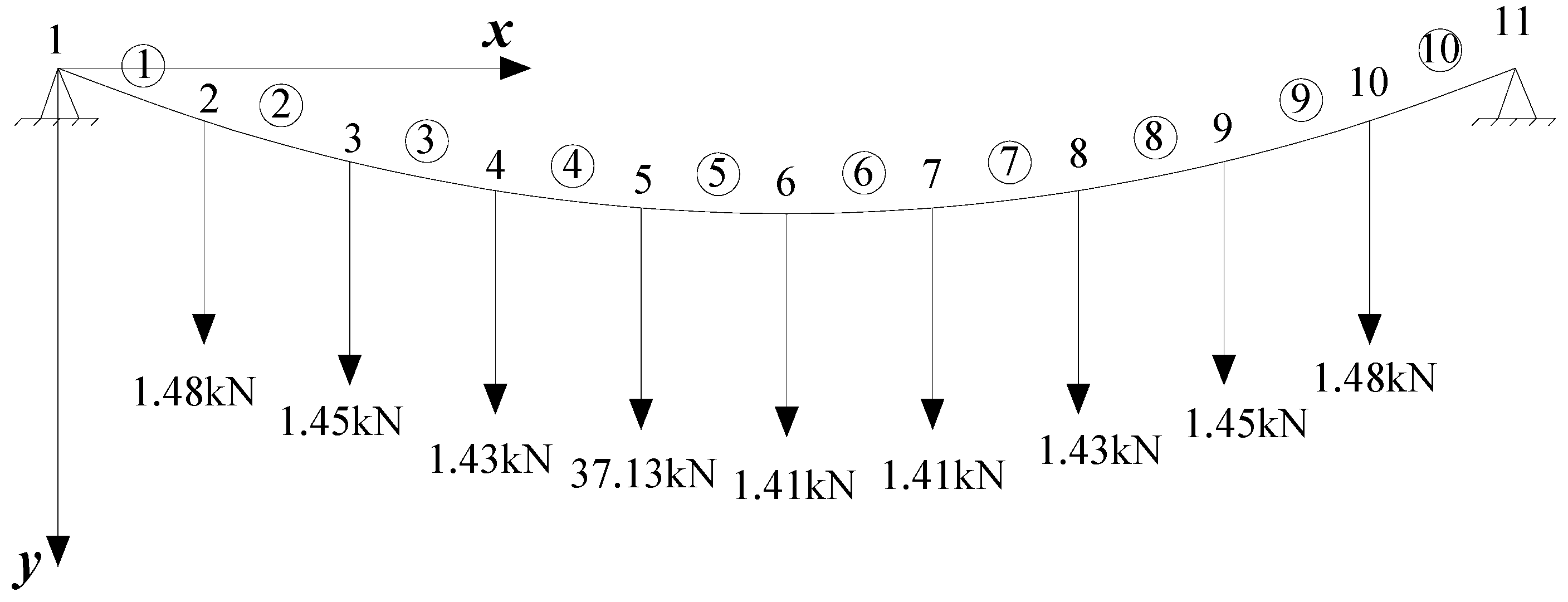
A single span flexible cable that is fixed at both ends subjected to multiple concentrated loads is adopted as an example, as shown in Figure 3, to compare the analytical results from the proposed algorithm with that from other methods. The node coordinates and unstressed lengths of cable segments at initial state are shown in

Table 4. Node coordinates of cable segments at initial state (unit: m).

Node	1	2	3	4	5	6	7	8	9	10	11
x	0.0	30.48	60.96	91.44	121.92	152.40	182.88	213.36	243.84	274.32	304.80
y	0.0	−11.0642	−19.5986	−25.6565	−29.2760	−30.4800	−29.2760	−25.6565	−19.5986	−11.0642	0.0

and

Table 5. Node coordinates of cable segments at initial state (unit: m).

Element	①	②	③	④	⑤	⑥	⑦	⑧	⑨	⑩
Unstressed Length	32.4175	31.6441	31.0683	30.6865	30.4962	30.4962	30.6865	31.0683	31.6441	32.4175

, respectively. In addition, the cross-sectional area of cable is 5.48386 × 10⁻⁴ m², and the elastic modulus is 13,1473.43 MPa, the weight of unit length cable is 47.02594 kN/m.

The configuration and tension force of cable at the equilibrium state under applied load were calculated by different methods, including method 1: improved analytical algorithm in present study; method 2: finite element method in Ref. [41]; and, method 3: traditional analytical method in Ref. [42]. The segmental catenary theory is adopted for both method 1 and 3, however, method 1 uses the search algorithm with penalty factor, while method 3 uses traditional Newton-Raphson iteration algorithm. The comparison of cable configuration and internal forces are shown in

Table 6. Node coordinates of cable segments under applied load (unit: m).

Node	x			y
	Method 1	Method 2	Method 3	Method 1	Method 2	Method 3
1	0.000	0.000	0.000	0.000	0.000	0.000
2	30.995	30.996	30.995	−9.641	−9.638	−9.640
3	61.389	61.391	61.389	−18.595	−18.589	−18.595
4	91.357	91.356	91.357	−26.942	−26.945	−26.942
5	121.075	121.075	121.075	−34.748	−34.748	−34.748
6	151.276	151.276	151.276	−30.242	−30.243	−30.242
7	181.404	181.404	181.404	−25.275	−25.277	−25.275
8	211.641	211.641	211.641	−19.818	−19.817	−19.818
9	242.166	242.166	242.166	−13.825	−13.824	−13.825
10	273.159	273.159	273.159	−7.241	−7.240	−7.241
11	304.800	304.800	304.800	0.000	0.000	0.000

and

Table 7. Tension force of cable segments under applied load (unit: kN).

Element	Tension Force
	Method 1	Method 2	Method 3
①	94.41	94.40	94.40
②	93.98	94.00	94.00
③	93.58	93.60	93.70
④	93.21	93.20	93.30
⑤	91.15	91.20	91.20
⑥	91.37	91.40	91.40
⑦	91.61	91.60	91.70
⑧	91.87	91.90	91.90
⑨	92.16	92.20	92.20
⑩	92.48	92.50	92.50

, respectively. It can be found that the note coordinates and tension force of cable under applied load calculated from improved analytical algorithm agree well with that from method 2 and 3, the maximum difference of node coordinate between method 1 and 2 is 6 mm (y of node 3) with relative error of 0.03%, and 1 mm (y of node 2) between method 1 and 3 with relative error of 0.01%; the maximum difference of the cable tension force between method 1 and 2 is 0.05 kN (element 5) with a relative error of 0.06%, and 0.12 kN (element 3) between method 1 and 3 with relative error of 0.1%. In compression of method 2, the initial node coordinates of cable segments are not necessary for the proposed algorithm to calculate the configuration and tension force of cable at equilibrium state. In comparison to method 3, the initial value is not sensitive to solve cable segment equations for the proposed algorithm especially under the conditions of asymmetric and uneven loads, and also the number of iterations is significantly reduced, resulting in faster convergence speed.

5. Conclusions

(1)

It is theoretically proved that there is no solution for calculating the main cable system in main span or side span under certain loading conditions.

(2)

By introducing the search algorithm and penalty factor, a numerical analysis method was improved to overcome the problem of no solution under certain loading conditions, and to develop the segmental catenary theory.

(3)

The necessity and effectiveness of the improved analytical method were described by the theoretical calculation results and numerical examples. The program using proposed method has been successfully applied in shape finding during design and configuration control during construction of main cable system for suspension bridges in China.

References

- Pugsley, A. The Theory of Suspension Bridges, 2nd ed.; Arnold Ltd.: London, UK, 1968. [Google Scholar]
- Gimsing, N.J.; Georgakis, C.T. Cable Supported Bridges: Concept and Design, 3rd ed.; Wiley: New York, NY, USA, 2012. [Google Scholar]
- Clemente, P.; Nicolosi, G.; Raithel, A. Preliminary design of very long-span suspension bridges. Eng. Struct. 2000, 22, 1699–1706. [Google Scholar] [CrossRef]
- Hong, N.-K.; Koh, H.-M.; Hong, S.-G. Conceptual Design of Suspension Bridges: From Concept to Simulation. J. Comput. Civ. Eng. 2016, 30, 04015068. [Google Scholar] [CrossRef]
- Papavasileiou, G.S.; Pnevmatikos, N.G. Optimized design of steel buildings against earthquake and progressive collapse using cables. Int. J. Progress Sci. Technol. 2017, 6, 213–220. [Google Scholar]
- Hanaor, A. Prestressed pin-jointed structures-flexibility analysis and prestress design. Comput. Struct. 1988, 28, 757–769. [Google Scholar] [CrossRef]
- Murakami, H. Static and dynamic analyses of tensegrity structures. Part II. Quasi-static analysis. Int. J. Solids Struct. 2001, 38, 3615–3629. [Google Scholar] [CrossRef]
- Motro, R. Tensegrity systems and geodesic domes. Int. J. Space Struct. 1990, 5, 341–351. [Google Scholar] [CrossRef]
- Kim, K.-S.; Lee, H.S. Analysis of target configurations under dead loads for cable-supported bridges. Comput. Struct. 2001, 79, 2681–2692. [Google Scholar] [CrossRef]
- Kim, H.-K.; Lee, M.-J.; Chang, S.-P. Non-linear shape-finding analysis of a self-anchored suspension bridge. Eng. Struct. 2002, 24, 1547–1559. [Google Scholar] [CrossRef]
- Sun, Y.; Zhu, H.-P.; Xu, D. New Method for Shape Finding of Self-Anchored Suspension Bridges with Three-Dimensionally Curved Cables. J. Bridg. Eng. 2015, 20, 04014063. [Google Scholar] [CrossRef]
- Karoumi, R. Some modeling aspects in the nonlinear finite element analysis of cable supported bridges. Comput. Struct. 1999, 71, 397–412. [Google Scholar] [CrossRef]
- Wang, P.-H.; Lin, H.-T.; Tang, T.-Y. Study on nonlinear analysis of a highly redundant cable-stayed bridge. Comput. Struct. 2002, 80, 165–182. [Google Scholar] [CrossRef]
- Tang, M.L.; Qiang, S.Z.; Shen, R.L. Segmental catenary method of calculating the cable curve of suspension bridge. J. China Railw. Soc. 2003, 25, 87–91. (In Chinese) [Google Scholar]
- Luo, X.H. Numerical analysis method for cable system of suspension bridges. J. Tongji Univ. (Nat. Sci.) 2004, 32, 441–445. (In Chinese) [Google Scholar]
- Takagi, R.; Nakamura, T.; Nakagawa, K. A new design technique for pre-stressed loads of a cable-stayed bridge. Comput. Struct. 1995, 58, 607–612. [Google Scholar] [CrossRef]
- Lonetti, P.; Pascuzzo, A. Optimum design analysis of hybrid cable-stayed suspension bridges. Adv. Eng. Softw. 2014, 73, 53–66. [Google Scholar] [CrossRef]
- Kim, H.-K.; Kim, M.-Y. Efficient combination of a TCUD method and an initial force method for determining initial shapes of cable-supported bridges. Int. J. Steel Struct. 2012, 12, 157–174. [Google Scholar] [CrossRef]
- Chen, Z.; Cao, H.; Zhu, H.; Hu, J.; Li, S. A simplified structural mechanics model for cable-truss footbridges and its implications for preliminary design. Eng. Struct. 2014, 68, 121–133. [Google Scholar] [CrossRef]
- Ernst, H.J. Der E-modul von seilenunterberucksichtigung des durchhanges. Der Bauing. 1965, 40, 52–55. [Google Scholar]
- Chu, K.H.; Ma, C.C. Nonlinear cable and frame interaction. J. Struct. Div. ASCE 1976, 102, 569–589. [Google Scholar]
- Nazmy, A.S.; Abdel-Ghaffar, A.M. Three dimensional nonlinear static analysis of cable-stayed bridges. Comput. Struct. 1990, 34, 257–271. [Google Scholar] [CrossRef]
- Ren, W.-X.; Huang, M.-G.; Hu, W.-H. A parabolic cable element for static analysis of cable structures. Eng. Comput. 2008, 25, 366–384. [Google Scholar] [CrossRef]
- Tang, J.M.; Dong, M.; Qian, R.J. A finite element method with five-node isoparametric element for nonlinear analysis of tension structures. Chin. J. Comput. Mech. 1997, 14, 108–113. (In Chinese) [Google Scholar]
- Ni, Y.Q.; Ko, J.M.; Zheng, G. Dynamic analysis of large-diameter sagged cables taking in account flexural rigidity. J. Sound Vib. 2002, 257, 301–319. [Google Scholar] [CrossRef]
- Ren, W.X.; Harik, I.E.; Blandford, G.E. Roebling suspension bridge: I. FE model and free vibration response. J. Bridg. Eng. ASCE 2004, 9, 119–126. [Google Scholar] [CrossRef]
- Ozdemir, H. A finite element approach for cable problems. Int. J. Solids Struct. 1979, 15, 427–437. [Google Scholar] [CrossRef]
- Liew, J.; Punniyakotty, N.; Shanmugam, N. Limit-state analysis and design of cable-tensioned structures. Int. J. Space Struct. 2001, 16, 95–110. [Google Scholar] [CrossRef]
- Ali, H.; Abdel-Ghaffar, A. Modeling the nonlinear seismic behavior of cable-stayed bridges with passive control bearings. Comput. Struct. 1995, 54, 461–492. [Google Scholar] [CrossRef]
- Chen, Z.H.; Wu, Y.J.; Yin, Y.; Shan, C. Formulation and application of multi-node sliding cable element for the analysis of Suspend-Dome structures. Finite Elem. Anal. Des. 2010, 46, 743–750. [Google Scholar] [CrossRef]
- O’Brien, W.; Francis, A. Cable movements under two-dimensional loads. J. Struct. Div. ASCE 1964, 90, 89–123. [Google Scholar]
- Jayaraman, H.; Knudson, W. A curved element for the analysis of cable structures. Comput. Struct. 1981, 14, 325–333. [Google Scholar] [CrossRef]
- Irvine, H.M. Cable Structures; The MIT Press: Cambridge, UK, 1981. [Google Scholar]
- Wang, C.; Wang, R.; Dong, S.; Qian, R. A new catenary cable element. Int. J. Space Struct. 2003, 18, 269–275. [Google Scholar]
- Yang, Y.B.; Tsay, J.Y. Geometric nonlinear analysis of cable structures with a two-node cable element by generalized displacement control method. Int. J. Struct. Stab. Dyn. 2007, 7, 571–588. [Google Scholar] [CrossRef]
- Such, M.; Jimenez-Octavio, J.R.; Carnicero, A.; Lopez-Garcia, O. An approach based on the catenary equation to deal with static analysis of three dimensional cable structures. Eng. Struct. 2009, 31, 2162–2170. [Google Scholar] [CrossRef]
- Li, C. Refined Calculation Theory for Nonlinear Analysis of Suspension Bridge with Composite Beam. Ph.D. Dissertation, Hunan University, Changsha, China, 2006. (In Chinese). [Google Scholar]
- Li, C.; Ke, H.; Liu, J.; Dong, C. Key technologies of construction control system transformation for pingsheng bridge. China Civ. Eng. J. 2008, 41, 49–54. (In Chinese) [Google Scholar]
- Ke, H.; Li, C.; Zhang, Y.; Dong, C. System transformation program and control principles of suspender for a self-anchored suspension bridge with two towers and large transverse inclination spatial cables. China Civ. Eng. J. 2008, 43, 94–101. (In Chinese) [Google Scholar]
- Li, C.; Ke, H.; Yang, W.; He, J.; Li, H. Comparative study on optimal system transformation schemes for Taohuyu self-anchored suspension bridge. China Civ. Eng. J. 2014, 47, 120–127. (In Chinese) [Google Scholar]
- Saffan, S.A. Theoretical analysis of suspension bridges. Proc. ASCE 1966, 92, 1–11. [Google Scholar]
- Tang, M. 3D Geometric Nonlinear Analysis of Long-Span Suspension Bridge and Its software Development. Ph.D. Dissertation, Southwest Jiaotong University, Chengdu, China, 2003. (In Chinese). [Google Scholar]
Figure 1.
An elastic catenary cable segment.
Figure 2.
A three-span suspension cable system.
Figure 3.
A single span cable subjected to multiple concentrated loads.