Acoustic Wave Propagation in Air-Filled Pipes Using Finite Element Analysis

Abstract

The major objective of this work is to develop an efficient Finite Element Analysis (FEA) procedure to simulate wave propagation in air-filled pipes accurately. The development of such a simulation technique is essential in the study of wave propagation in pipe networks such as oil and gas pipelines and urban water distribution networks. While numerical analysis using FEA seems superficially straight forward, this paper demonstrates that the element type and refinement used for acoustic FEA have a significant effect on the accuracy of the result achieved and the efficiency of the computation. In particular, it is shown that the well-known, better overall performance achieved with 3D solid hexahedral elements in comparison with 2D-type elements in most stress and thermal applications does not occur with acoustic analysis. In this paper, FEA models were developed taking into account the influence of element type and sizes using 2D-like and 3D element formulations, as well as linear and quadratic nodal interpolations. Different mesh sizes, ranging from large to very small acoustic wavelengths, were considered. The simulation scheme was verified using the Time of Flight approach to derive the predicted acoustic wave velocity which was compared with the true acoustic wave velocity, based on the input bulk modulus and density of air. For finite element sizes of the same order as acoustic wavelengths which correspond to acoustic frequencies between 1 kHz and 1 MHz, the errors associated with the predictions based on the 3D solid hexahedral acoustic elements were mostly greater than 15%. However, for the same element sizes, the errors associated with the predictions based on the 2D-like axisymmetric solid acoustic elements were mostly less than 2%. This indicates that the 2D-like axisymmetric solid acoustic elements are much more efficient than the 3D hexahedral acoustic elements in predicting acoustic wave propagation in air-filled pipes, as they give higher accuracies and are less computationally intensive. In most stress and thermal FEA, the 3D solid hexahedral elements are much more efficient than 2D-type elements. However, for acoustic FEA, the results show that 2D-like axisymmetric elements are much more efficient than 3D solid hexahedral elements.

1. Introduction

Understanding the wave propagation in a pipe is of fundamental importance to some engineering systems such as oil and gas pipeline systems and urban water distribution networks. Pipelines are extensively used to transport energy products like crude oil and gas, and for water transport and distribution. Corrosion flaws can begin to develop as pipelines age, and it is therefore vital to develop ways to inspect them efficiently. Many industrial pipelines are buried in the ground and are mostly isolated and inaccessible. Therefore, there is a need to employ remote sensing techniques to monitor the development of flaws in such pipelines. The acoustic wave propagation technique has become a very attractive, non-destructive testing technique for the remote monitoring of pipelines. The wave propagation technique has the advantage of full volumetric inspection, and can be used to find the characteristics of flow in a fluid-filled pipeline. The acoustic wave propagation technique operates in elongated geometrical bodies with constant or variable cross-sections, e.g., pipes. Sound generated in these bodies is constrained to propagate in the pipe wall, as well as in the fluid inside the pipe, and is reflected back to the generation point when a change in impedance (discontinuity) occurs. Therefore, acoustic wave propagation can only occur when there is a medium in which to propagate.

Acoustic wave propagation phenomena along pipelines have been investigated theoretically and experimentally. Several modifications of the acoustic wave equation to more complex equations have been established. For instance, for a fluid flowing with varying density and acoustic velocity, Bergmann [1] previously proposed an equation that is widely used in underwater acoustics problems, whereas Pierce [2] derived a generalized wave equation for an inhomogeneous fluid in motion whose flow profile differs in time and position. Chen and Shen [3] proposed a method to analyze the surface waves propagating on a grounded anisotropic slab. They considered the field variation in the direction parallel to the wave propagation. The wave propagation characteristics were derived on the basis of Maxwell’s equation and boundary conditions.

Recent developments showed that acoustic wave propagation using the Finite Element Method (FEM) has been utilized in pipeline detection. The sound propagation within a fluid flow in a pipe can be evaluated, taking the flow profile as a boundary condition for the simulation task. The FEA solvers for linear and non-linear acoustic wave equations vary. This leads to a symmetric matrix formulation for fluid-structure interaction [4], and this is being used in several computation solvers for acoustics. Mohamed and Walied [5] developed a finite element model of a surface acoustic wave sensor using the ANSYS simulation tool; the model was tested for hydrogen detection. Another numerical FEA approach was proposed for the calculation of non-linear propagation of acoustic waves by Kagawa et al. [6].

Eccardt et al. [7] presented an FEA method based on a modified wave equation, and compared their results with previously developed techniques like the Holtz-Kirchhoff integral and ray tracing method. They obtained sets of primary and secondary wave equations, and for numerical implementation, they employed the Finite Element Method to discretize and solve the equation integral scheme with respect to time. The numerical result shows that the equations are valid, but with more pronounced discretization error for the secondary waves. An FE numerical technique for simulating a 3D acoustic-wave correlator was presented by Tikka et al. [8]. They presented and discussed the results of the analysis of device responses for variable acoustic modes and differences in electrical response in the system. They concluded that FEA provides an effective means of analysing the correlator’s response to various propagating modes.

Kutiš et al. [9] used FEM in modelling and simulation of surface acoustic wave sensor. They performed modal and transient piezoelectric analysis to determine the eigenmodes and frequencies of the system that were used to investigate the harmonic wave propagation characteristics of the system. Yu and Yan [10] conducted a series of numerical studies using FEA to investigate the wave propagation behaviour in wooden poles. Their results showed that a higher elastic modulus in longitudinal direction always generated higher guided wave behaviour in a wooden pole, and experimental testing was performed to validate their findings. Many works have been conducted with the aim of improving the computational efficiency and accuracy of the convectional FEA method. Owowo and Oyadiji [11] investigated the effect of leakage on acoustic wave propagation in an air-filled pipe using the FEA method and experimental testing. Their predicted and measured data was subsequently used to identify and locate the leakage using a Time-of-Flight approach.

Other numerical techniques have been used for predicting acoustic wave propagation. These include the Boundary Element Method (BEM), Statistical Energy Analysis (SEA), and the SWAN (Simulating Waves Nearshore) spectral phase averaged wave model. For example, Chen et al. [12] used the Finite Element Method and Boundary Element Method (FEM-BEM) to analyse acoustic fluid-structure interaction. An algorithm based on FEM-BEM was presented for simulation of fluid-structure interaction in their work. The accuracy of the simulation was improved by evaluating the single integrals in boundary integral equations using the Cauchy principal value and the Hadamard finite part integral method.

In order to understand the mechanism of acoustic wave propagation in a body, the noise propagation in ship structures was investigated by Weryk et al. [13], and was tested in several vessels using Statistic Energy Analysis (SEA). Their predicted result was compared with the experimental results obtained from tests carried out using similar vessels. Eugen [14] studied the patterns by which wave energy propagates in the western side of the Black sea and simulated the propagation using the SWAN spectral phase averaged wave model. The study shows that there is a tendency for the waves to travel faster along the Black sea surface.

A field experiment to assess the feasibility of using commercially available accelerometers and related signal condition to analyse acoustic wave propagation in a pipe was recently conducted [15]. Results from the experiments confirmed that attenuation is the most important factor that affects the viability of acoustic wave propagation for impact detection. In another work, a sound intensity measurement technique was used to investigate how sound energy propagates around organ pipes [16]. The authors obtained the sound intensity distributions around the pipes, and the directions of the acoustic energy flow were presented. Papadopoulou et al. [17] used the acoustics pulse reflectometer technique for flaw detection in pipes in the time domain.

The use of analytical equations to investigate acoustic- or pressure-wave propagation in a fluid-filled pipeline might be straight-forward and easily implemented for a simple straight pipe. However, when pipe networks are involved, the prediction of acoustic or pressure wave propagation becomes very difficult to implement analytically. In such cases, the use of a numerical method, such as FEA, is imperative. However, large errors may also occur in the numerical predictions of acoustic wave propagation. For example, when FEA was used to predict acoustic wave propagation in an air-filled pipe, as in the work by Owowo and Oyadiji [11], very large acoustic speed errors were obtained. They used 3D hexahedral acoustic elements whose structural counterparts usually give accurate predictions. They expected the 3D hexahedral acoustic elements to also give accurate predictions, but did not check to confirm the degree of their accuracy. Therefore, there is a need to further investigate the FEA of acoustic wave propagation in fluid-filled pipes using other acoustic finite elements in order to achieve accurate and efficient predictions.

In this paper, the simulation of acoustic wave propagation in a pipe using FEA is presented and verified using the Time of Flight approach to deduce the acoustic velocity associated with the predictions. The use of different acoustic element types of 2D-like and 3D formulations, and of linear and quadratic interpolations, are investigated in order to deduce the most accurate acoustic FEA approach, and thereby, to minimise the errors.

2. Acoustic Wave Theory and Finite Element Formulation

2.1. Acoustic Wave Theory

Acoustic wave propagation in a homogenous fluid media at rest is governed by the wave equation:

$${𝞩}^2\Phi =\frac{1}{{\mathrm{c}}^2}\frac{{\partial }^2\Phi }{\partial t^2}$$

(1)

For Cartesian and polar coordinates, (x, y, z) and (r, θ, z), respectively, the three-dimensional Laplacian operator $𝞩$ is defined, respectively by:

$${𝞩}^2=\frac{{\partial }^2}{\partial x^2}+\frac{{\partial }^2}{\partial y^2}+\frac{{\partial }^2}{\partial z^2}$$

(2)

and

$${𝞩}^2=\frac{{\partial }^2}{\partial r^2}+\frac{1}{r}\frac{{\partial }^2}{\partial r^2}+\frac{1}{r^2}\frac{{\partial }^2}{\partial {\theta }^2}+\frac{{\partial }^2}{\partial z^2}$$

(3)

and the equations for coordinate transformations are given by:

$$x=rcos\theta ,y=rsin\theta ,r=\sqrt{x^2+y^2}$$

(4)

where c is the velocity of acoustic wave propagation, Φ velocity potential and x, y, and z are standard Cartesian coordinates. The corresponding acoustic pressure wave propagation is governed by:

$${𝞩}^{2}p=\frac{1}{c^2}\frac{{\partial }^{2}p}{\partial t^2}$$

(5)

where the pressure, p and instantaneous particle velocity, u are related to the velocity potential, Φ by:

$$u=𝞩\Phi ;p=-\rho \frac{\partial \Phi }{\partial t}$$

(6)

For an open-ended air-filled pipe without defect, with uniform cross-sectional area, driven by a sound pulse, the general solution of Equation (1) is of the form [18]:

$$q_{k_x,k_y,k_z}\left(x,y,z,t\right)=A{e}^{i\left(k_{x}x+k_{y}y+k_{z}z-\omega t\right)}$$

(7)

or

$$q_{k_r,k_{\theta },k_z}\left(r,\theta ,z,t\right)=A{e}^{i\left(k_{r}r+k_{\theta }\theta +k_{z}z-\omega t\right)}$$

(8)

where q represents the longitudinal displacement of the fluid as the wave propagates through it, t is time, $\omega$ is the frequency and k is the wave number. The FEA method based on Equation (1) leads to a symmetric matrix formulation for fluid structure interaction [1,3] which is used in several numerical computational analysis programs for acoustics. For direct integration transient analysis, FEA solutions are based on Equation (7).

2.2. Acoustic Finite Element Formulation in the Abaqus FEA Software

The acoustic elements in the Abaqus FEA software model the propagation of acoustic waves, and are active in dynamic analysis procedures. In the Abaqus FEA software (version 6.14, ABAQUS Inc, Johnston, RI, USA), the analysis with acoustic elements should be thought of as small-displacement linear perturbation analysis. The equation for small motions of compressible, adiabatic fluid is taken to be [19]:

$$\frac{\partial p}{\partial x}+\gamma \dot{u}\left(x,\alpha \right)+\rho \ddot{u}\left(x,\alpha \right)=0$$

(9)

where p is the pressure in the fluid, $x$ is the spatial position of the fluid particle, $\dot{u}$ is the fluid particle velocity, $\ddot{u}$ is the fluid particle acceleration, $\rho$ is the density of the fluid, $\gamma$ is the “volumetric drag” (force per unit volume per velocity), and $\alpha$ are independent field variables such as temperature, humidity of air, or salinity of water, on which $\rho$ and $\gamma$ may depend.

The constitutive behavior of the fluid is assumed to be inviscid, linear, and compressible; the pressure can be obtained as

$$p=-K\left(x,\alpha \right)\frac{\partial }{\partial x}·u$$

(10)

where $K$ is the bulk modulus of the fluid.

2.3. Direct Integration Transient Dynamics Formulation

The partial differential equation used in direct integration transient analysis in the Abaqus FEA software is obtained by combining Equations (9) and (10), to give the equation of motion for the fluid in terms of the fluid pressure [19]:

$$\frac{1}{K}\ddot{p}+\frac{\gamma }{\rho K}\dot{p}-\frac{\partial }{\partial x}·\left(\frac{1}{\rho }\frac{\partial p}{\partial x}\right)=0$$

(11)

An equivalent weak variational form of the equation of motion, Equation (11), is obtained by introducing an arbitrary variational field, $\delta p$ and integrating over the fluid domain to give:

$${{\displaystyle \int }}_V\delta p\left(\frac{1}{K}\ddot{p}+\frac{\gamma }{\rho K}\dot{p}-\frac{\partial }{\partial x}·\left(\frac{1}{\rho }\frac{\partial p}{\partial x}\right)\right)dV=0$$

(12)

Applying all necessary boundary conditions, Green’s theorem allows the Equation (12) to give the final variational statement for the acoustic medium as [19]:

$${{\displaystyle \int }}_V[\delta p\left(\frac{1}{K}\ddot{p}+\frac{\gamma }{\rho K}\dot{p}\right)+\frac{1}{\rho }\frac{\partial \partial p}{\partial x}·\frac{\partial p}{\partial x}]dV-{{\displaystyle \int }}_s\partial pTdS+{{\displaystyle \int }}_s\partial p\left(\frac{\gamma }{\rho c}p+\left(\frac{\gamma }{\rho K}+\frac{1}{c}\right)\dot{p}+\frac{1}{K}\ddot{p}\right)dS+{{\displaystyle \int }}_s\partial p\left(\frac{1}{c}\dot{p}+\frac{1}{\beta }p\right)dS-{{\displaystyle \int }}_s\partial p\overline{n}·\ddot{u}dS+{{\displaystyle \int }}_s\partial p\left(\frac{\gamma }{\rho c}p+\left(\frac{\gamma }{\rho K}+\frac{1}{c}\right)\dot{p}+\frac{1}{K}\ddot{p}-\overline{n}·\ddot{u}\right)dS=0$$

(13)

where $\overline{n}=-n$ is the inward normal of the surface. For the structural interface:

$${{\displaystyle \int }}_V\delta \epsilon :\sigma dV+{{\displaystyle \int }}_V\beta \rho \delta u·\dot{u}dV+{{\displaystyle \int }}_V\rho \delta u·\ddot{u}dV+{{\displaystyle \int }}_{V}p\delta u·ndS+{{\displaystyle \int }}_V\delta u·tdS=0$$

(14)

where $\sigma$ is the stress at a point in the structure, p is the pressure acting on the fluid-structural interface, n is the outward normal to the structure, $\rho$ is the density of the material, $\beta$ is the mass proportional damping factor, $\ddot{u}$ is the acceleration of a point in the structure, T is the surface traction applied to the structure, $\delta u$ is a variational displacement field, and $\delta \epsilon$ is the strain variation that is compatible with $\delta u$.

2.4. The Discretized Finite Element Equation

The variational problem for the coupled fields $\mathrm{u}$ and p is defined by Equations (13) and (14). The problem domain is discretized by introducing the following interpolation functions (i) in the fluid: $P=H^P{p}^P$, where H is the interpolation function in the fluid domain and superscript $P=1,2,\dots$ up to the number of pressure nodes; and (ii) in the structure: $u=N^N{u}^N$, where N is the interpolation function in the structural domain and superscript $N=1,2,\dots$ up to the number of displacement degrees of freedom. Using Galerkin method and the Petrov-Galerkin substitution, the discretized coupled variational equation is obtained by adding Equations (13) and (14) to give [19]:

$$-\delta {\widehat{P}}^P\{\left(M_f^{PQ}+M_{fr}^{PQ}\right){\ddot{P}}^Q+\left(C_f^{PQ}+C_{fr}^{PQ}\right){\dot{P}}^Q+\left(K_f^{PQ}+K_{fr}^{PQ}+K_{fi}^{PQ}\right)P^Q-S_{fs}^{PM}\ddot{u}-P_f^P\}+\delta u\{I^N+M^{NM}\ddot{u}+C_{\left(m\right)}^{NM}\dot{u}+{\left[S_{fs}^{QN}\right]}^T{P}^Q-P^N\}=0$$

(15)

where the superscripts P, Q refer to pressure degrees of freedom in the fluid and N, M refer to displacement degrees of freedom in the structure and the bracketed terms are integral expressions of the interpolation functions H and N defined in [19].

3. Acoustic Elements

Acoustic elements are formulated for modelling an acoustic medium undergoing small pressure changes. The solution in the acoustic medium is defined by a single pressure variable. Impedance boundary conditions representing absorbing surfaces or radiation to an infinite exterior are available on the surfaces of these acoustic elements. The major acoustic element types in the Abaqus FEA software are the acoustic 3D hexahedral solid elements (AC3D8 and AC3D20) and acoustic axisymmetric solid elements (ACAX4 and ACAX8).

3.1. Acoustic 3D Solid Elements (AC3D8 and AC3D20)

Three-dimensional elements are defined in the global X, Y, Z space. These elements are used when the geometry and/or the applied loading are too complex for any other element type with fewer spatial dimensions. The solid 3D acoustic elements in the Abaqus FEA software includes the 8-node brick (AC3D8) element that has linear nodal interpolations and the 20-node brick (AC3D20) element which has quadratic nodal interpolation as shown in Figure 1.

3.2. Acoustic Axisymmetric Solid Elements (ACAX4 and ACAX8)

Axisymmetric elements provide for the modelling of bodies of revolution under axially symmetric loading conditions. A body of revolution is generated by revolving a plane cross-section about an axis (the symmetry axis), and is readily described in cylindrical polar coordinates r, z, and θ. There are two main acoustic axisymmetric element types used in the Abaqus FEA software: the 4-node quadrilateral element (ACAX4) with linear nodal interpolation and the 8-node quadrilateral (ACAX8) element with quadratic nodal interpolation. Figure 2 shows a typical reference cross-section and the elements in an axisymmetric solid at θ = 0. These elements are defined as if they are 2D elements, but they are actually solid elements when they are internally revolved in the software as illustrated in Figure 2.

4. Acoustic Finite Element Analysis (AFEA) of Acoustic Wave Propagation in a Straight Pipe

4.1. Finite Element Modelling Description

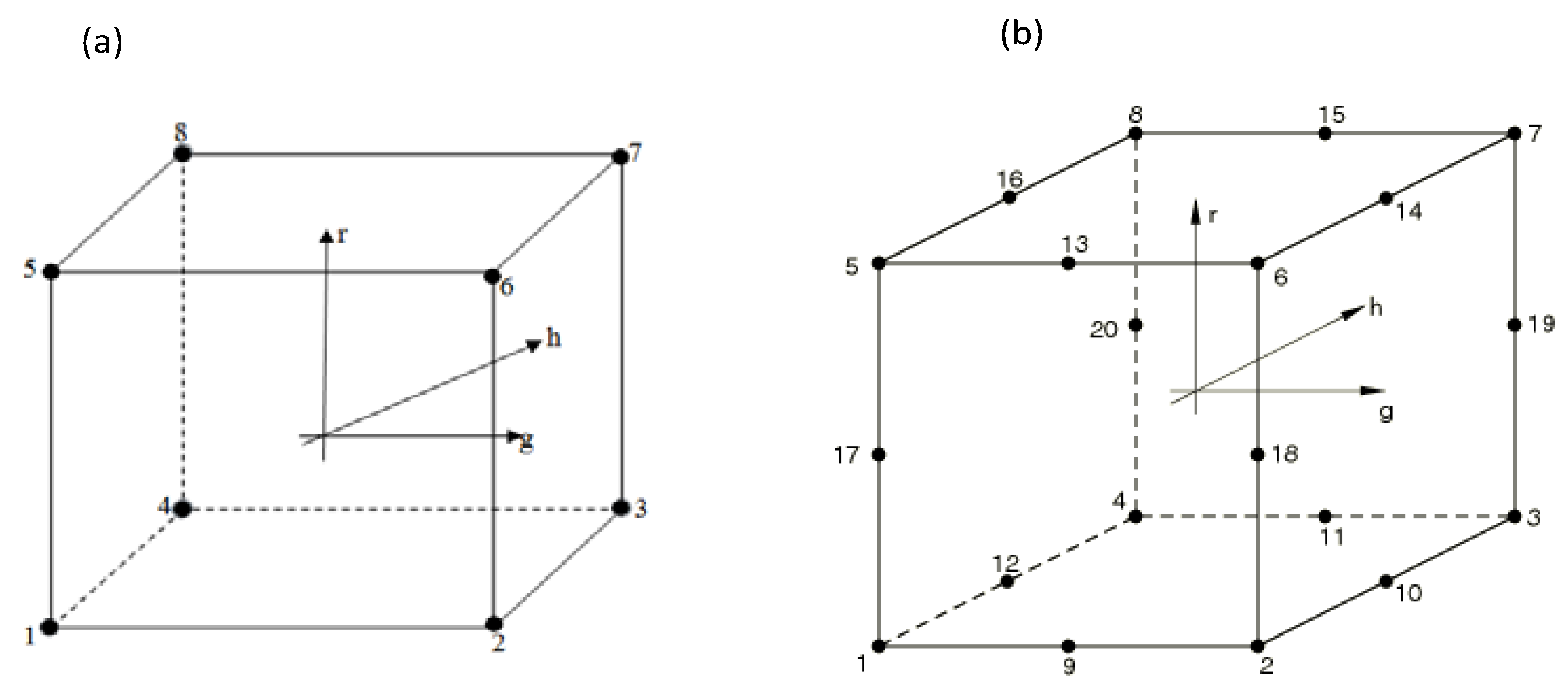
To perform the acoustic wave propagation using FEA in a pipe, three stages must be considered in the numerical modelling: (i) pre-processing, (ii) analysis, and (iii) post-processing. The analysis starts from the development of the geometry of the air cavity (domain) of an air-filled pipe. This is followed by the discretization of the geometry into smaller discrete elements. The elements are joined together by nodes to form a mesh. The amount of elements used for a particular model is referred to as the mesh density. The acoustic finite element is a unique element designed for the simulation of a system undergoing small variation in acoustic pressure. The simulation process of the AFEA of the acoustic wave reflectometry method involves the integration of the geometrical description of a model with the parameters of the fluid-medium, such as: pressure, momentum, and energy across the elements of the domain. The AFEA then evaluates the medium responses at each of the integration points of the elements, thereby obtaining the responses at the nodes that join the elements together.

Thus, for any other point within the elements, results are obtained by interpolation from the nodal data. However, the geometrical order of interpolation is determined by the kind of element employed for the analysis. There are two principal interpolations, namely: linear interpolation used by element types ACAX4 and AC3D8, and quadratic interpolations used by element types ACAX8 and AC3D20 [19].

4.2. Analysis Procedure and Boundary Conditions

In creating the intact pipe model using the solid elements AC3D8 and AC3D20, the 3-D modelling space of the Abaqus/CAE part module was used to create a single solid shape deformable cylinder that represents the model of the air volume that occupied the pipe cavity. In the case of the intact pipe model using the axisymmetric elements ACAX4 and ACAX8, a longitudinal sectional plane of the 3-D modelling space was used to part-define the model from which the full solid shape deformable cylinder was derived internally by revolving the plane about its axis. In both cases, only the fluid (air) content of the pipe was modelled without the inclusion of the pipe in the model. Since the specific acoustic impedance of the air medium is much smaller than the specific impedance of the wall of a metallic or plastic pipe, this assumption is reasonable. This eliminates contact interaction of the solid pipe wall and the fluid, and as a consequence, reduces computational time and resources.

The acoustic properties of air used for the intact models are density $\rho =1.225\mathrm{kg}{\mathrm{m}}^{-3}$ and bulk modulus $ℬ=\mathrm{142,000}\mathrm{N}{\mathrm{m}}^{-2}$ which give an acoustic velocity of $340.47\mathrm{m}{\mathrm{s}}^{-1}$. Volumetric drag of the air medium was assumed to have negligible effect on the analysis and was ignored. The next step in creating the model involves defining and assigning material and section properties to the deformable domain.

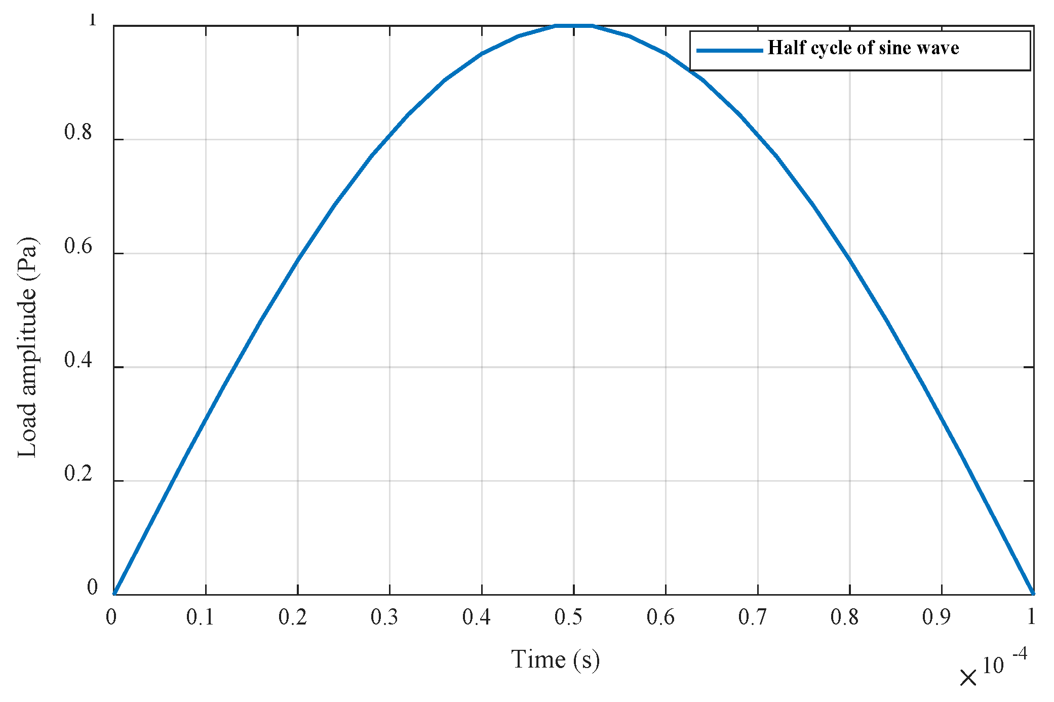
In defining the analysis step for the simulation, the step module of the Abaqus/CAE was selected. The air properties were evaluated to define a general dynamic implicit step with a primary period of $1.469\times {10}^{-3}\mathrm{s}$ for the initial step, and with an increment size set at $1.469\times {10}^{-6}\mathrm{s}$. Also, a fixed maximum number of time increments of $\mathrm{10,000}$ was defined to guarantee convergence in the time increments. The solution technique used for the equation solver was the Full Newton, while the default analysis product that converts severe discontinuity iterations to propagate from the previous step was selected. The extrapolation of prior state of each increment was chosen as linear, while Alpha time integrator parameter was specified as −0.333.

An acoustic impulse of a half sine wave, as shown in Figure 3, was created. The pulse had a maximum amplitude of $1\mathrm{Pa}$, and was applied for a duration of ${10}^{-4}\mathrm{s}$ at the inlet. Similarly, at the pipe outlet region, a zero acoustic pressure was defined to create a profile of pressure damping from maximum to atmospheric at the pipe exit boundary.

4.3. Simulation Results

4.3.1. Verification of Results Using Time of Flight

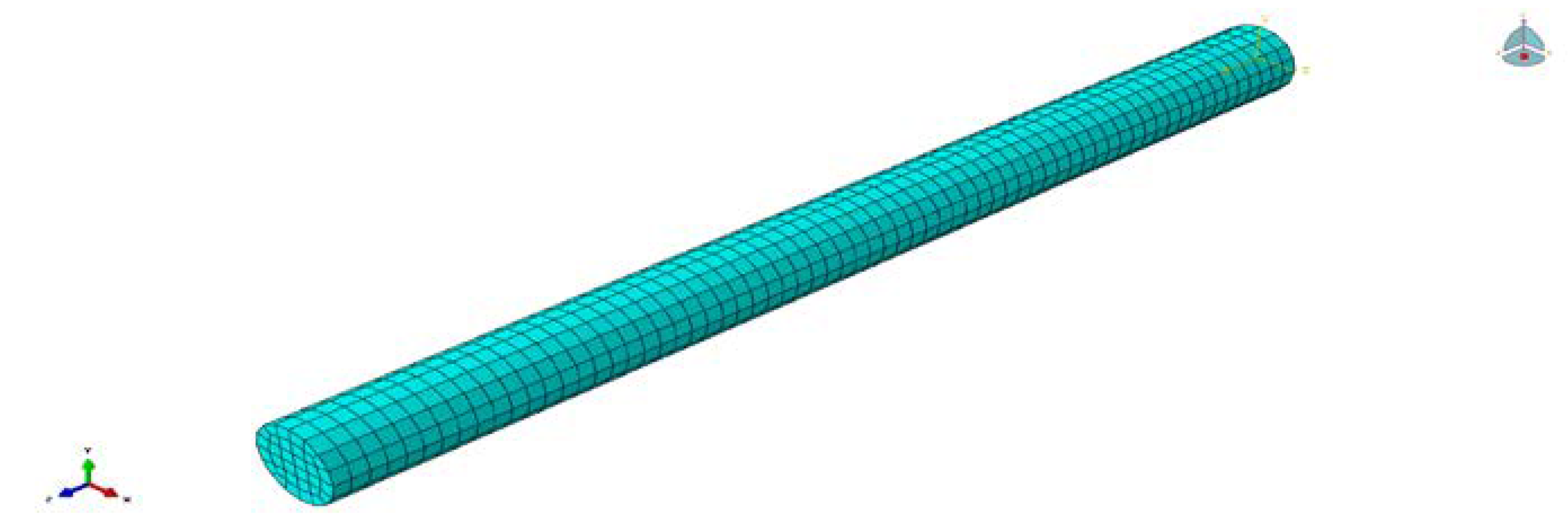
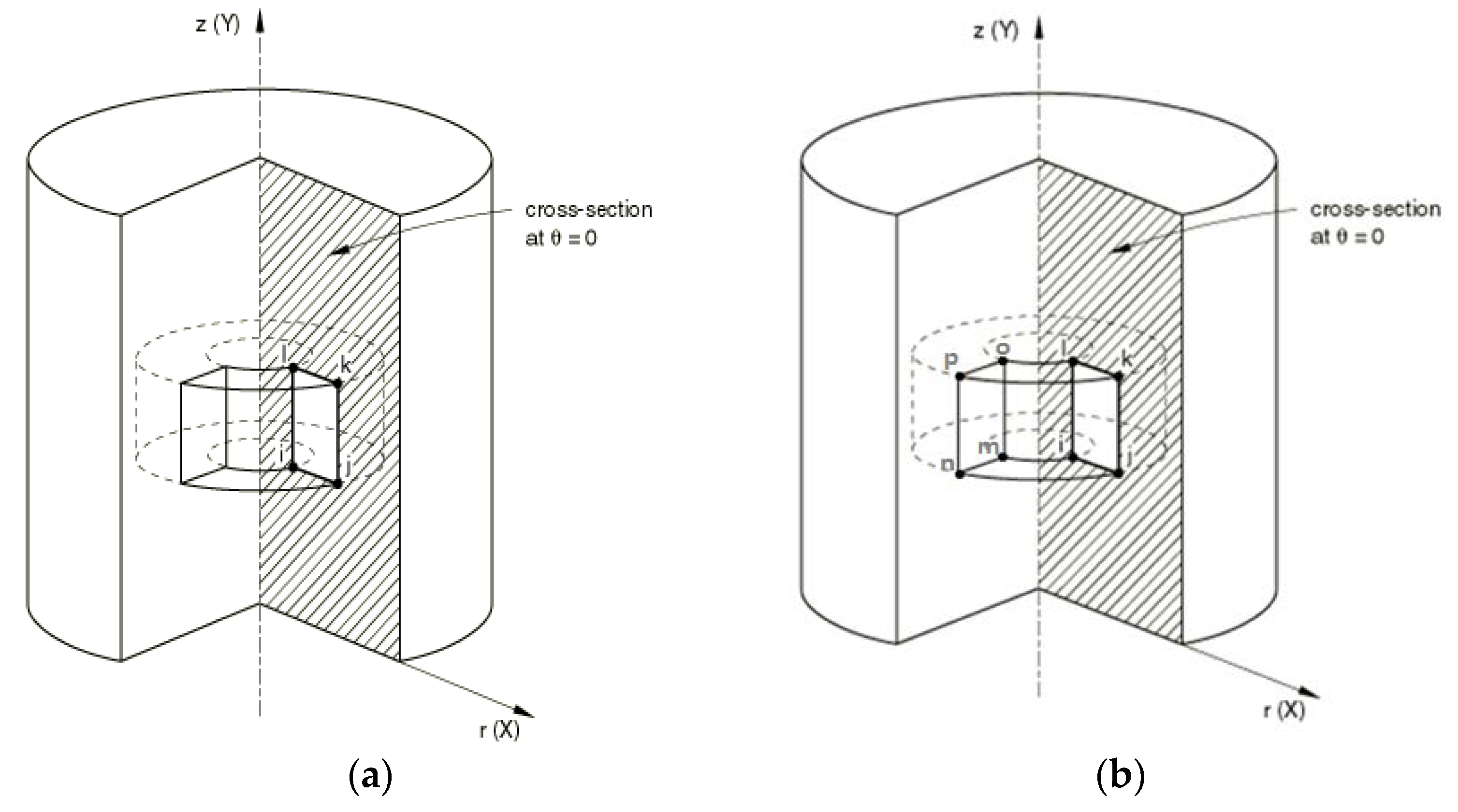
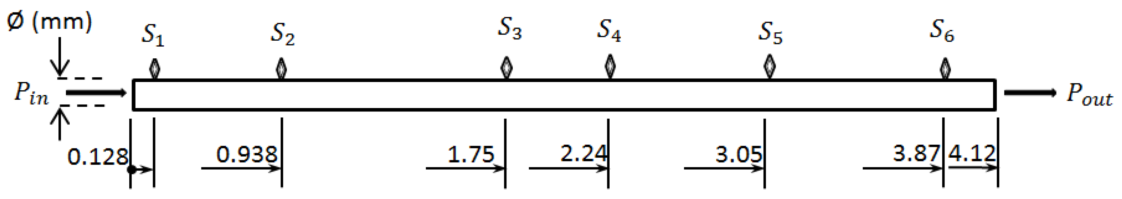
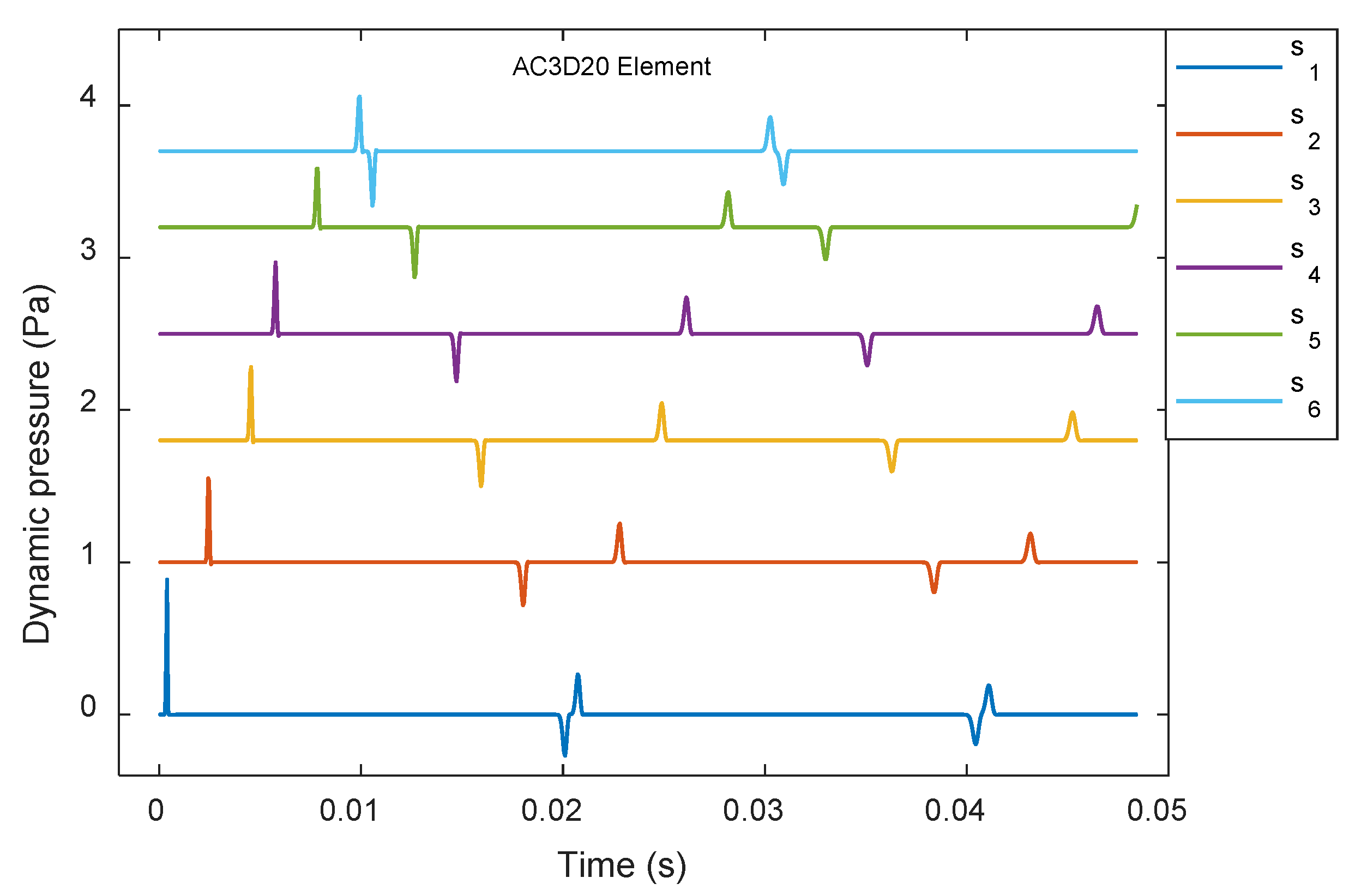
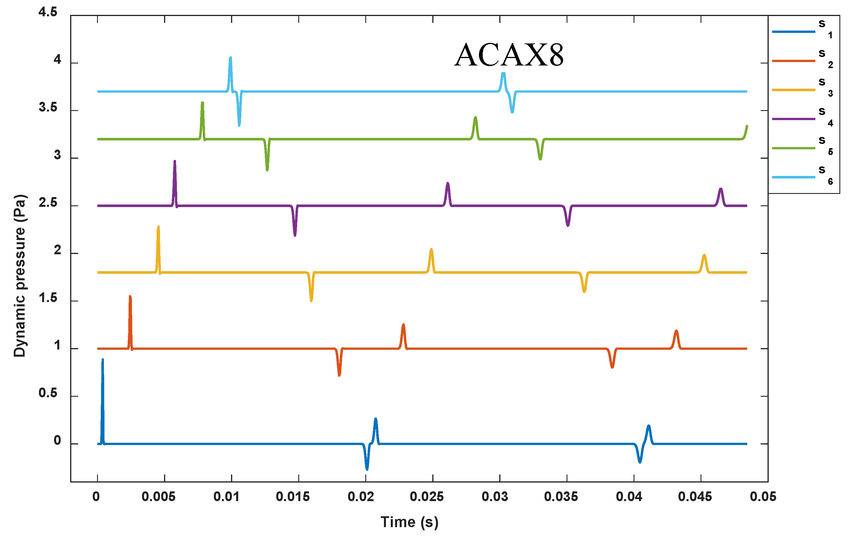
The FEA of acoustic wave propagation in a pipe of diameter $25.4\mathrm{mm}$ and of length 4.02 m was earlier conducted by Owowo and Oyadiji [11]. A 20-node quadratic acoustic brick (AC3D20) element type was employed for their analysis, as illustrated in Figure 4. As a starting point in these investigations, the acoustic wave propagation in the same pipe was analysed using the AC3D20 element type and the same mesh seed size of 9 mm. The responses obtained at six monitoring points, which are designated as ‘sensor’ locations ${\mathrm{s}}_1$ to ${\mathrm{s}}_6$, as shown in Figure 5, are illustrated in Figure 6. These results are identical to those shown in the paper by Owowo and Oyadiji [11], and the Time of Flight approach was used to check their accuracy.

Figure 6 presents stacked plots of the dynamic pressure versus time waveforms at the six monitoring nodes identified in the intact pipe model. It should be noted that all the plots start with a dynamic pressure amplitude of zero. Thus, in all cases, the maximum peak amplitudes are less than 1.0 Pa. The stacking of the plots enables a direct comparison of the forward-going and backward-going (reflected) wavefronts at the different sensor locations. From the figure, the first positive peaks seen in each of the graphs indicate the arrival of the pressure pulse to the individual sensors. The compression pulse propagates past the respective sensors $\left(s_1–s_6\right)$ in the order of time seen in the second column of

Table 1. Arrival Time of Compression and Rarefaction Wave-front using the acoustic continuum 3D 20-node brick elements (AC3D20).

${\mathit{s}}_{\mathit{n}}$	${\mathit{l}}_{\mathit{s}}\mathbf{\left(}\mathbf{m}\mathbf{\right)}$	${\mathit{t}}_{\mathit{s}}\mathbf{\left(}\mathbf{ms}\mathbf{\right)}$	${\mathit{t}}_{\mathit{p}}\mathbf{\left(}\mathbf{ms}\mathbf{\right)}$	$\mathit{c}$$\mathbf{\left(}{\mathbf{ms}}^{\mathbf{-}\mathbf{1}}\mathbf{\right)}$	Error, $\mathbf{E}\mathbf{(}\mathbf{\%}\mathbf{)}$
$s_1$	0.128	0.3	20.5	$395.1$	14.5
$s_2$	0.938	2.2	18.2	$395.4$	14.6
$s_3$	1.758	4.2	16.0	$397.9$	15.3
$s_4$	2.240	5.5	14.8	$397.9$	15.3
$s_5$	3.050	7.6	12.8	$400.6$	16.1
$s_6$	3.870	9.6	10.7	$414.8$	20.2

. On the other hand, the first negative peaks seen at the various sensor locations are the times taken by the wave to travel to the pipe outlet and back to the corresponding sensor locations. Thus, since ${\mathrm{s}}_6$ is located close to the pipe outlet, the reflection of the wave from ${\mathrm{P}}_{\mathrm{out}}$ is first noticed by $s_6$, then followed by $s_5–s_3$, and subsequently to $s_2$ and $s_1$, at times tabulated in the third column of Table 1.

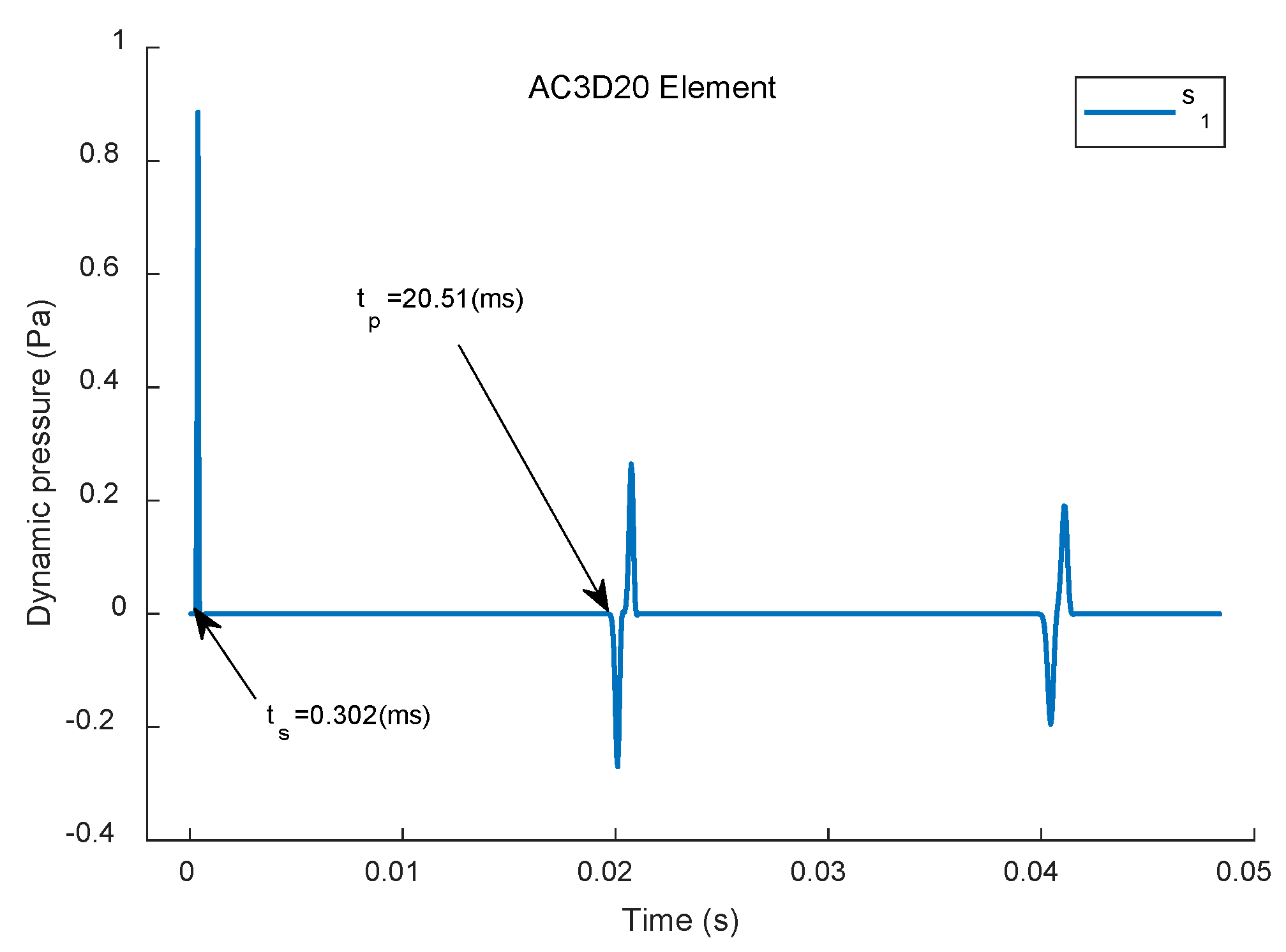
A magnified plot of the dynamic pressure versus time waveform predicted for sensor $s_1$ is shown in Figure 7. Considering the predicted times of flight, the wave speed can be deduced from the arrival times predicted for sensor locations $s_1$ to $s_6$ using the following relation:

$$c=\frac{\Delta \ell }{\Delta \mathrm{t}}=\frac{2\times \left(\ell -l_s\right)}{t_p-t_s}$$

(16)

where $\ell$ is the pipe length $\left(\mathrm{m}\right),l_s$ is the distance from the pipe inlet to sensor location $\left(\mathrm{m}\right)$, c is the wave speed, $t_p$ is the time it takes the wave to travel from the inlet to the sensor then to the pipe exit and back to sensor location $\left(\mathrm{s}\right)$ and $t_s$ is the time it takes the wave to travel from the inlet to sensor location $s_n$ ($\mathrm{s}$).

Substituting the respective data in Equation (16) for sensor $s_1$ gives;

$$c=\frac{2\times \left(4.12-0.128\right)}{\left(20.51-0.302\right)\left(\times {10}^{-3}\right)}\approx 395.09{\mathrm{ms}}^{-1}$$

Similarly, the wave speed c, according to the time of flight for other sensor points ($s_1–s_6$) are computed and tabulated in Table 1. Using the properties of air used for the AFE analysis, the actual speed of sound in air is approximately $345{\mathrm{ms}}^{-1}$. Comparison of the derived sound speed (derived from the predicted arrival times) with the actual sound speed used in the AFEA gives the errors $\mathrm{E}$ associated with each sensor location, as shown in the fifth column of Table 1. These errors are rather large and unacceptable. They can be attributed to the coarseness of the mesh used in the Abaqus AFEA. Therefore, there is a need for mesh refinement, in order to get a more accurate result. This refinement is a bit challenging; as the model size will become bigger, the computation time will be too long and the grid cells will be too much to be numerically computed on a regular computer.

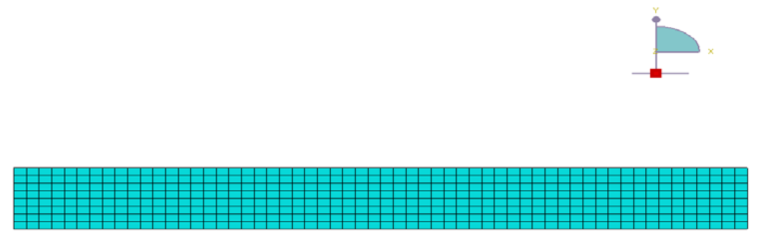
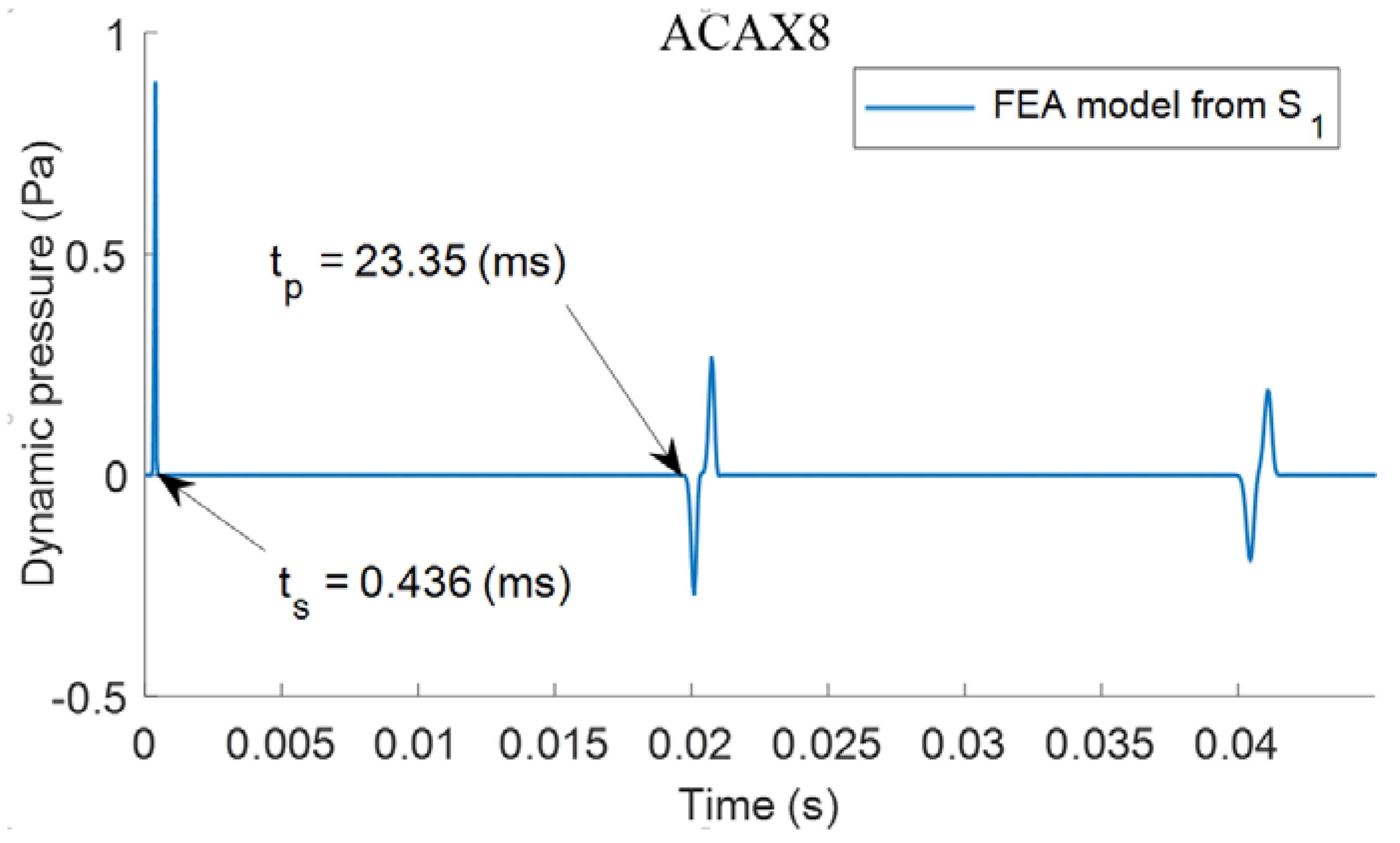
In order to use a finer mesh size without increasing the model size, axisymmetric element types were also used in the simulation. AFEA of acoustic wave propagation in an intact air-filled pipe was conducted using solid axisymmetric element type ACAX8, as illustrated in Figure 8. With this axisymmetric element type, it was possible to use very refined element sizes of 1 mm, and even down to 0.01 mm, for the simulations on a desktop PC with standard specifications, whereas the use of the solid element types AC3D8 and AC3D20 was not possible for element mesh size less than 9 mm. The predicted wave propagation using element type ACAX8 for the smallest mesh size is shown in Figure 9. Similarly, the Time of Flight approach was used to verify the acoustic speed results from the arrival time predicted for sensor locations $s_1$ extracted from Figure 10.

Similarly, by using the properties of air used for the FEA analysis, the actual speed of sound in air is approximately $345{\mathrm{ms}}^{-1}$. Comparison of the derived sound speed (derived from the predicted arrival times) with the actual sound speed used in the AFEA gives the errors ($\mathrm{E}$) associated with each sensor location, as shown in the sixth column of Table 1. These errors are very small in comparison to the errors associated with the use of the AC3D20 element. The relatively very small errors associated with the use of the ACAX8 element type indicate that the axisymmetric elements are better suited for acoustic wave propagation simulations than the AC3D20 element type. Nevertheless, it is seen from

Table 2. Arrival Time of Compression and Rarefaction Wave-front using the acoustic continuum axisymmetric 8-node element (ACAX8).

${\mathit{s}}_{\mathit{n}}$	${\mathit{l}}_{\mathit{s}}\mathbf{\left(}\mathbf{m}\mathbf{\right)}$	${\mathit{t}}_{\mathit{s}}\mathbf{\left(}\mathbf{ms}\mathbf{\right)}$	${\mathit{t}}_{\mathit{p}}\mathbf{\left(}\mathbf{ms}\mathbf{\right)}$	$\mathit{c}$$\mathbf{\left(}{\mathbf{ms}}^{\mathbf{-}\mathbf{1}}\mathbf{\right)}$	Error, $\mathbf{E}\mathbf{(}\mathbf{\%}\mathbf{)}$
$s_1$	0.128	0.43	23.3	$348.4$	0.9
$s_2$	0.938	2.76	21.0	$348.5$	1.0
$s_3$	1.758	5.08	18.7	$346.9$	0.5
$s_4$	2.240	6.49	17.2	$348.2$	0.9
$s_5$	3.050	8.81	14.9	$347.7$	0.7
$s_6$	3.870	11.1	12.6	$357.1$	3.5

that the errors associated with sensor location $s_6$ is about 3.5 to 7 times that of the errors associated with the other sensor locations. This is due to the closeness of sensor $s_6$ to the end of the open-ended pipe outlet where the acoustic wave is reflected.

$$c=\frac{2\times \left(4.12-0.128\right)}{\left(23.35-0.436\right)\left(\times {10}^{-3}\right)}\approx 348.43{\mathrm{ms}}^{-1}$$

4.3.2. Sensitivity of Acoustic Finite Elements

In this section, a sensitivity analysis is developed for the meshing of the acoustic medium. The aim is to investigate the influence of mesh element type and mesh size in acoustic FEA. The AC3D20 element in the Abaqus FEA software produced a lot of computational errors in the derived acoustic speed, as seen in the sixth column of Table 1. Most of the errors in the acoustic speed are more than 15%. To address this much more closely, the two axisymmetric element types ACAX4 and ACAX8 and the two solid element types AC3D8 and AC3D20 were used. Also, various mesh densities were employed involving element seed sizes of 120 mm down to 0.01 mm. While it was possible to run these analyses using the axisymmetric element types ACAX4 and ACAX8 on a regular desktop PC (which has a single processor), the analyses using the solid element types AC3D8 and AC3D20 could only be carried out on supercomputers using multiple cores (between 4 and 12 parallel processors). The results of these sensitivity analyses are shown in Figure 11, Figure 12 and Figure 13.

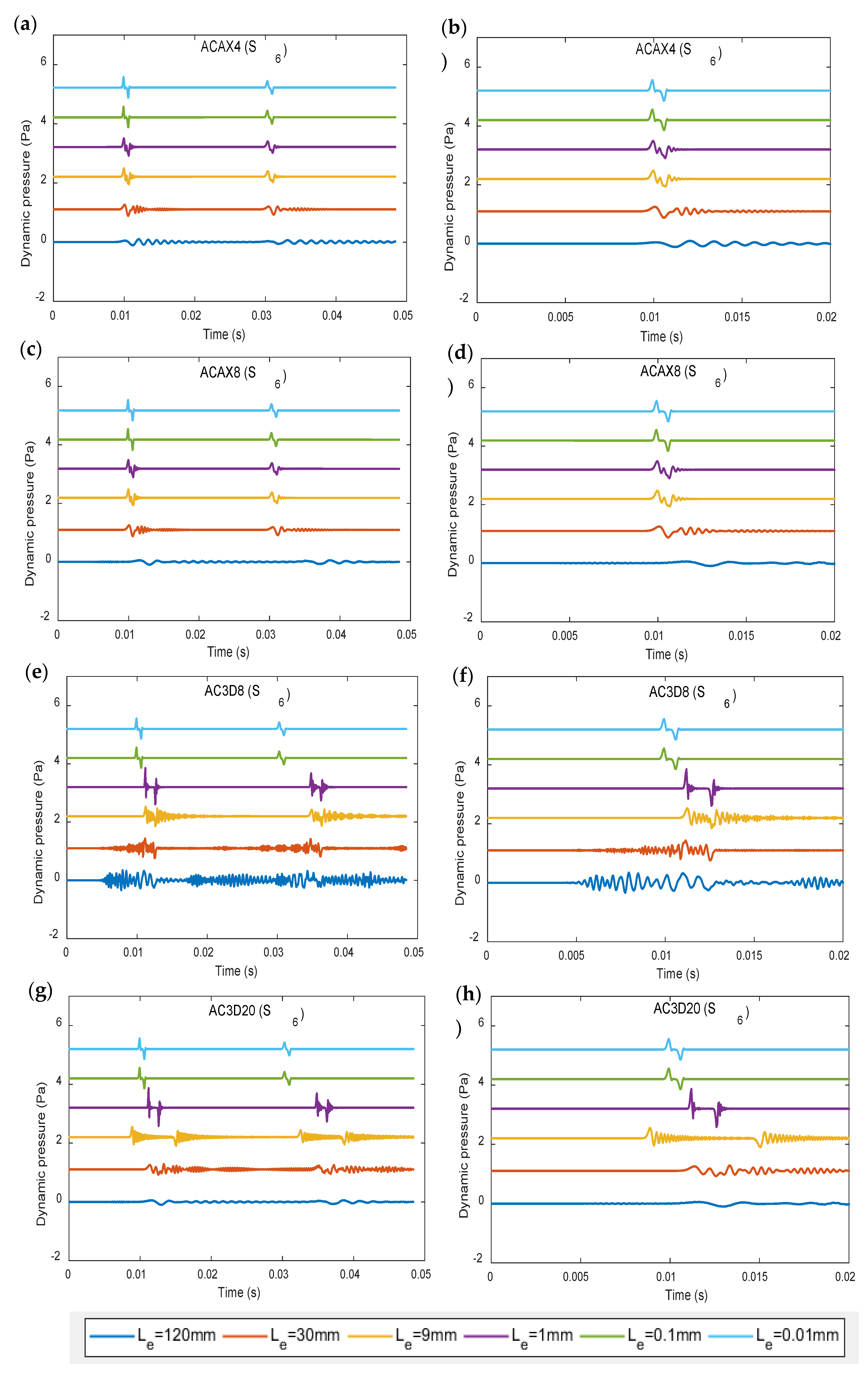
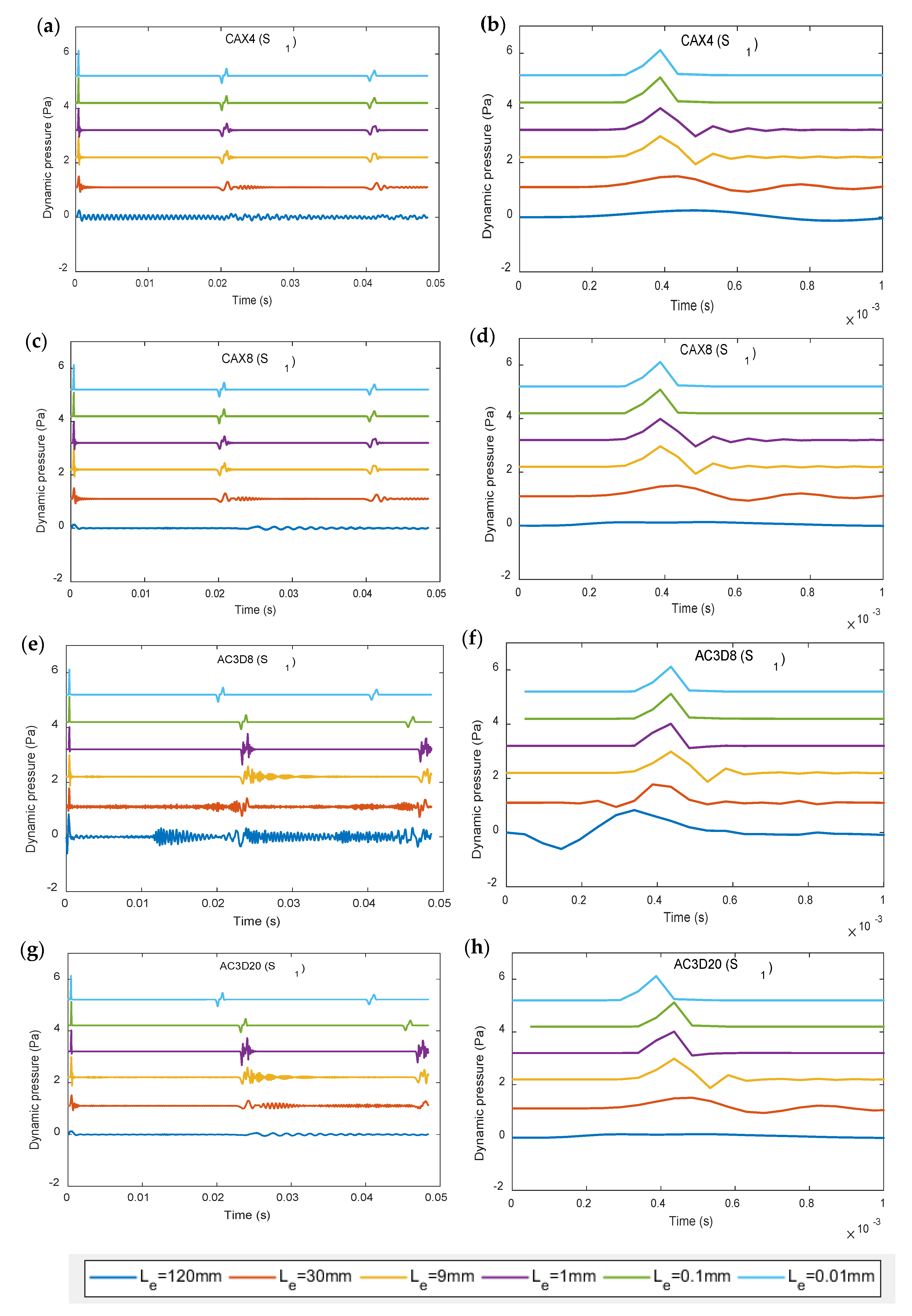
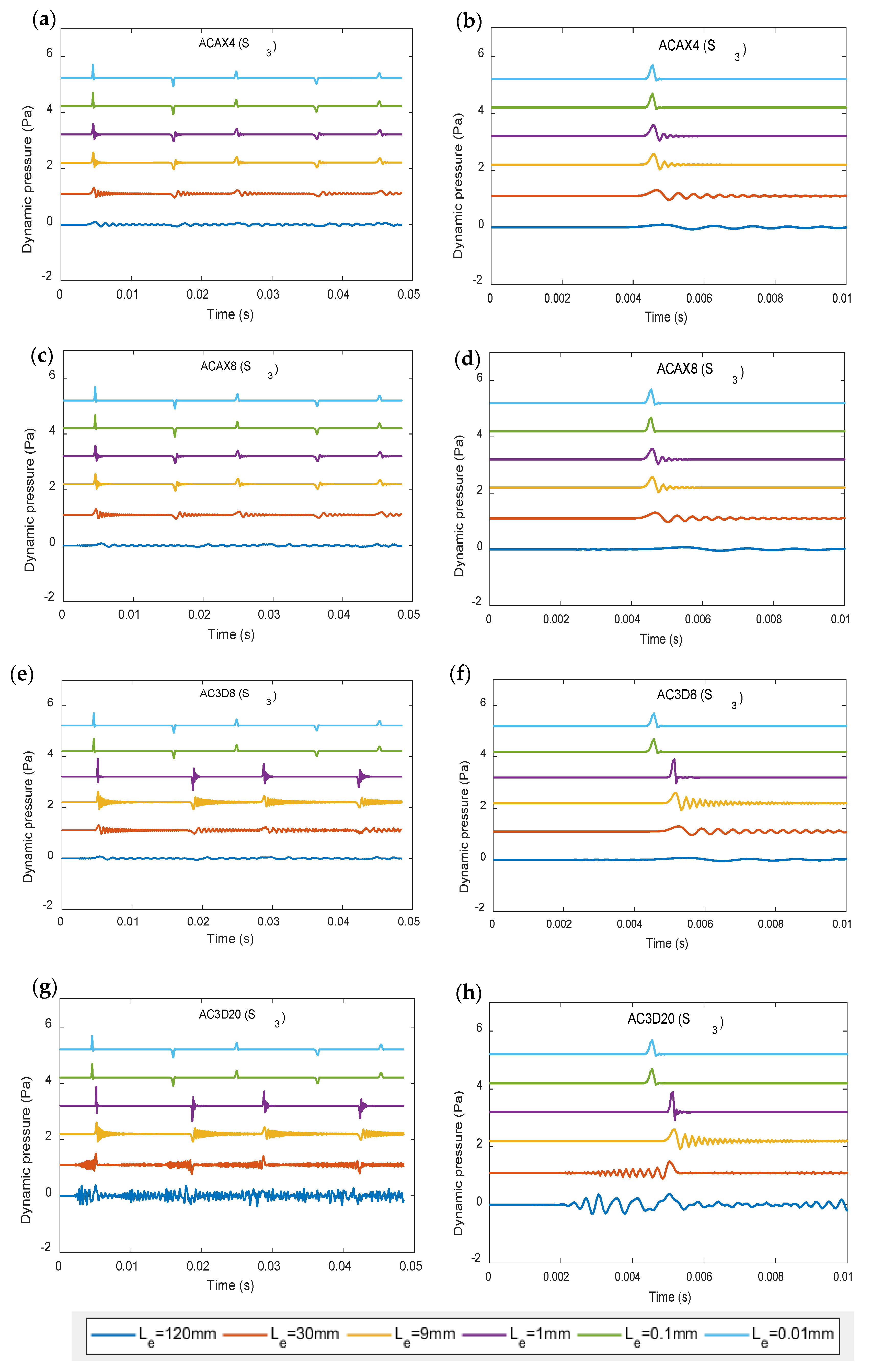
Figure 11, Figure 12 and Figure 13 show the pressure vs. time histories predicted using the two axisymmetric element types, ACAX4 and ACAX8, and the two solid element types, AC3D8 and AC3D20, predicted at sensor locations $s_1,s_3$ and $s_6$ respectively. These pressure-time histories manifest the relationships between the element types chosen for the analyses, the mesh densities used, and the computational errors. The first waveforms for each set of pressure-time histories were also magnified in order to clearly show the differences in the predictions using different element types and mesh densities.

Firstly, the axisymmetric element type ACAX4 was used with a very coarse mesh density of element length L_e = 120 mm to discretise the model. It can be seen from Figure 11a, Figure 12a and Figure 13a, and the corresponding enlarged plots of Figure 11b, Figure 12b and Figure 13b, that the predicted waveforms are not well-separated pulses, but are rather wavy and very noisy curves. The model was refined using L_e = 30 mm; this resulted in a less noisy waveforms, but not well-defined pulses. By further refinement using L_e = 9 mm, the waveforms become a little clearer, with well-defined pulses and only a little noise. Very refined mesh density of L_e = 0.1 mm and L_e = 0.01 mm was further used, and the waveforms become very smooth, clear, identical, and well-defined. Thus, it can be deduced that the AFEA solution becomes more accurate when element type ACAX4 with length L_e = 0.1 mm is used for the analyses.

These analyses were repeated using the axisymmetric element ACAX8 with the same mesh densities as those previously used with the element type ACAX4. The predicted waveforms are shown in Figure 11c, Figure 12c, and Figure 13c, and the corresponding enlarged plots of the first pulses are shown in Figure 11d, Figure 12d, and Figure 13d, respectively. These figures show that the characteristics predicted by the ACAX8 element type are similar to those predicted by the ACAX4 element type. That is, the predicted waveforms are not well-separated pulses, but are rather wavy and very noisy curves when coarse mesh densities are used. However, when fine mesh densities are used, the waveforms become very smooth, clear, and well-defined. Furthermore, the converged waveforms predicted by the ACAX8 element type are identical to those predicted by the ACAX4 element type. The main difference between the two element types is that the ACAX8 element type required greater computational times.

In the introduction, it was stated that Owowo and Oyadiji [11] used 3D hexahedral acoustic elements which they expected to give accurate predictions, just as the 3D hexahedral structural elements give accurate predictions for structural problems. But it was shown in the previous sub-section and in Table 1 that the hexahedral acoustic element type AC3D20 gives large prediction errors even when the element size used is deemed to be reasonably small. In order to ascertain the mesh sensitivity versus accuracy of the hexahedral acoustic element types AC3D8 and AC3D20, they were also used in the acoustic simulations for the same mesh densities as those used with the axisymmetric element types ACAX4 and ACAX8.

Figure 11e–h, Figure 12e–h, and Figure 13e–h show that when coarse mesh densities (i.e., L_e = 120 mm, L_e = 30 mm and L_e = 9 mm) are used with element types AC3D8 and AC3D20, the predicted waveforms are worse than those predicted by the axisymmetric elements. The predicted waveforms are not well-separated pulses, but are rather very wavy and very noisy curves. When a fine mesh is used (L_e = 1 mm), the waveforms become less noisy and show well-defined pulses.

Figure 11 also shows that when the mesh is coarse, the waveforms predicted by the solid element type AC3D20 are less noisy than the waveforms predicted by the solid element types AC3D8. When the mesh is very fine (i.e., L_e = 0.1 mm and L_e = 0.01 mm), the predictions of the two element types are identical. However, the analysis using element type AC3D20 takes much more time to complete than with element type AC3D8. Furthermore, the use of AC3D20 elements generates a much bigger model and requires more static and dynamic storage than the use of AC3D8 elements.

In addition to the predicted waveforms not being sufficiently smooth with well-defined pulses when a fine mesh is used (L_e = 1 mm), the figures also show that the predicted time intervals between the pulses is also larger, resulting in large errors in the predicted acoustic wave velocity. Thus, while it is important for the waveforms to be as smooth as possible, it is not sufficient to judge the accuracy of an acoustic wave propagation analysis by the waveform alone; it is also necessary to consider the accuracy of the Time of Flight.

The performance of the FEA solutions for different element types and mesh sizes is evaluated using three key variables, namely: (1) the waviness of the waveforms; (2) the computational time of the analysis; and (3) the predicted acoustic speed error. The variations of these variables are examined using different acoustic element types and sizes in the Abaqus FEA software. The relevant sensitive parameters employed by the analysis for each element type and element sizes are summarised in

Table 3. Basic acoustic mesh sensitivity study.

Element Type	$\mathbf{Mesh}\mathbf{Seed}{\mathbf{L}}_{\mathbf{e}}\mathbf{\left(}\mathbf{mm}\mathbf{\right)}$	Total No. of Element	Total No. of Nodes	Total No. of Variables	Analysis Time (h)
ACAX4 (1)	120	35	72	72	3
	30	136	274	274	4.5
	9	1374	1836	1836	6
	1	103,000	107,146	107,146	7
	0.1	2,475,400	2,612,980	2,612,980	8.5
	0.01	13,305,460	13,937,450	13,937,450	10
ACAX8	120	35	178	178	3.5
	30	136	683	683	5
	9	1374	3836	3836	8
	1	103,000	317,291	317,291	9.5
	0.1	2,475,400	3,085,430	3,085,430	11
	0.01	13,305,460	15,135,560	15,135,560	12
AC3D8 (2)	120	432	629	629	24
	30	1584	2261	2261	36
	9	5328	7565	7565	46
	1	128,000	164,041	164,041	60
	0.1	22,776,000	23,235,670	23,235,670	132
	0.01	63,085,430	64,587,604	64,587,604	220
AC3D20	120	432	2277	2277	30
	30	1584	8229	8229	46
	9	5328	27,573	27,573	57
	1	128,000	616,113	616,113	71
	0.1	22,776,000	28,458,752	28,458,752	179
	0.01	63,085,430	113,654,300	113,654,300	240

⁽¹⁾ acoustic continuum axisymmetric 4-node element; ⁽²⁾ acoustic continuum 8-node brick element

.

4.3.3. Comparisons of Prediction Errors Due to Acoustic Element Type

Table 4. Acoustic mesh sensitivity study showing the acoustic speed computation error.

Element Type	$\mathbf{Acoustic}\mathbf{Wave}\mathbf{Speed}\mathbf{\left(}{\mathbf{ms}}^{\mathbf{-}\mathbf{1}}\mathbf{\right)}$						Error (%)
	${\mathbf{L}}_{\mathbf{e}}\mathbf{\left(}\mathbf{mm}\mathbf{\right)}$						${\mathbf{L}}_{\mathbf{e}}\mathbf{\left(}\mathbf{mm}\mathbf{\right)}$
	120	30	9	1	0.1	0.01	120	30	9	1	0.1	0.01
ACAX4	354.1	353.7	353.2	352.4	349.3	348.4	2.6	2.5	2.4	2.1	1.2	0.9
ACAX8	352.6	352.4	352.4	351.6	349.0	348.4	2.2	2.1	2.1	1.9	1.1	0.9
AC3D8	396.3	395.4	395.3	395.4	381.0	$350.5$	14.9	14.6	14.5	14.6	10.4	1.5
AC3D20	395.9	395.1	395.0	395.0	380.4	349.9	14.8	14.5	14.4	14.4	10.2	1.4

shows the acoustic wave speed derived from the waveforms predicted by the four acoustic element types using different mesh densities based on the Time of Flight approach. The percentage errors associated with these predicted velocities are also shown in the table. A summary of the requirements, performance, and associated errors for the four acoustic element types in the predictions of the acoustic wave propagation is shown in

Table 5. Sensitivity analysis- key variable performance evaluation.

Element Type	Refinement	Quality	NE	NN	TC (h)	C (ms−1)	$\mathbf{E}\mathbf{(}\mathbf{\%}\mathbf{)}$
AC3D20	Coarse	Noisy	1584	8229	46	$395.1$	14.5
AC3D8	Coarse	Noisy	1584	2261	36	$395.4$	14.6
AC3D20	Fine	Smooth	6.31 × 107 (1)	1.13 × 108 (3)	240	$349.9$	1.4
AC3D8	Fine	Smooth	6.31 × 107 (1)	6.45 × 107 (4)	220	$350.5$	1.5
ACAX8	Coarse	Noisy	136	683	5	$352.4$	2.1
ACAX4	Coarse	Noisy	136	274	4.5	$353.7$	2.5
ACAX8	Fine	Smooth	1.33 × 107 (2)	1.51 × 107 (5)	12	348.4	0.9
ACAX4	Fine	Smooth	1.33 × 107 (2)	1.39 × 107 (6)	10	348.4	0.9

NE = number of elements generated; NN = number of nodes generated; E = Error; C = Speed; TC = computational time, exact values: ⁽¹⁾ 63,085,430; ⁽²⁾ 13,305,460; ⁽³⁾ 113,654,300; ⁽⁴⁾ 64,587,604; ⁽⁵⁾ 15,135,560; ⁽⁶⁾ 13,937,450.

.

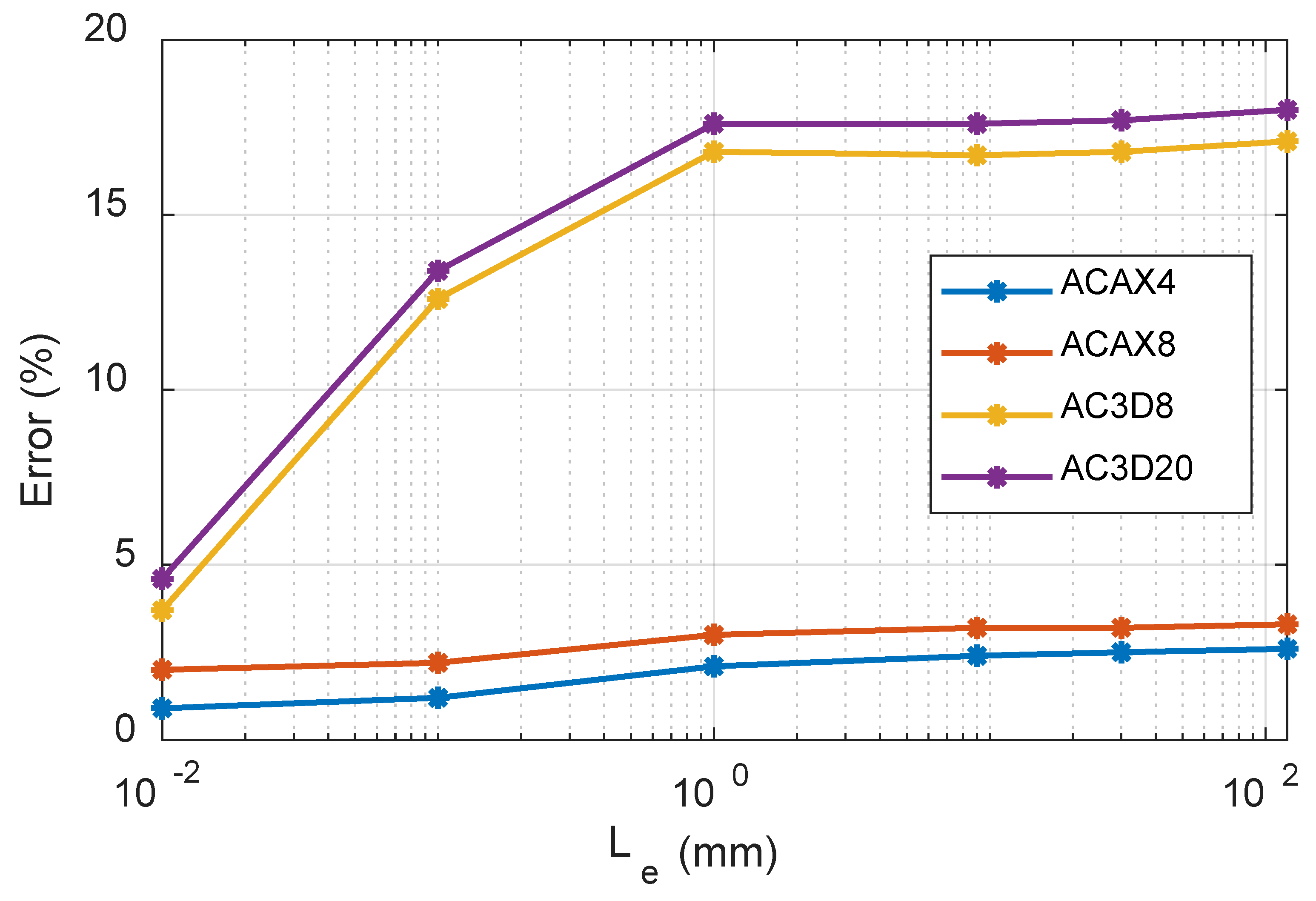
Figure 14 shows the variations of the percentage acoustic speed errors with the element sizes for the four acoustic element types. It is observed that the axisymmetric element type ACAX4 and ACAX8 produce less computational errors in the acoustic FEA. Also, it is clearly seen that the linear interpolation elements (ACAX4 and AC3D8) have less errors than the quadratic interpolation elements (ACAX8 and AC3D20). Figure 14 shows that very large computational errors occur in the AFE analysis result when solid element types AC3D8 and AC3D20 are used. But when the axisymmetric element types ACAX4 and ACAX8 are used, the errors are minimised.

It is thus concluded that the solid element types AC3D8 and AC3D20 are not optimal in terms of speed, accuracy, and computation-resource requirements for AFE analysis of acoustic wave propagation in an air-filled pipe. Furthermore, considering the computational time and resources for each model as illustrated in Table 5, the ACAX4 is the best element type for acoustic FEA. This is because it has the smallest model size, smallest computational time, and smallest computational errors.

5. Conclusions

The acoustic finite element approach has been used to predict the wave propagation characteristics in a fluid-filled pipe. This paper has detailed the use of Finite Element Analysis (FEA) to simulate the acoustic wave propagation and acoustic wave reflectometry of a pipe. The wave velocity predicted by the FEA has been found to be consistent with the actual velocity when the right element type is chosen for the numerical computation. The primary conclusions of this paper are as follows.

• The acoustic FEA of a fluid-filled pipe can be achieved with the simulation of only the fluid content of the pipe and without the inclusion of the pipe in the model. Thus, this eliminates contact interaction of the solid pipe wall and the fluid, and as a consequence, reduces computational time and resources. Since the specific acoustic impedance of the air medium is much smaller than the specific impedance of the wall of a metallic or plastic pipe, this assumption is reasonable. The results confirm that the acoustic FEA of an air-filled pipe can be achieved with the simulation of only the fluid content of the pipe and without the inclusion of the pipe in the model. However, when a denser fluid medium is used, and when there is high flow velocity, fluid-structure interaction will become very significant. Then, the fluid medium and the pipe wall will need to be modelled together.
• The main source of error in an acoustic FEA is the element type chosen and the mesh density. The results indicate that the ACAX4 element type with a fine mesh should be used in any acoustic FEA simulation of wave propagation in a symmetrical pipe in order to obtain the smallest computational errors, fastest computations, and least usage of computer static and dynamic storage resources. For a nonsymmetrical pipe, the 3D solid hexahedral elements can be used at the part of the pipe that is unsymmetrical and the 2D-like axisymmetric element should be used at the symmetric part of the pipe to obtain the smallest computational errors, fastest computations, and least usage of computer static and dynamic storage resources.
• It has been shown that the use of the Time of Flight approach enables the verification of the accuracy of the acoustic FEA simulations using any of the four element types investigated, namely: ACAX4, ACAX8, AC3D8, and AC3D20.
• Of these four element types, the best element for AFE simulations of wave propagation in a symmetric air-filled pipe was found to be the axisymmetric element type ACAX4, whereas the worst element type was found to be the solid element type AC3D20. This is a rather surprising result when compared to the equivalent structural analysis, in which the solid elements with quadratic interpolation are better than element types with linear interpolation for the same mesh density.