Towards Enhanced Performance of Neural-Network-Based Fault Detection Using an Sequential D-Optimum Experimental Design


Abstract
:1. Introduction
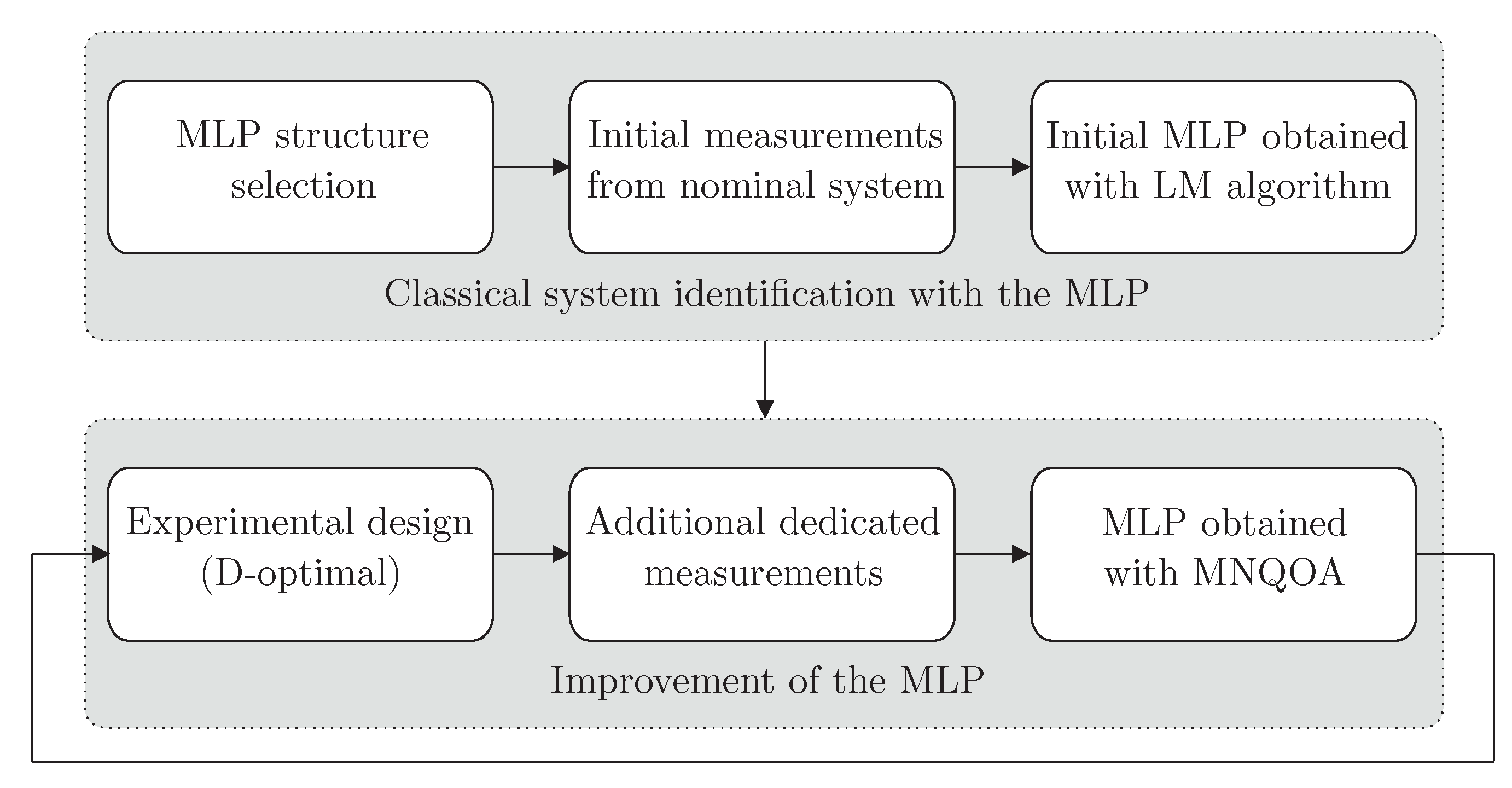
- It is based on the classical approach to training neural networks and can be realized with state-of-the-art approaches available in the literature;
- Having, an initial structure and parameters of a neural network a novel Modified Nonlinear Quasi-OBE Algorithm (MNQOA) with optimal input sequence is used to gradually decrease its uncertainty. After this process, an adaptive threshold is obtained for the resulting neural network.
- The neural network obtained in Stage 2 along with an associated adaptive threshold are used for the on-line RFD.
2. Related Works: Active and Passive Approaches to Fault Detection
- fault detection:
- it makes it possible to undertake a diagnostic decision concerning the fault. In other words, it provides a binary decision concerning the fault, e.g., a pump is faulty;
- fault isolation:
- it enables to determine the location of the fault, e.g., an induction motor driving the pump is faulty;
- fault estimation:
- it allows to determine the size of the fault as well as its time varying nature, e.g., the induction motor driving the pump is faulty and it losts 20% of its performance.
- Active fault detection:
- aims at eliminating modeling uncertainty;
- Passive fault detection:
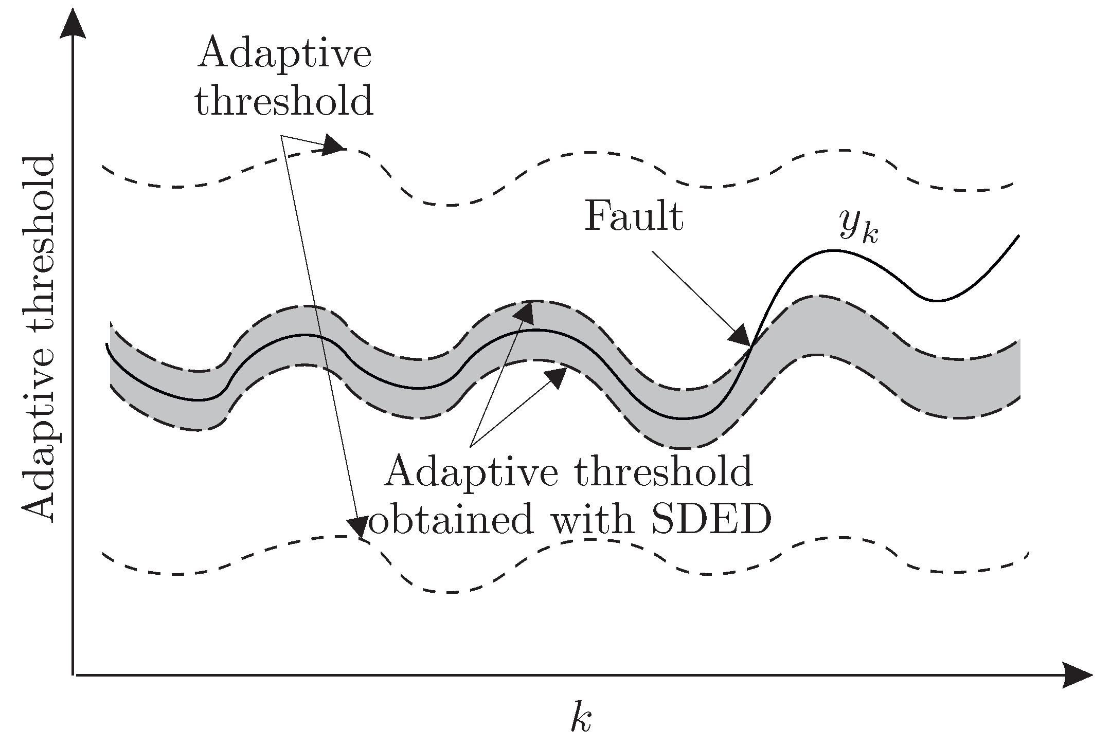
- focuses on providing a adaptive threshold forming an enclosure associated with modeling uncertainty.
3. Model-Based RFD
4. Modified Non-Linear Quasi OBE Algorithm
- Initialization:
- where is a large constant and is initial parameter estimate.
- Sequential iteration:
- Calculate:if thenelse:
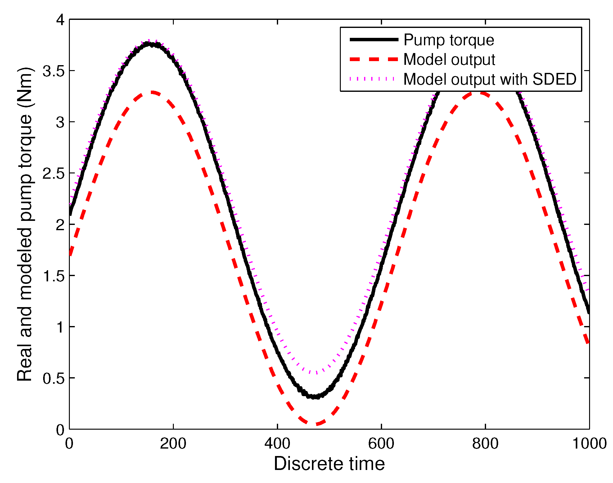
5. Enhancing Performance of Neural Networks with SDED
- Step 1:
- Set , determine an initial parameter by exploiting the collected input-output data measurement set of the diagnosed system in the nominal state, set where denotes sufficiently large constant. Select , the number of gradual improvement iterations.
- Step 2:
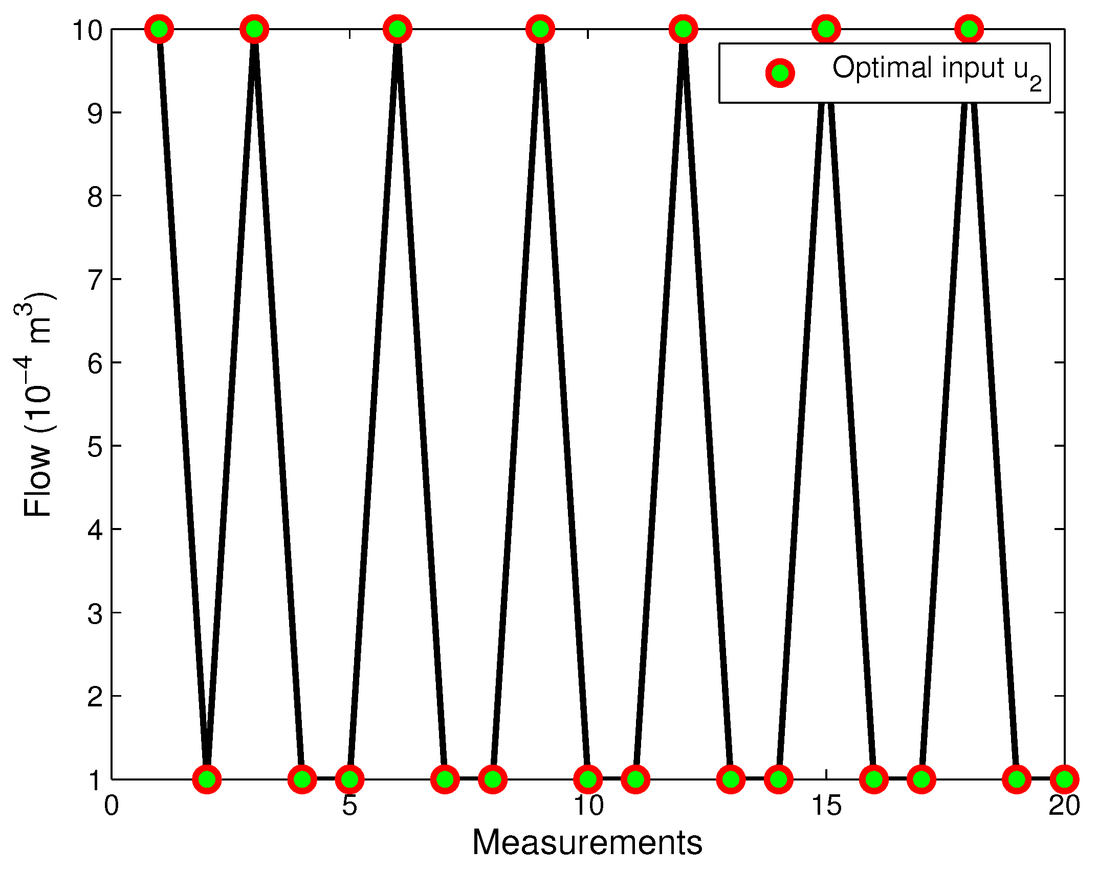
- Obtain by D-optimal input value, and then fed it into the modeled system to get .
- Step 3:
- Update the parameter estimate. If then STOP the algorithm, else set and go to Step 2.
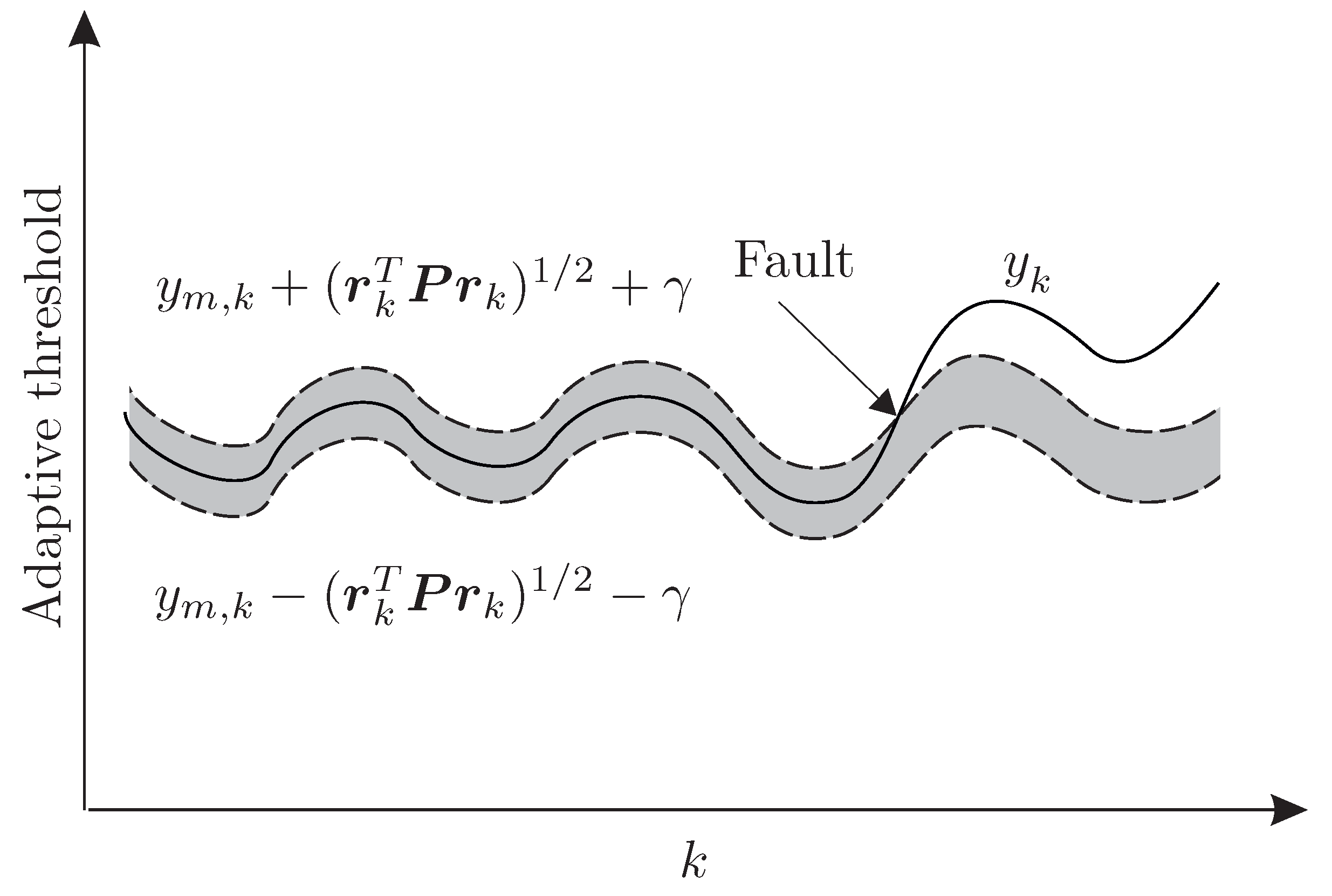
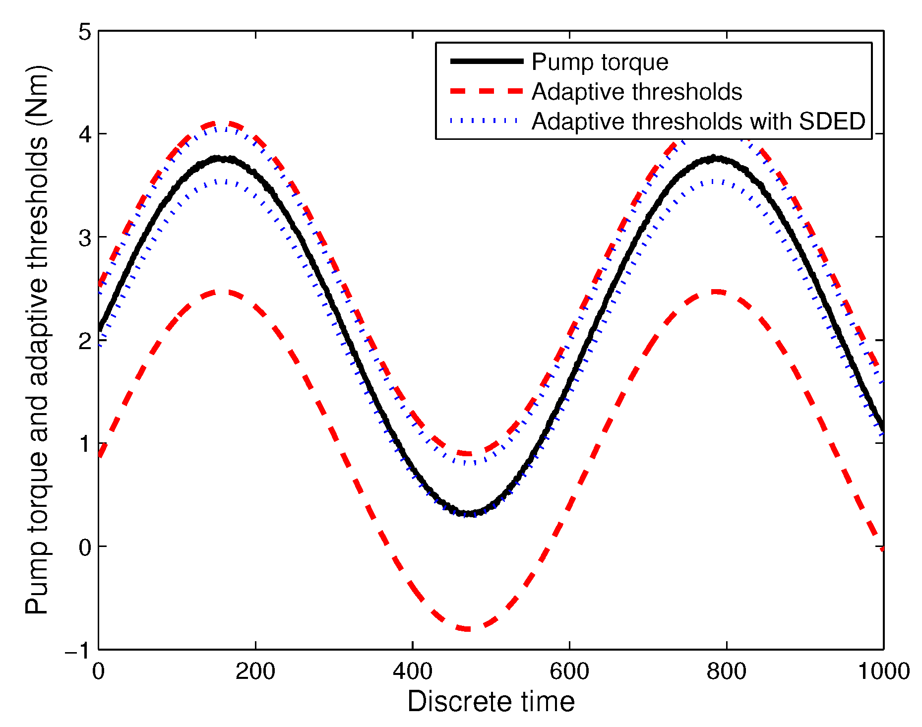
6. Adaptive Thresholds for the RFD
7. An Illustrative Example of the RFD
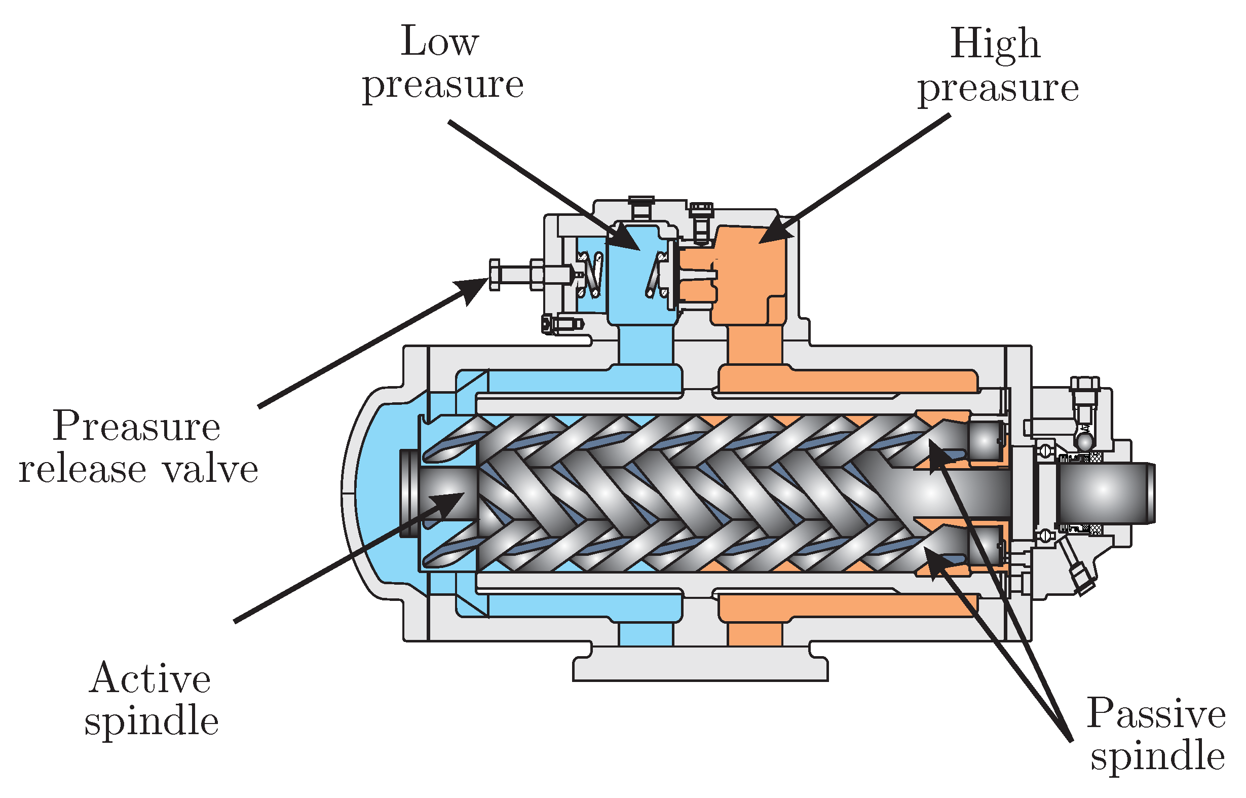
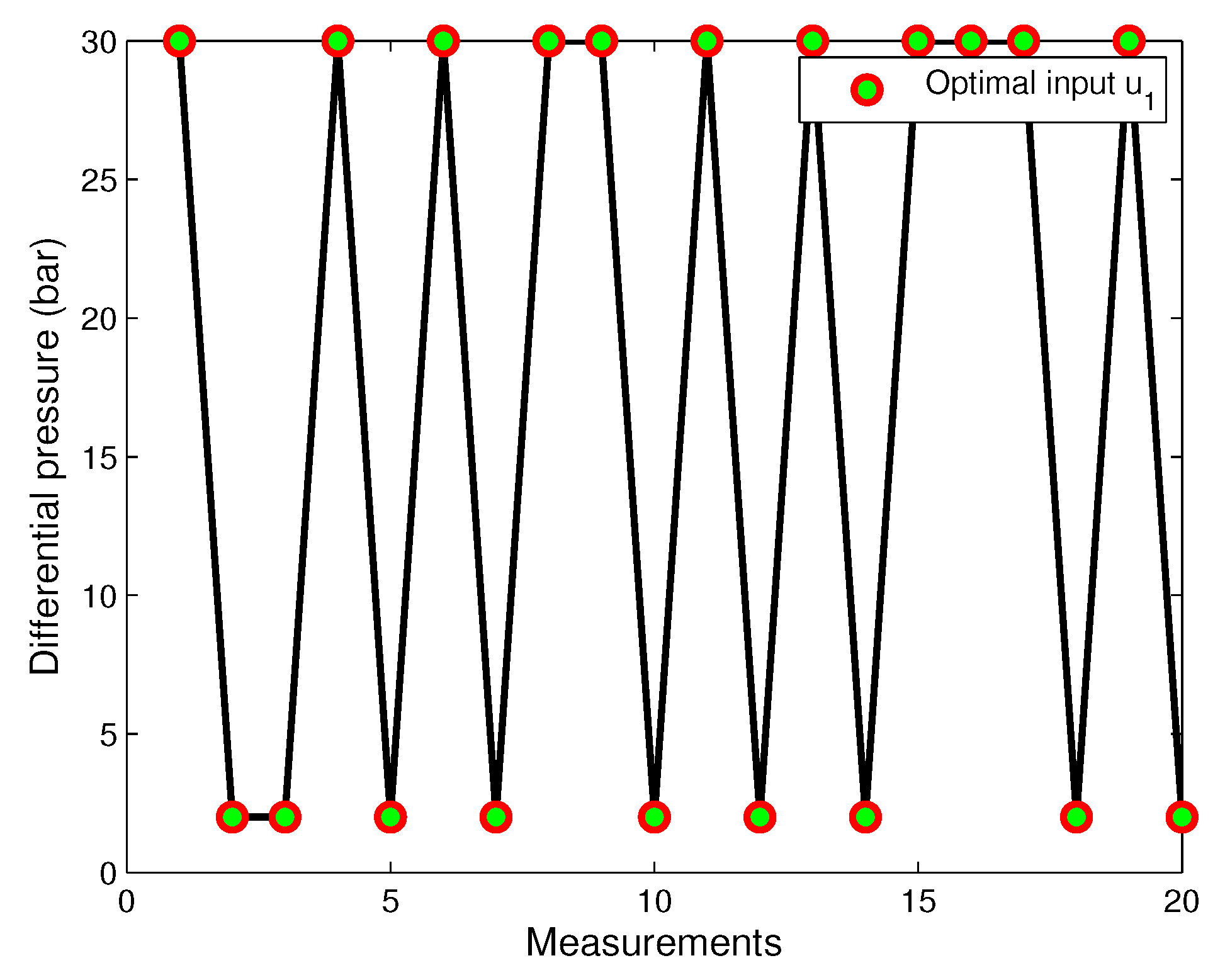
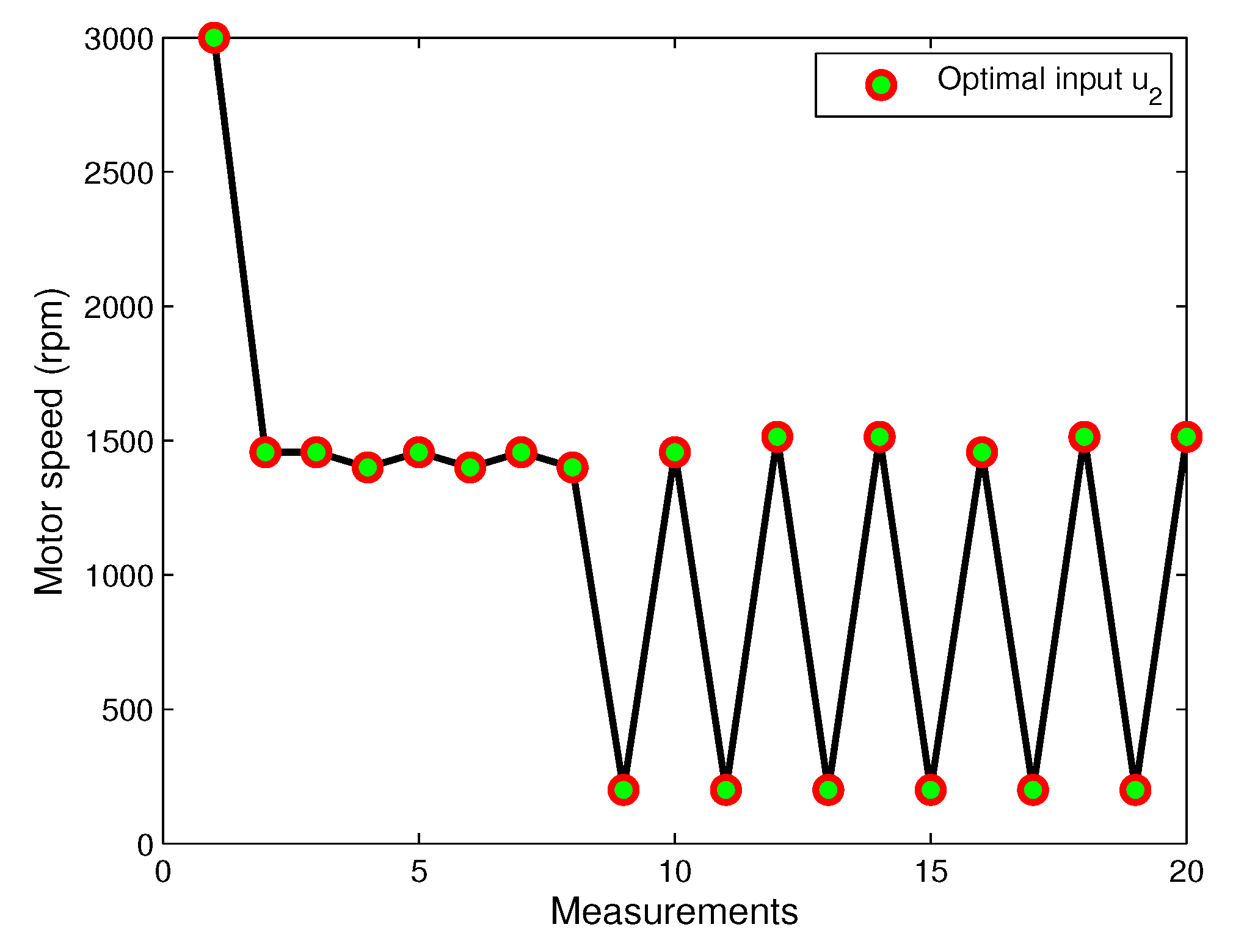
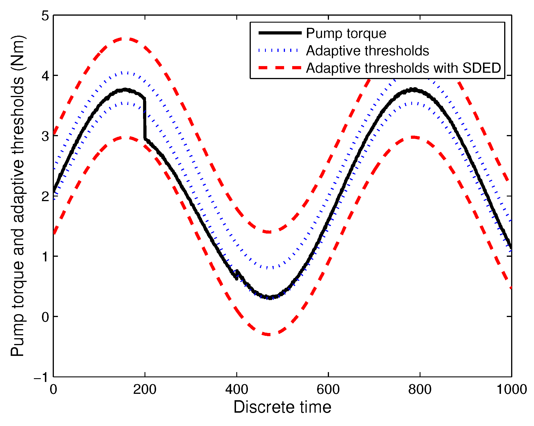
7.1. Experimental Study with the Three-Screw Spindle Oil Pump
- —the differential pressure between inlet and outlet of the pump,
- —the motor speed,
- —the torque of the pump.
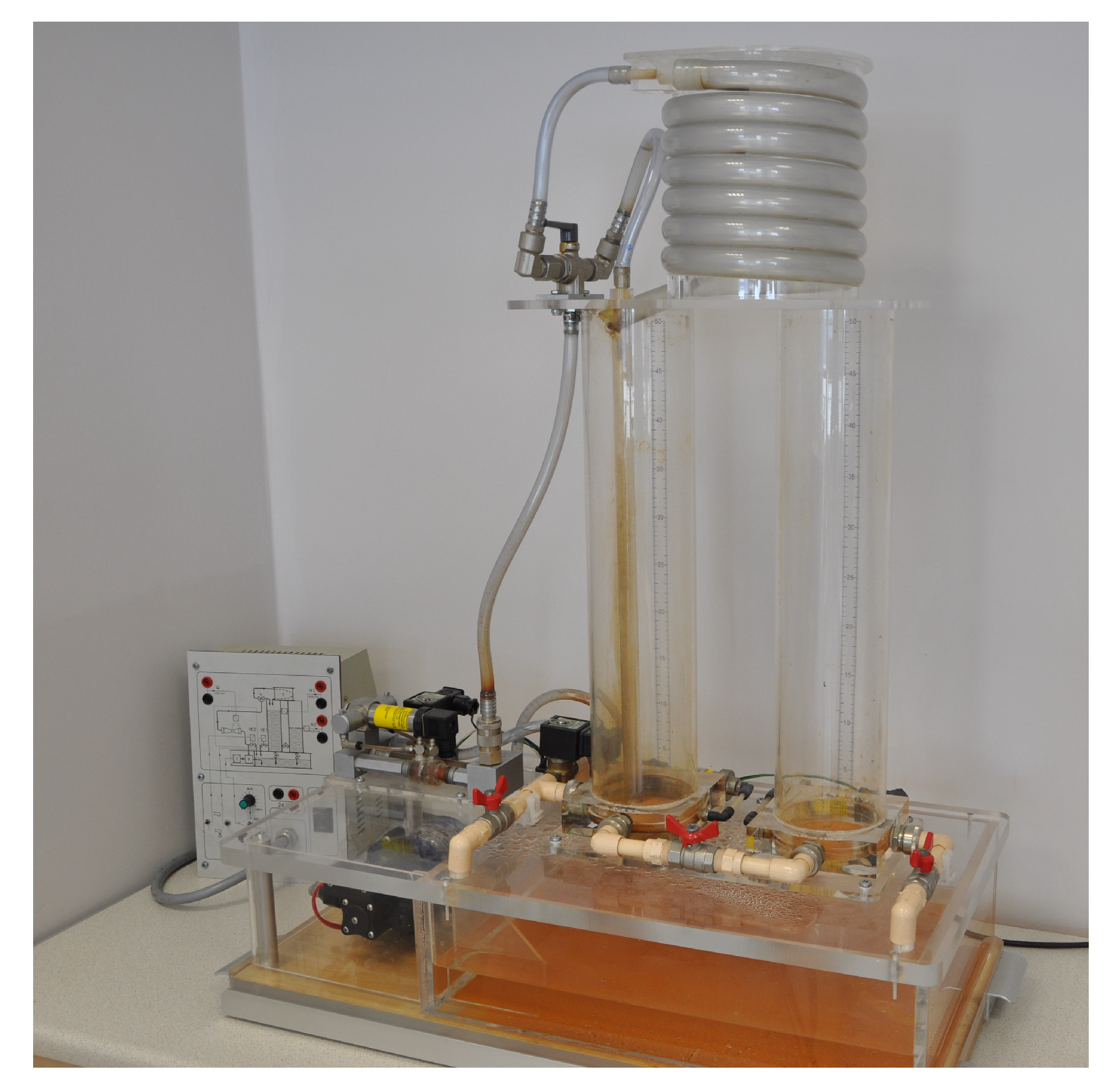
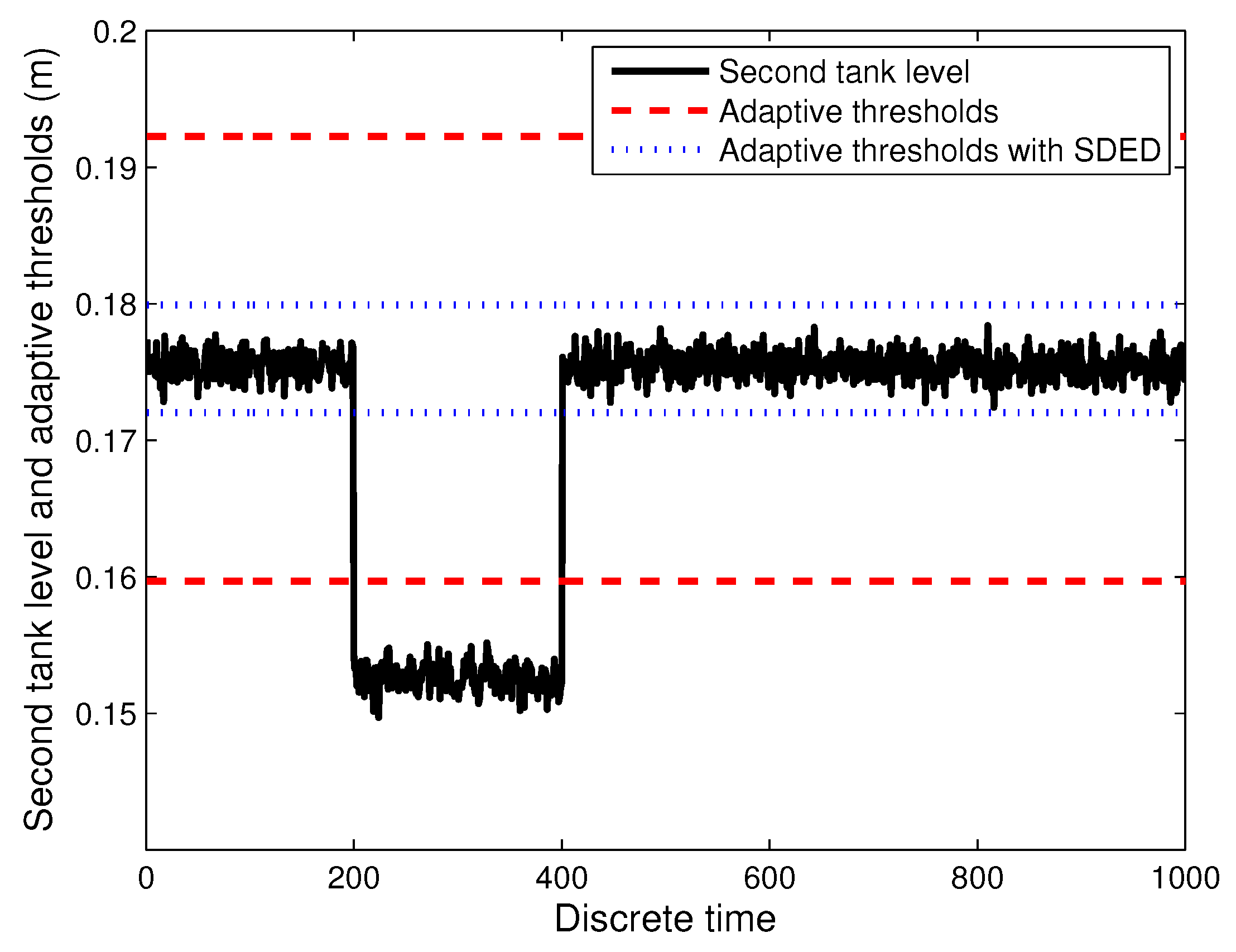
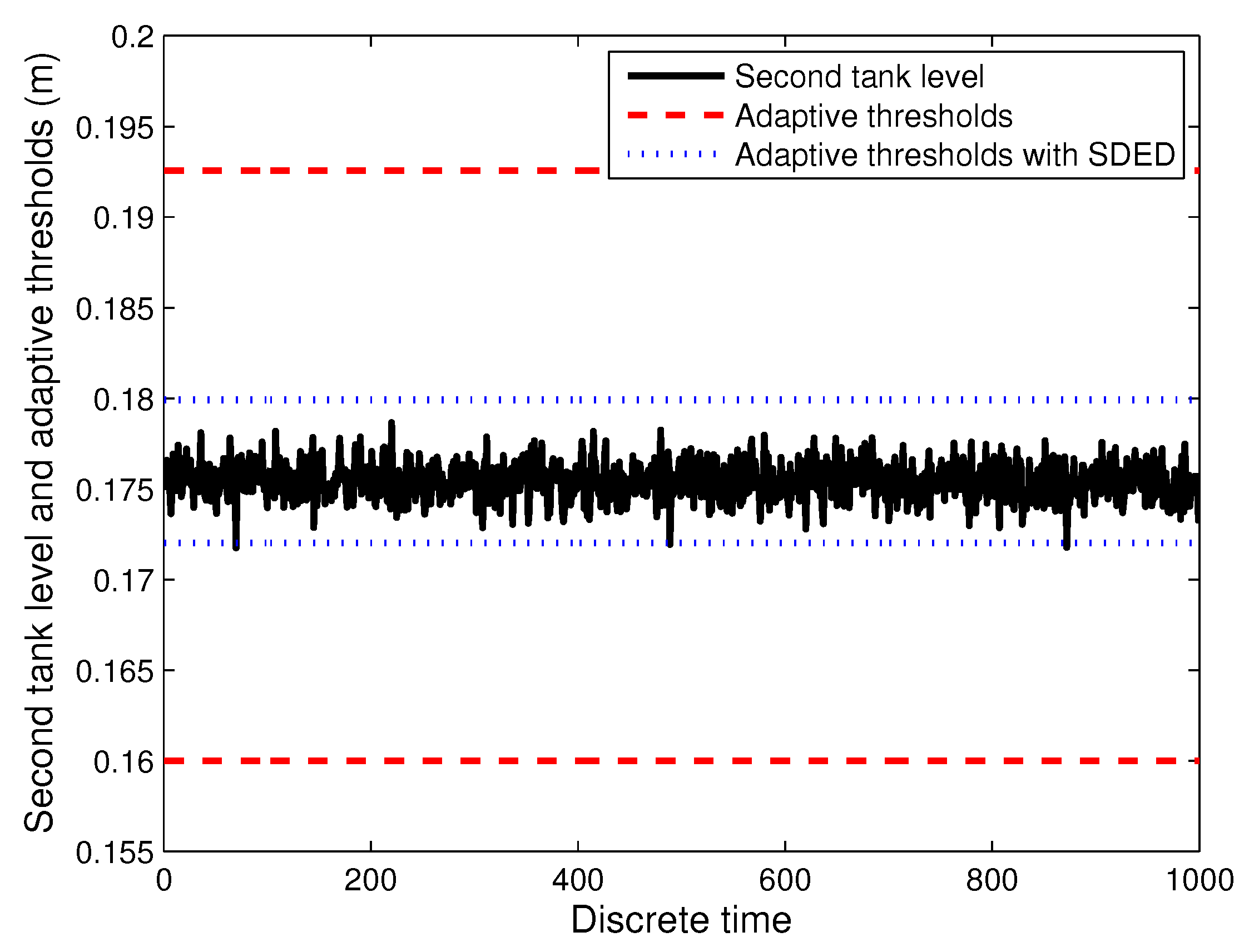
7.2. Experimental Study with the Two-Tank System
8. Conclusions
Funding
Conflicts of Interest
References
- Schalkoff, R. Artificial Neural Networks; McGraw-Hill Companies: New York, NY, USA, 2011. [Google Scholar]
- Haykin, S. Neural Networks and Learning Machines; Prentice Hall: New York, NY, USA, 2009. [Google Scholar]
- Nelles, O. Non-Linear Systems Identification. From Classical Approaches to Neural Networks and Fuzzy Models; Springer: Berlin/Heidelberg, Germany, 2001. [Google Scholar]
- Gao, Z.; Cecati, C.; Ding, S.X. A Survey of Fault Diagnosis and Fault-Tolerant Techniques—Part I: Fault Diagnosis With Model-Based and Signal-Based Approaches. IEEE Trans. Ind. Electron. 2015, 62, 3757–3767. [Google Scholar] [CrossRef] [Green Version]
- Gao, Z.; Cecati, C.; Ding, S.X. A Survey of Fault Diagnosis and Fault-Tolerant Techniques—Part II: Fault Diagnosis With Knowledge-Based and Hybrid/Active Approaches. IEEE Trans. Ind. Electron. 2015, 62, 3768–3774. [Google Scholar] [CrossRef]
- Zolfaghari, S.; Noor, S.; Rezazadeh Mehrjou, M.; Marhaban, M.; Mariun, N. Broken Rotor Bar Fault Detection and Classification Using Wavelet Packet Signature Analysis Based on Fourier Transform and Multi-Layer Perceptron Neural Network. Appl. Sci. 2018, 8, 25. [Google Scholar] [CrossRef]
- Farrar, C.; Worden, K. Structural Health Monitoring: A Machine Learning Perspective; John Wiley & Sons: Hoboken, NJ, USA, 2012. [Google Scholar]
- Blanke, M.; Schröder, J. Diagnosis and Fault-Tolerant Control; Springer: Berlin/Heidelberg, Germany, 2006; Volume 2. [Google Scholar]
- Patton, R.J.; Frank, P.M.; Clark, R.N. Issues of Fault Diagnosis for Dynamic Systems; Springer: Berlin/Heidelberg, Germany, 2000. [Google Scholar]
- Qi, X.; Theilliol, D.; Qi, J.; Zhang, Y.; Han, J.; Song, D.; Wang, L.; Xia, Y. Fault diagnosis and fault tolerant control methods for manned and unmanned helicopters: A literature review. In Proceedings of the 2013 Conference on Control and Fault-Tolerant Systems (SysTol), Nice, France, 9–11 October 2013; pp. 132–139. [Google Scholar]
- Isermann, R. Fault Diagnosis Applications: Model Based Condition Monitoring, Actuators, Drives, Machinery, Plants, Sensors, and Fault-Tolerant Systems; Springer: Berlin/Heidelberg, Germany, 2011. [Google Scholar]
- Cao, M.S.; Ding, Y.J.; Ren, W.X.; Wang, Q.; Ragulskis, M.; Ding, Z.C. Hierarchical Wavelet-Aided Neural Intelligent Identification of Structural Damage in Noisy Conditions. Appl. Sci. 2017, 7, 391. [Google Scholar] [CrossRef]
- Sutton, R.; Barto, A. Reinforcement Learning, An Introduction, 2nd ed.; The MIT Press: Cambridge, MA, USA; London, UK, 2018. [Google Scholar]
- Fogel, E.; Huang, Y.F. On the value of information in system identification? bounded noise case. Automatica 1982, 2, 229–238. [Google Scholar] [CrossRef]
- Milanese, M.; Norton, J.; Piet-Lahanier, H.; Walter, E. Bounding Approaches to System Identification; Plenum Press: New York, NY, USA, 1996. [Google Scholar]
- Cerone, V.; Piga, D.; Regruto, D. Bounded error identification of Hammerstein systems through sparse polynomial optimization. Automatica 2012, 48, 2693–2698. [Google Scholar] [CrossRef] [Green Version]
- Arablouei, R.; Doğançay, K. Modified quasi-OBE Algorithm with Improved Numerical Properties. Signal Process. 2013, 93, 797–803. [Google Scholar] [CrossRef]
- Sanayei, M.; Khaloo, A.; Gul, M.; Catbas, F.N. Automated finite element model updating of a scale bridge model using measured static and modal test data. Eng. Struct. 2015, 102, 66–79. [Google Scholar] [CrossRef]
- Sohn, H.; Farrar, C.R.; Hemez, F.M.; Shunk, D.D.; Stinemates, D.W.; Nadler, B.R.; Czarnecki, J.J. A Review of Structural Health Monitoring Literature: 1996–2001; Los Alamos National Laboratory: Mexico, USA, 2003.
- Dervilis, N.; Worden, K.; Cross, E. On robust regression analysis as a means of exploring environmental and operational conditions for SHM data. J. Sound Vib. 2015, 347, 279–296. [Google Scholar] [CrossRef]
- Xu, H.; Humar, J. Damage detection in a girder bridge by artificial neural network technique. Comput. Aided Civ. Infrastruct. Eng. 2006, 21, 450–464. [Google Scholar] [CrossRef]
- Walter, E.; Pronzato, L. Identification of Parametric Models from Experimental Data; Springer: Berlin/Heidelberg, Germany, 1997. [Google Scholar]
- Atkinson, A.C.; Donev, A.N. Optimum Experimental Designs; Oxford University Press: New York, NY, USA, 1992. [Google Scholar]
- Puig, V.; Quevedo, J.; Tornil, S. Robust Fault Detection: Active Versus Passive Approaches. IFAC Proc. Vol. 2000, 33, 157–163. [Google Scholar] [CrossRef]
- Puig, V.; Stancu, A.; Escobet, T.; Nejjari, F.; Quevedo, J.; Patton, R. Passive robust fault detection using interval observers: Application to the DAMADICS benchmark problem. Control Eng. Pract. 2006, 14, 621–633. [Google Scholar] [CrossRef]
- Ashari, A.E.; Nikoukhah, R.; Campbell, S.L. Active Robust Fault Detection in Closed-Loop Systems: Quadratic Optimization Approach. IEEE Trans. Autom. Control 2012, 57, 2532–2544. [Google Scholar] [CrossRef]
- Padilla, M.; Choinière, D. A combined passive-active sensor fault detection and isolation approach for air handling units. Energy Build. 2015, 99, 214–219. [Google Scholar] [CrossRef]
- Odendaal, H.M.; Jones, T. Actuator fault detection and isolation: An optimised parity space approach. Control Eng. Pract. 2014, 26, 222–232. [Google Scholar] [CrossRef]
- Li, L.; Ding, S.X.; Qiu, J.; Yang, Y. Real-Time Fault Detection Approach for Nonlinear Systems and its Asynchronous T-S Fuzzy Observer-Based Implementation. IEEE Trans. Cybern. 2017, 47, 283–294. [Google Scholar] [CrossRef] [PubMed]
- Rodrigues, M.; Hamdi, H.; Theilliol, D.; Mechmeche, C.; Benhadj, B. Actuator fault estimation based adaptive polytopic observer for a class of LPV descriptor systems. Int. J. Robust Nonlinear Control 2014, 25, 673–688. [Google Scholar] [CrossRef]
- Blesa, J.; Puig, V.; Jordi, S.; Saludes, J.; Fernández-Cantí, R.M. Set-membership parity space approach for fault detection in linear uncertain dynamic systems. Int. J. Adaptive Control Signal Process. 2014, 30, 186–205. [Google Scholar] [CrossRef] [Green Version]
- Blesa, J.; Jiménez, P.; Rotondo, D.; Nejjari, F.; Puig, V. An Interval NLPV Parity Equations Approach for Fault Detection and Isolation of a Wind Farm. IEEE Trans. Ind. Electron. 2015, 62, 3794–3805. [Google Scholar] [CrossRef]
- Emami-Naeini, A.; Akhter, M.M.; Rock, S.M. Effect of model uncertainty on failure detection: The threshold selector. IEEE Trans. Autom. Control 1988, 33, 1106–1115. [Google Scholar] [CrossRef]
- Choi, C.; Lee, K.; Lee, W. Observer-Based Phase-Shift Fault Detection Using Adaptive Threshold for Rotor Position Sensor of Permanent-Magnet Synchronous Machine Drives in Electromechanical Brake. IEEE Trans. Ind. Electron. 2015, 62, 1964–1974. [Google Scholar] [CrossRef]
- Chakraborty, C.; Verma, V. Speed and Current Sensor Fault Detection and Isolation Technique for Induction Motor Drive Using Axes Transformation. IEEE Trans. Ind. Electron. 2015, 62, 1943–1954. [Google Scholar] [CrossRef]
- Wu, C.; Li, H.; Lam, H.K.; Karimi, H.R. Fault detection for nonlinear networked systems based on quantization and dropout compensation: An interval type-2 fuzzy-model method. Neurocomputing 2016, 191, 409–420. [Google Scholar] [CrossRef]
- Jha, M.; Chatti, N.; Declerck, P. Robust fault detection in bond graph framework using interval analysis and Fourier-Motzkin elimination technique. Mech. Syst. Signal Process. 2017, 93, 494–514. [Google Scholar] [CrossRef] [Green Version]
- Witczak, M. Fault Diagnosis and Fault-Tolerant Control Strategies for Non-Linear Systems. In Lectures Notes in Electrical Engineering; Springer: Berlin/Heidelberg, Germany, 2014; Volume 266. [Google Scholar]
- Kamali, A.J.; Longpré, L.; Koshelev, M. Estimating mean under interval uncertainty and variance constraint. In Proceedings of the 2011 Annual Meeting of the North American Fuzzy Information Processing Society, El Paso, TX, USA, 18–20 March 2011; pp. 1–6. [Google Scholar]
- Bolajraf, M.; Rami, M.A.; Tadeo, F. Robust interval observer with uncertainties in the output. In Proceedings of the 18th Mediterranean Conference on Control Automation (MED), Marrakech, Morocco, 23–25 June 2010; pp. 52–57. [Google Scholar]
- Watton, J.; Pham, D.T. An artificial NN based approach to fault diagnosis and classification of fluid power systems. J. Syst. Control Eng. 1997, 211, 307–317. [Google Scholar]
- Weerasinghe, M.; Gomm, J.B.; Williams, D. Neural networks for fault diagnosis of a nuclear fuel processing plant at different operating points. Control Eng. Pract. 1998, 6, 281–289. [Google Scholar] [CrossRef]
- Karpenko, M.; Sepehri, N.; Scuse, D. Diagnosis of process valve actuator faults using a multilayer neural network. Control Eng. Pract. 2003, 11, 1289–1299. [Google Scholar] [CrossRef]
- Gupta, M.; Liang, J.; Homma, N. Static and Dynamic Neural Networks: From Fundamentals to Advanced Theory; Wiley-IEEE Press: Hoboken, NJ, USA, 2004. [Google Scholar]
- Fahlman, S.; Lebierre, C. The cascade-correlation learning architecture. In Advances in Neural Information Processing Systems; Morgan Kaufmann: San Mateo, CA, USA, 1990; Volume 1, pp. 524–532. [Google Scholar]
- Mach, M.; Golea, M.; Rujan, P. A convergence theorem for sequential learning in two-layer perceptrons. Europhys. Lett. 1990, 11, 487–492. [Google Scholar]
- Hassibi, B.; Stork, D. Second order derivaties for network prunning: Optimal brain surgeon. In Advances in Neural Information Processing Systems 1; Touretzky, D., Ed.; Morgan Kaufmann: San Mateo, CA, USA, 1989; pp. 164–171. [Google Scholar]
- Mezard, M.; Nadal, J.P. Learning feedforward layered networks: The tiling algorithm. J. Phys. 1989, 22, 2191–2204. [Google Scholar] [CrossRef]
- Urolagin, S.; Prema, K.; JayaKrishna, R.; Reddy, N. Multilayer Feed-Forward Artificial Neural Network Integrated with Sensitivity Based Connection Pruning Method. In Advances in Communication, Network, and Computing; Lecture Notes of the Institute for Computer Sciences, Social Informatics and Telecommunications Engineering; Das, V.V., Stephen, J., Eds.; Springer: Berlin/Heidelberg, Germany, 2012; Volume 108, pp. 68–74. [Google Scholar]
- Frank, P.M.; Marcu, T. Diagnosis strategies and systems. Principles, fuzzy and neural approaches. In Intelligent Systems and Interfaces; Teodorescu, H., Mlynek, D., Kandel, A., Zimmermann, H., Eds.; Kluwer Academic Publishers: Boston, MA, USA, 2000. [Google Scholar]
- Alessandri, A.; Baglietto, M.; Battistelli, G. Design of state estimators for uncertain linear systems using quadratic boundedness. Automatica 2006, 42, 497–502. [Google Scholar] [CrossRef]
- Griffin, K.; Tsatsomeros, M.J. Principal minors, Part I: A method for computing all the principal minors of a matrix. Linear Algebra Its Appl. 2006, 419, 107–124. [Google Scholar] [CrossRef]
- Fedorov, V.V.; Hackl, P. Model-Oriented Design of Experiments; Springer: New York, NY, USA, 1997; Volume 125. [Google Scholar]
- Vuchkov, I.N.; Boyadjieva, L.N. Quality Improvement with Design of Experiments: A Response Surface Approach; Kluwer Academic Publishers: Boston, MA, USA, 2002. [Google Scholar]
- Solis, F.J.; Wets, R.J.B. Minimization by random search techniques. Math. Oper. Res. 1981, 6, 19–30. [Google Scholar] [CrossRef]
- Kleinmann, S.; Fairusz Abdul Jalal, M.; Stetter, J. Modelling of positive displacement pumps for monitoring, planning, control and diagnosis. In Proceedings of the 8th ACD 2010 European Workshop on Advanced Control and Diagnosis, Ferrara, Italy, 18–19 November 2010; pp. 101–106. [Google Scholar]
- Gao, M.; Tian, J.; Cao, L.; Zhang, F. The Fault Diagnosis System with Self-Repair Function for Screw Oil Pump Based on Fuzzy Neural Network. In Proceedings of the 2008 3rd International Conference on Innovative Computing Information and Control, Dalian, China, 18–20 June 2008; p. 435. [Google Scholar]
- Karimaghaee, P.; Hosseinzadeh, A.; Amidi, A.; Roshandel, E. Adaptive control application on syringe pump pressure control systems in oil and gas industries. In Proceedings of the 2017 5th International Conference on Control, Instrumentation, and Automation (ICCIA), Fars, Iran, 21–23 November 2017; pp. 259–264. [Google Scholar]
- Wi, J.; Kim, H.; Yoo, J.; Son, H.; Kim, H.; Kim, B. Energy consumption of parallel type hybrid electric vehicle with continuously variable transmission using electric oil pump. In Proceedings of the 2018 13th International Conference on Ecological Vehicles and Renewable Energies (EVER), Monte-Carlo, Monaco, 10–12 April 2018. [Google Scholar]
- Thumati, B.T.; Feinstein, M.A.; Jagannathan, S. A model-based fault detection and prognostics scheme for Takagi–Sugeno fuzzy systems. IEEE Trans. Fuzzy Syst. 2014, 22, 736–748. [Google Scholar] [CrossRef]
- Frank, P.M.; Ding, S.X. Survey of robust residual generation and evaluation methods in observer-based fault detection systems. J. Process Control 1997, 7, 403–424. [Google Scholar] [CrossRef]


| Three-Screw Spindle Oil Pump | Two-Tank System | |
|---|---|---|
| EKF | 1.9880 | 0.4191 |
| Classical MLP | 1.7025 | 0.3256 |
| MLP with SDED | 0.5108 | 0.0788 |
© 2018 by the author. Licensee MDPI, Basel, Switzerland. This article is an open access article distributed under the terms and conditions of the Creative Commons Attribution (CC BY) license (http://creativecommons.org/licenses/by/4.0/).
Share and Cite
Mrugalska, B. Towards Enhanced Performance of Neural-Network-Based Fault Detection Using an Sequential D-Optimum Experimental Design. Appl. Sci. 2018, 8, 1290. https://doi.org/10.3390/app8081290
Mrugalska B. Towards Enhanced Performance of Neural-Network-Based Fault Detection Using an Sequential D-Optimum Experimental Design. Applied Sciences. 2018; 8(8):1290. https://doi.org/10.3390/app8081290
Chicago/Turabian StyleMrugalska, Beata. 2018. "Towards Enhanced Performance of Neural-Network-Based Fault Detection Using an Sequential D-Optimum Experimental Design" Applied Sciences 8, no. 8: 1290. https://doi.org/10.3390/app8081290
APA StyleMrugalska, B. (2018). Towards Enhanced Performance of Neural-Network-Based Fault Detection Using an Sequential D-Optimum Experimental Design. Applied Sciences, 8(8), 1290. https://doi.org/10.3390/app8081290