Computer Vision-Based Approach for Reading Analog Multimeter

1
Department of Electrical Engineering, Yuan Ze University, Chungli, Taoyuan 320, Taiwan
2
National Chung-Shan Institute of Science and Technology, System Development Center, No. 481, 6th Neighborhood, Section Jia’an, Zhongzheng Road, Longtan, Taoyuan 325, Taiwan
*
Author to whom correspondence should be addressed.
Appl. Sci. 2018, 8(8), 1268; https://doi.org/10.3390/app8081268
Submission received: 2 June 2018
/
Revised: 24 July 2018
/
Accepted: 28 July 2018
/
Published: 31 July 2018
Abstract
:Multimeters are useful instruments for measuring electronic parameters. Even though the digital multimeter is commonly used in our daily life under the considerations of precision and cost, the analog multimeter is still preferable in many applications due to its easy use to monitor promptly varying values. However, the reading of analog multimeters (or A-meter) usually relies on human eyes with two obvious drawbacks of inefficiency and easy fatigue, while visual inspection onto an A-meter is needed for a long period of time. From the viewpoint of optical sensor application, computer vision, like human eyes, can also be used to sense stimuli from the real world. Therefore, in this paper, an approach of reading an A-meter based on a computer vision technique is proposed. Reading an A-meter relies on information from the arrow on the function selector and the pointer on the instrument meter; the presented method is thus mainly composed of horizontal alignment of the A-meter, detection of the instrument meter region, angle detection of the selector arrow, and angle detection of the pointer. In addition, the schemes of edge-based geometric matching (EGM) and pyramidal gradient matching (PGM) are adopted to detect the regions of interest. The mapping relationship between the function selector and the selector arrow as well as that between the instrument meter and the pointer are built and formulated to finally read the A-meter. The often used scenarios for reading AC voltage, DC voltage, and DC current as well as resistance are used for experiments and evaluations. The experimental results show that the accuracy of detecting the function selected is 100%, the mean accuracy of reading a value from the A-meter is 95% or above, except for some cases of reading resistance that are affected by the so-called little-change-large-multiplier effect. The proposed method can perform very well as long as the mean intensity is . Based on a suitable modification of the proposed method, an application of monitoring a storage level meter and pressure meter installed on a 15 m liquid nitrogen (LN2) tank is demonstrated. Our experiments and demonstrations confirm the feasibility of the proposed approach.
1. Introduction
Multimetesr are significant instruments for sensing or measuring electronic parameters (e.g., voltage, current, resistance) and are indispensable to the fields of science and technology. Moreover, they usually appear in our daily life, e.g., factory, school laboratory, home tools, and so on. Although the digital multimeter has been widely used for several decades due to the considerations of precision and cost, the analog multimeter is still preferable in many applications, in particular, for monitoring promptly varying values and easy understanding. The disadvantage of the traditional analog multimeter (abbreviated as A-meter for short) is the lack of data communication interface within it to allow further data processing. Therefore, reading an A-meter usually relies on human eyes with two obvious problems—inefficiency and easy fatigue—while visual inspection onto an A-meter is needed for a long period of time. Therefore, as the goal of this study, from the viewpoint of optical sensor application, we develop a computer vision-based method to automatically read the meter value so that the mentioned drawbacks of A-meter can be overcome.
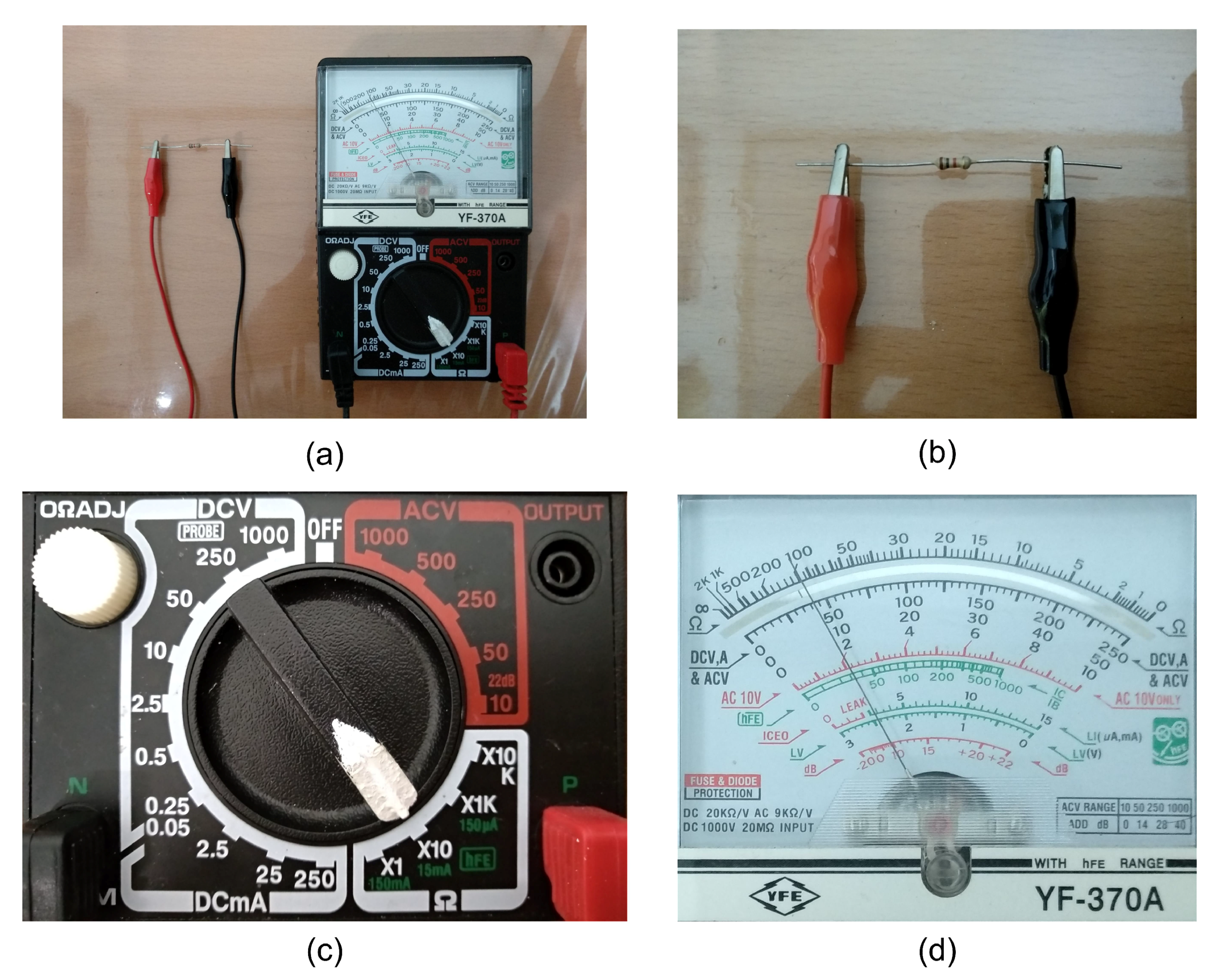
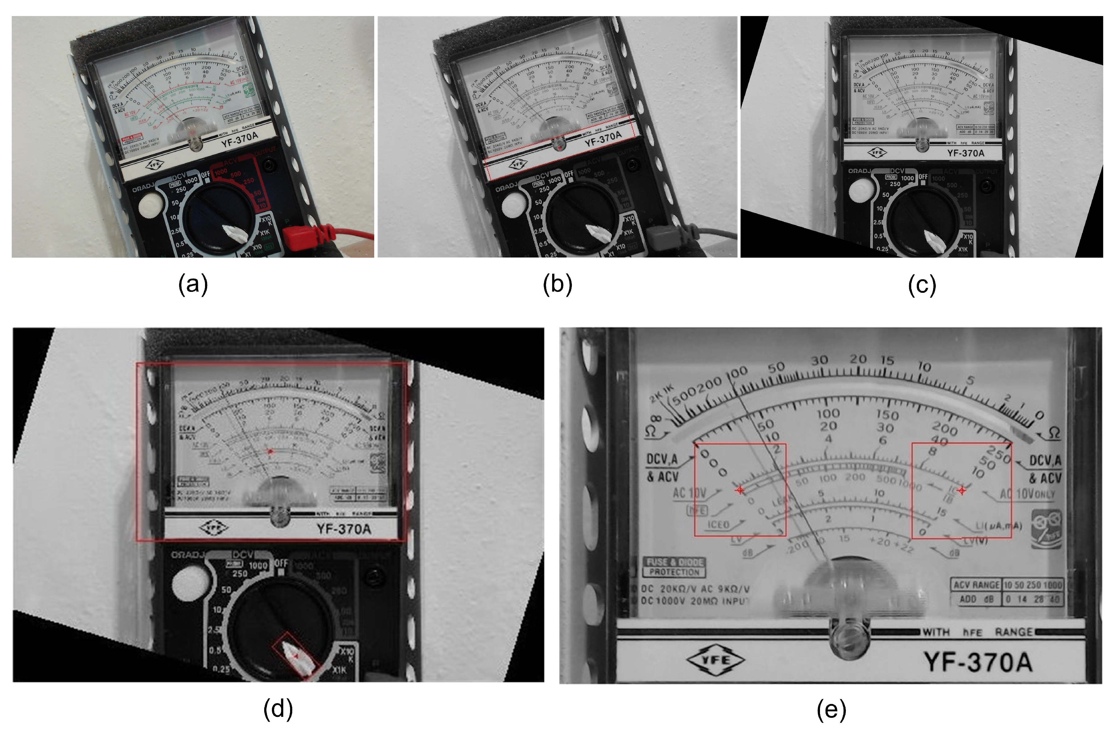
Figure 1a illustrates a scenario where a 1 KΩ resistor is being measured with the A-meter model YF-370A [1], which is used in this study. The 1 KΩ resistor apparently shown in Figure 1b can be identified by the four-band of colors (brown-black-red-gold) which represents (Ω) as studied in reference [2]. According to human operation and visual inspection, in this case, the selector arrow of the function selector is switched to the location of (see also Figure 1c) and the pointer in instrument meter indicates around 100 with the Ω-scale (see also Figure 1d). The resistance about 1000 Ω is thus obtained by (Ω). In fact, the result obtained by human visual inspection is an approximate value due to the viewing angle and the nonlinear Ω-scale, as demonstrated in Figure 1d. Despite such an approximate measurement obtained from an A-meter, from the viewpoint of practical application, it is convenient to let an engineer quickly observe an electronic component characteristic or understand a circuit system’s behavior for instance. According to this philosophy of people using the A-meter, the proposed approach based on computer vision can be simply introduced as follows.
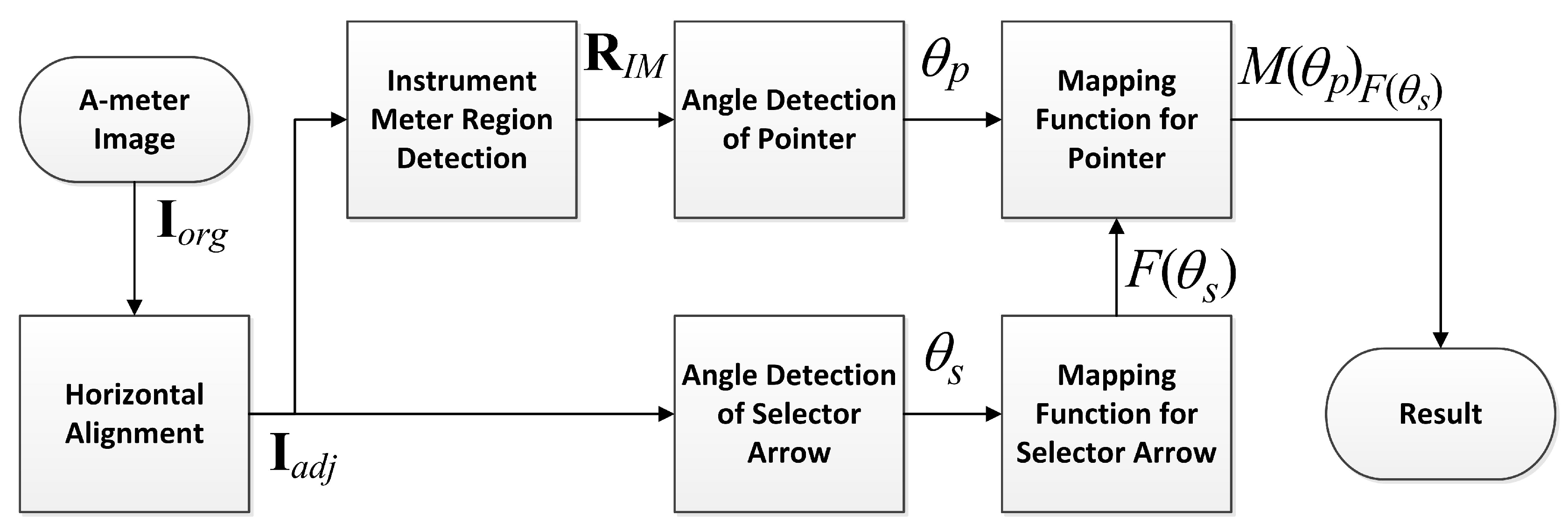
Figure 2 shows the flowchart of our computer vision-based approach. In order to facilitate the effective angle detections in our method, the A-meter image (say original image or ) should be adjusted first in the horizontal orientation using the horizontal alignment stage, and the adjusted image can be obtained as . With the edge-based geometric matching and pyramidal gradient matching techniques, the region of the instrument meter () can then be located by the instrument meter region detection stage. Because the pointer appearing in the is needle-shaped (refer to Figure 1d), the angle () of pointer can be detected at the angle detection of pointer stage. Similarly, the angle () of the selector arrow appearing in the adjusted image can be detected at the angle detection of selector arrow stage. Since reading the A-meter is dependent upon the indications of and , we need two mapping functions, mapping function for selector arrow, , and mapping function for pointer, , to determine which function of the A-meter and which scale in should be used, respectively. Once the is known, the measurement result can then be obtained by .
The related works are simply reviewed in the following text. Several methods have been developed to determine the angle of pointer, where the binary image obtained by image differencing and binarization has often been used for study. For example, in a previous study, two images with different pointer angles were required for image differencing operation to make an instrument meter background image. The background image was used to operate image differencing again with the new position of pointer. Then, binarization and the Hough transform method were used to calculate the pointer angle [3,4]. Guan et al. collected the line intersection points to form a fitting curve which reflected the relationship between the abscissa values and the resistance values [5]. The method proposed by Lima et al. [6] needed the meter to be perfectly horizontally lined up with the camera which would be troublesome for users. Kim et al. described about the automatic recognition of analog and digital meters installed in a nuclear power plant [7]. They applied simple and elementary techniques, such as binarization, region labeling, and projection, to extract needles in analog meters and numeric codes in digital meters. Thresholding was performed to obtain the binary image. Region labeling was applied to extract the image elements. They used a simple run length technique to detect the needle in a meter area and calculated the run length from the center to the edge of the meter image as sweeping circularly. The position with the maximum run length value was selected as the needle position [7]. Li et al. used red light and green light to help detect the pointer for automobile meter calibration and an instrument qualification test before leaving the factory [8]. Zhang et al. studied an improved method of the Hough transform method to detect the pointer angle [9]. Ocampo-Vega et al. used the centroid and tip coordinates of the pointer of a water meter to form a straight line and calculated the pointer angle between the x-axis and the line that was created by joining the tip and the centroid of the pointer [10]. Zhang and Li developed a preprocessing method to automatically read a water meter, where Fourier transform was used to correct a tilted dial image of a water meter [11]. Recently, to develop a Flight Guardian (FG) system which is not physically connected to an aircraft, Khan et al. [12,13] developed a simple method to automatically read the airspeed and revolutions per minute (RPM) of instruments where the video streams are acquired with two fixed-position camera devices. Based on the features of circular shape and needle locations in both dials, the focus of the camera devices is fixed at the center of this shape, and a circular-range sub-image composed of black pixels, except the white pixels occupied by the needle, are adopted for processing. By converting the sub-image pixels into a one-dimensional vector, the needle’s position is identified by finding the maximum convolution output.
In practical applications of automatically reading analog meters, rotated/tilted/shifted situations under variant illumination need to be considered. Based on the research mentioned above, the effectiveness of applying image differencing and binarization methods onto the pointer detection were investigated in the early stages of developing our automatic approach for reading an A-meter, where we found that the useful information lost, as well as the noise yielded, under camera/meter movement or light variation significantly affects the performance of a reading meter. Therefore, in this study, the grayscale images acquired from the A-meter (refer to the , shown in Figure 2), are adopted for algorithm development. Moreover, some techniques are involved in our approach to cope with the situations just mentioned. In order to track a target under variant illumination or a moved situation, a technique to update the template could be helpful [14,15,16,17]. Considering the localization capability under variant illumination and dusky environments, edge-based geometric matching and pyramidal gradient matching techniques are embedded in our approach instead of template updating to localize the wanted regions of interest (ROI) of the A-meter (refer to the main stages of instrument meter region detection, angle detection of pointer as well as angle detection of selector arrow in the flowchart of Figure 2). As a short summary, as depicted in Figure 3, a computer vision system for automatically reading an A-meter is presented in this paper, where the feasibility of our approach is demonstrated by reading the AC voltage, DC voltage, and DC current as well as the resistance value. Here, AC and DC represent “alternating current” and “direct current”, respectively. Inspection by the human eye regarded as a ground truth for comparison and discussion.
The rest of this paper is organized as follows. Section 2 describes the framework and system setup of our study, where the mapping relationship of the function selector and instrument meter are constructed. Moreover, two methods for locating ROIs by template matching as well as the schemes for horizontal alignment of A-meter images and locating the useful ROIs are developed. Section 3 presents the procedure for detecting the pointer’s angle (or position) including the calculation of the pointer’s spin center and a scanning approach to detect the pointer. An illustration is provided in Section 4 to demonstrate the functional behavior of the whole system and confirm the feasibility of our approach. The experimental results and discussion are given in Section 5. Based on a suitable modification of the proposed method, an application to monitor the storage level meter and pressure meter installed on a 15 m liquid nitrogen (LN2) tank is demonstrated in Section 6. The conclusions of this paper and further work related to this study are finally drawn in Section 7.
2. Framework and System Setup
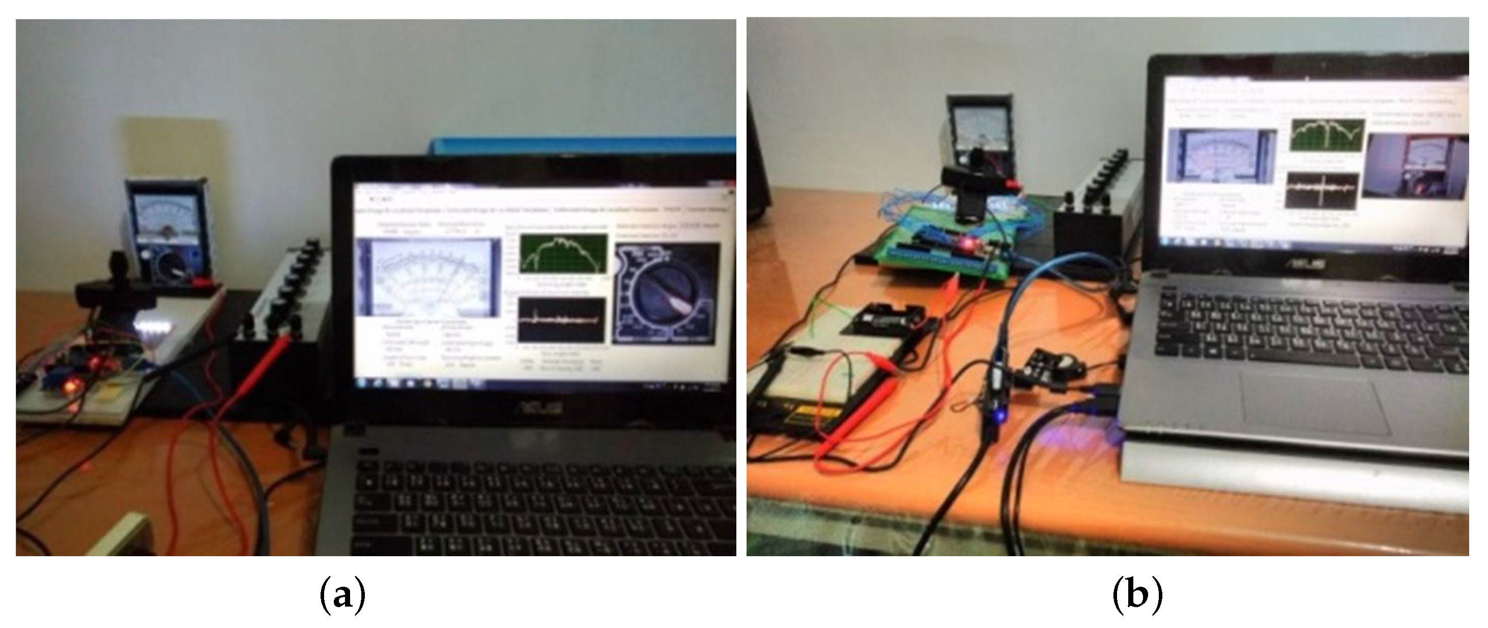
Figure 4 shows our experimental environment including a YF-370A A-meter (Tenmars, Taipei, Taiwan), a C-920 USB camera (Logitech Far East Ltd., Hsinchu, Taiwan), a controllable light source, and a laptop computer. The A-meter image is captured by the USB camera with a size of pixels. The LED light source, used for testing the capability of reading the A-meter under different illuminations, is controlled by an Arduino Mega 2560 microcontroller [18] with its PWM (pulse width modulation) channel. In order to facilitate the system’s integration and build the user interface the proposed algorithms were implemented in a LabVIEW environment [19] combined with the C codes. The capability of reading the A-meter was tested with random orientation under variant illumination and a dusky environment inside a room.
2.1. Mapping Relationship of Function Selector
According to the framework depicted in Figure 3, the sources measured by the A-meter may be the AC voltage, DC voltage, DC current, and resistance. Parts of the system’s setup should be made before the algorithms are developed and experiments conducted, such as the mapping functions used in mapping function for selector arrow and mapping function for pointer, as indicated in Figure 2, as follows. We assumed that the A-meter image was aligned in the horizontal direction. By observing the function selector sub-image illustrated in Figure 1c, the mapping function for the selector arrow was built with the relationship between and . Since there were N functions that were selectable in this A-meter, each function could be identified within a delta range, . Ideally, the i-th function, say , would be indicated with the orientation ∼. However, according to the arrangement of functions in the A-meter, each orientation corresponding a function could be modified within a range, i.e., . Therefore, the index of selected function to be used in mapping function for selector arrow was expressed as
Because there were 20 selectable functions in the illustration presented in Figure 1c, and . Thus, based on Equation (1), the wanted mapping table, , could be expressed as listed in Table 1. Note here that the selected functions for correspond to the linear scales on the instrument meter region (), whereas those for correspond to the nonlinear ones. In order to facilitate the manipulation of reading value from the pointer, an auxiliary value, , is also provided in Table 1, where represents the maximum value used in the functions, (linear cases) and the multiplier used in the functions, (nonlinear cases).
2.2. Mapping Relationship of Instrument Meter
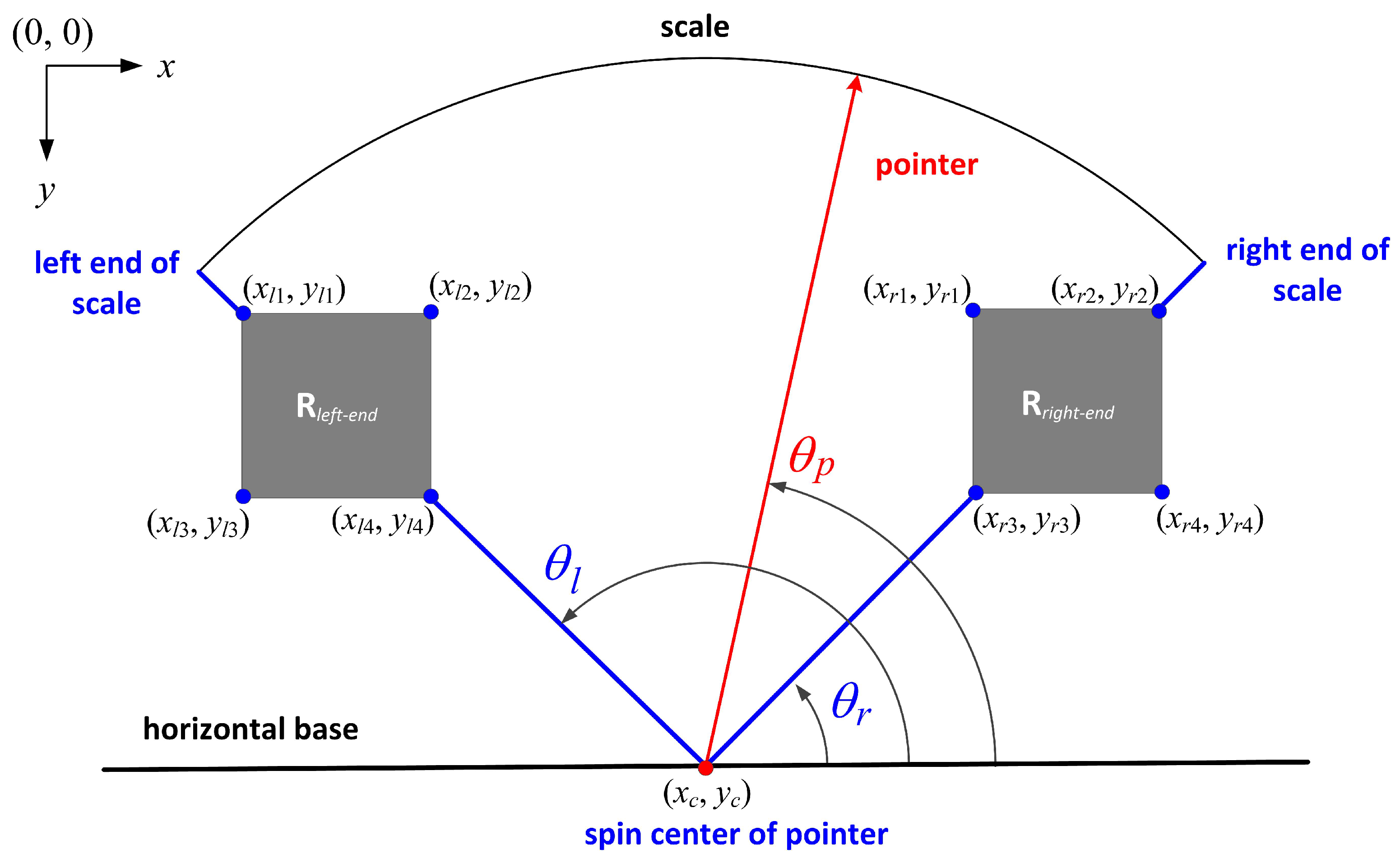
Several scales can be found in the instrument meter sub-image (or ), as illustrated in Figure 1d. In order to correctly read the measured value, we focused on the value indicated by the pointer, ∈, at the scale relative to the selected function in Table 1. The scales in may be arranged in linear (e.g., the scales of ACV, DCV, and DCmA) or nonlinear (e.g., the scale of Ω) form. In addition, they can be designated in sector form, as depicted in Figure 5, where the pointer () with a spin center rotates from right end () to left end (). It was assumed that the A-meter had been adjusted in the horizontal direction. For the linear case, we found that the maximum value, say , was set at the right end of the scale (see Figure 1d for reference). Therefore, the observing or measuring value () from the pointer () could be simply expressed as
If is detected and its in Equation (1) belonged to a linear case, then we had the corresponding maximum value, , in Table 1. Therefore, the above Equation (2) was rewritten as
where in Table 1.
For the nonlinear case, in this study, only the Ω-scale was used, where the maximum value (∞) was located at the left end of the scale, whereas the minimum value (0) was located at the right end. According to the known Ω-scale , as given in Figure 1d, a nonlinear mapping table can be built as listed in Table 2 to solve this situation, where the ground-truth angle, ( in this study) corresponding to the resistance value, , on the Ω-scale can be obtained by means of a protractor. If the pointer was located within two consecutive ground-truth angles, e.g., , the was estimated by interpolation as below
where . If was detected and its in Equation (1) belonged to a nonlinear case, then we had the corresponding multiplier in Table 1. Therefore, the above Equation (4) was rewritten as
where in Table 1.
2.3. Two Methods for Locating ROIs by Template Matching
According to the Equations (1), (3) and (5), it is obvious that the identification of , , , and are based on a horizontally aligned A-meter and can be achieved with the template matching scheme. Therefore, several fundamental templates were built in prior and used in our approach. To perform the template matching, the edge-based geometric matching and pyramidal gradient matching techniques were adopted in our system. Edge-based geometric matching uses the curves obtained from the edge information of a template image as the basis for the features that are used for matching. Pyramidal gradient matching is able to reduce the size of the image and the template to improve the accuracy and the execution time of pattern matching as well as to increase the performance of matching the blur or low contrast image. The edge information was used in both of the two algorithms. Since the algorithms for edge-based geometric matching (EGM) and pyramidal gradient matching (PGM) have been widely used and embedded in the NI (National Instruments) vision software for machine vision applications [21] and for LabVIEW [19], we do not review their principles here, but we applied them into our approach with the following expressions. Let be an input image and denote the template, which will be introduced later, for matching process. Both and are grayscale images. The return result of each matching includes three elements, i.e., flag, ROI, and rotation, and can be formulated as
and
where flag denotes the matching successes (1) or not (0). ROI represents the four coordinates of the located region if flag is 1. In addition, since the functions of EGM and PGM can deal with the rotation cases, the parameter rotation reflects the rotation angle of the located ROI if the flag is 1.
2.4. Horizontal Alignment of an A-Meter Image
For the flowchart designated in Figure 2 to read an A-meter (), the horizontal alignment is the first step to adjust into for further processing. In this study, the EGM method expressed in Equation (6) was used for horizontal alignment where the input image was the original A-meter image () and one useful middle part of the A-meter shown in Figure 6 is used as the template for matching. Thus, the Equation (6) may be expressed by
Once the and were detected, the horizontally adjusted image was obtained by rotating the about the center of the located minus the .
2.5. Locating the Useful ROIs
After obtaining the , some ROIs were located in order to compute the pointer angle, , as indicated in Figure 2, where the was located first. Because the , including the pointer and scale details, is of great importance in this study, both the EGM and PGM methods were applied for template matching to increase the correctness of locating from the image, . In addition, in order to compute the right end () and the left end () of the scale, , as indicated in Figure 5, the right end ROI and left end ROI also needed to be located carefully. Therefore, both the EGM and PGM methods were also applied to locate the and . That is, to locate the ROI’s , and , the designated approach was the same and was unified as follows. For each case, two kinds of templates, namely and , were adopted for template matching and used in the EGM and PGM methods, respectively. In order to let our method cope with a reasonable matching range from a bright to dark situation, two templates, and , were built for the PGM method. or was chosen and used in the PGM based on the mean intensity () of the given input image I and may be expressed by
In this study, the threshold (TH = 52) was heuristically selected and used in our experiments. Accordingly, in order to locate the ROI R with both EGM and PGM methods, the Equations (6) and (7) were rewritten respectively as below
and
If both methods successfully located an ROI for R, the one with a smaller rotation angle was the desired ROI, since its position would be closer to the horizontal base (). Thus, the located R was finally determined by the following expression,
Based on the Equations from (9) to (12), the used templates are listed and shown in Figure 7 to locate the , and . Figure 7a–c show the templates (, and ) used to locate . Figure 7d–f show the templates (, and ) used to locate . Figure 7g–i shows the templates (, and ) used to locate . In Equations (10) and (11), to find , the input image was , whereas to find and , the input image was . The notations are summarized in Table 3 to locate the , , and .
By following the method presented in Section 2.4, the information to locate the selector arrow () was also found with the PGM method using the given template (), as shown in Figure 8, which may be expressed as below. In this situation, the image was used for matching.
Note here that the located is ignored but the rotation is used and is just the wanted as noted in Section 2.1. That is, .
3. Angle Detection of Pointer
3.1. Spin Center Calculation of Pointer
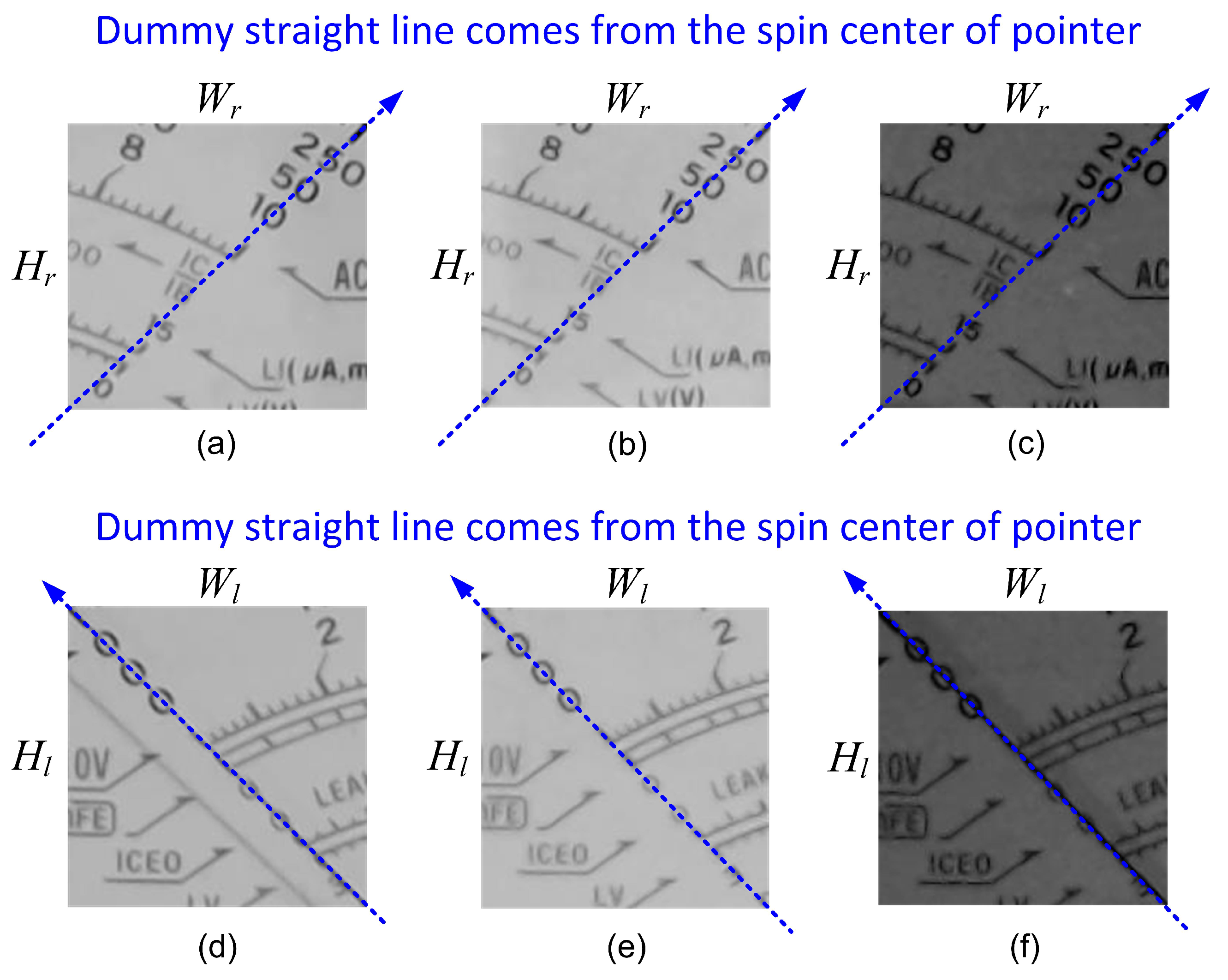
Based on the located and in presented in Section 2.5, the relationship between the pointer indicated by and the scale in (refer to Figure 5) were replotted by adding the coordinates {, , , } of and {, , , } of , as depicted in Figure 9. In this study, the templates for the right-end scale, i.e., , and , given respectively in Figure 7d–f, were selected with a rectangular ROI so that one pair of diagonal corner points were just passed over by a dummy straight line of the right-end scale (from the spin center of pointer) as redrawn in Figure 10a–c. Therefore, the angle of the right-end of the scale ( in degrees) was expressed by
Similarly, the templates for the left-end scale, i.e., , and , given respectively in Figure 7g–i, were selected with a rectangular ROI so that one pair of diagonal corner points were just passed over by a dummy straight line of the left-end scale (comes from the spin center of pointer), as redrawn in Figure 10d–f. Therefore, the angle of the left-end of the scale ( in degrees) was expressed by
In the current study on the YF-370A A-meter, because of and , we thus had and . These matched with the ground-truth angles, i.e., and , as listed in Table 2, which were obtained by means of a protractor. By reconsidering the illustration given in Figure 9, once the and were located, the Equations (14) and (15) could be rewritten as
and
In addition, by observing the Figure 9, the straight line of right end of scale was shown to pass approximately over and and the left-end of the scale passed approximately over and . By solving the two line equations joining one point, the spin center of pointer was thus obtained by the following expressions
Note here that the origin (0, 0) is the top-left coordinate of the image.
3.2. Scanning Approach to Detect the Pointer
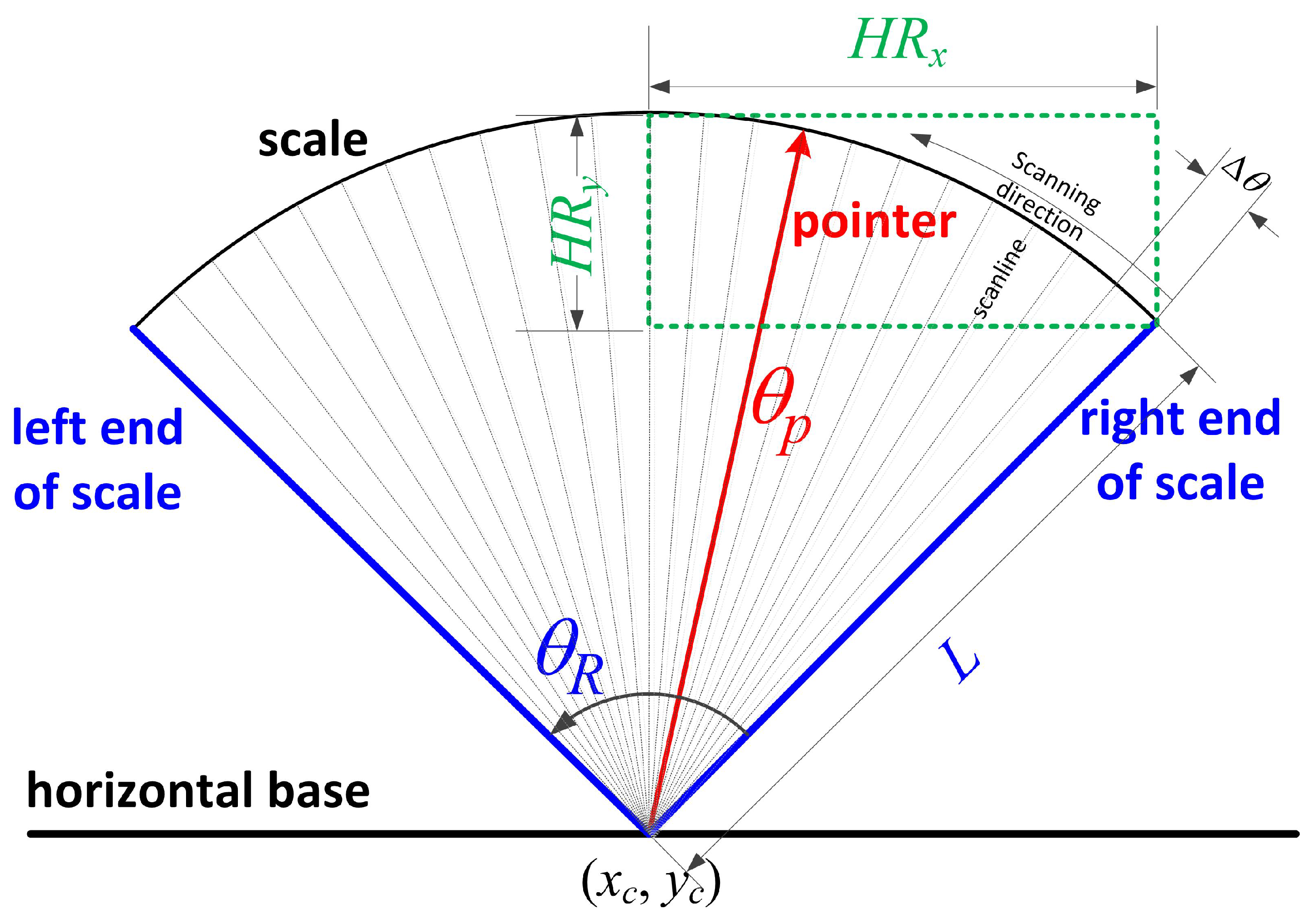
The traditional projection scheme was borrowed here to detect the pointer. Our approach was to scan the image () with a scanline (which has a length, L) about the spin center from to , as illustrated in Figure 11 so that all pixels within the sector region were visited once at least by the scan. Thus, the scan step () was selected carefully and is presented later in this section. Here, L can be determined by the distance between and (or ), i.e., , as illustrated in Figure 9. In this study, the extent () was set heuristically to 15 for our experiments. The method was as follows: Let be the set of all pixels belonging to the i-th scanline, and represent the corresponding -value of the i-th scanline. In addition, let be the image intensity (or grayscale value) of the pixel (p). Therefore, the accumulation of all pixels’ intensities within the i-th scanline, , otherwise known as the A-quantity, was expressed as
Ideally, since the appearance of the pointer tends to be a dark color, the pointer indicated by the k-th scanline should possess the lowest accumulation value, , and the pointer’s angle () is intuitively the corresponding . However, this detection rule can fail due to the very thin pointer as well as the interferences of characters and the pointer’s shadow on the meter surface. In order to enhance the detection correctness, the gradient of was further derived as or called the profile of . Since along the scanning direction, the A-quantity of the thin pointer and its one neighbor may be changed from a large amount to a small amount or from a small amount to a large amount, the pointer’s position indicated by the k-th scanline should possess the largest change with zero-crossing property, where the sign of and that of are mutually opposite. The pointer’s angle was thus detected and expressed by
Referring to Figure 11 in order to perform effectively the scanning process, the incremental amount of scanning degree for each step needed to be determined so that the total number of scanning steps with in the image domain was satisfied but not redundant. The following method was used: Let the changing amount in the horizontal and vertical directionswith the scanning range () be a full range of and , respectively. Theoretically, the larger one between and will dominate the so that there are more scanlines to cover all the pixels within the sector region with the during the scanning process. This was expressed by
As shown in the illustration in Figure 11, and can be replaced by double half range and , respectively. That is, and . Using trigonometric expressions, and may be expressed by
and
Note here that since the pointer may be located at the right end () or the left end () of the scale, to detect the pointer, the scanning range needs to be wider than in real applications. Therefore, we heuristically set to be the starting position and to be the ending position for our scanning process, where the pointer’s angle was found with Equation (20).
4. Illustration of Reading the A-Meter
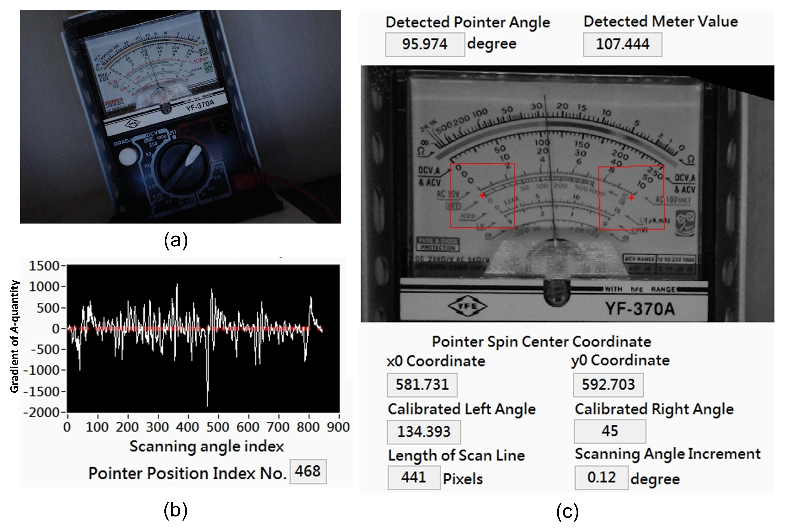
After presenting the methodology of our approach with the framework and system setup in Section 2 and the angle detection of pointer in Section 3, a series of results of measuring a 1KΩ resistor by the A-meter YF-370A are shown here to demonstrate the feasibility of the proposed approach. Figure 12a shows the original image (), where one 1KΩ resistor is being measured by an A-meter YF-370A. The gray channel of Figure 12a was used for further processing, where its mean intensity was . By template matching using Equation (8) with the template () given in Figure 6, was detected, where the center of was (1225.9, 1420.6), as depicted in Figure 12b. Then, the horizontal alignment image () was obtained by rotating the in Figure 12a about the center (1225.9, 1420.6) with , as shown in Figure 12c.
Next, by performing template matching using Equation (12) with the templates given in Figure 7a–c onto the , the was located as the top region marked with the red rectangle in Figure 12d, where the selector arrow was also found using Equation (13), with the template given in Figure 8. The was used later for the detection of the right-end and left-end of the scale. In this step, the detected selector arrow reported the rotation angle as . According to Equation (1) and the mapping table in Table 1, this indicates that the current selection represents the function name “”; a nonlinear case; and is a multiplier.
Within the found , Figure 12e shows that the useful right-end and left-end of the scale were obtained by means of Equation (12) with the templates given in Figure 7d–f and Figure 7g–i, respectively. In this step, the coordinates of were found by , , , and , and those of were found by , , , and . Therefore, according to Equation (16) and according to Equation (17), respectively. In addition, by means of Equation (18), the spin center was obtained as .
According to the results obtained above, we the scanline length (pixels) and , based on Equation (21), were used in our scanning process to detect the . As noted in Section 3.2, to detect the pointer, the scanning range needed to be wider than in real applications. Thus, the process was scanned from to to produce the accumulation profile of A and the gradient profile of , as shown in Figure 13a,b, respectively. In this example, itwo valleys obviously appeared (Figure 13a), which indicated the positions of and , respectively. From the GA-profile in Figure 13b and according to Equation (20), the detected index was with the corresponding , which was just the detected pointer’s position () in the current illustration.
Based on and the selector function “” with the multiplier , Table 2 and Equation (5) were used to determine the , i.e., the resistance of the measured 1KΩ resistor. From Table 2, since , we had , , , and . Using the computation of Equation (5), a resistance of was obtained which is very close to 1 KΩ. Thus, the feasibility of the proposed approach is confirmed.
5. Results and Discussions
In order to further demonstrate the effectiveness of the proposed approach to read an A-meter, the often used functions—reading the AC voltage, DC voltage, and DC current as well as resistance values—were adopted for experiments and evaluations. Since there is no true value for reading a measurement from the A-meter, in this study, inspection by the human eye was regarded as the ground truth for evaluating the accuracy of the proposed method as the framework given in Figure 3. is the value from the A-meter read by human eyes, and is that read by the proposed method. The accuracy (%) was defined as
and was used for the performance evaluation. With the A-meter YF-370A, there were 15 experimental scenarios that were designated as follows.
- (1)
- function select “OFF”.
- (2)
- function select “ACV 250” to measure the 110 Vac line power.
- (3)
- function select “ACV 250” to measure the 220 Vac line power.
- (4)
- function select “DCV 2.5” to measure the 1.5 Vdc battery.
- (5)
- function select “DCV 10” to measure the 5 Vdc adaptor.
- (6)
- function select “DCV 10” to measure the 7.5 Vdc adaptor.
- (7)
- function select “DCV 10” to measure the 9 Vdc battery.
- (8)
- function select “DCV 50” to measure the 12 Vdc adaptor.
- (9)
- function select “DCV 50” to measure the 24 Vdc adaptor.
- (10)
- function select “DCmA 25” to measure the DC current of 1.5 V battery.
- (11)
- function select “” to measure the resistance of 50 Ω.
- (12)
- function select “” to measure the resistance of 220 Ω.
- (13)
- function select “” to measure the resistance of 1 KΩ.
- (14)
- function select “ 1 K” to measure the resistance of 1 KΩ.
- (15)
- function select “ 10 K” to measure the resistance of 70 KΩ.
Scenarios (1)–(10) belong to the linear cases and their results are presented in Section 5.1. Scenarios (11)–(15) belong to the nonlinear cases and their results are presented in Section 5.2. Section 5.3 further discusses the influence of illumination to the proposed approach and uses a digital meter instead of human eyes to reconfirm the accuracy of the proposed method. In addition, the influences of translation and/or rotation as well as the effective range of using our approach are also investigated.
5.1. Experimental Results on Linear Cases
In order to test the feasibility of our method under different rotations () and illuminations (mean intensity ) of the A-meter YF-370A, five measurements for each scenario were performed by human eyes and the proposed approach and were analysed and compared. We checked the function select () detected and the read value () obtained by human eyes and those ( and ) by the proposed method, respectively and then evaluated the accuracy with Equation (24). Note here that if the signs of were positive, it meant that the A-meter was rotated to the left; otherwise it was rotated to the right. In addition, the lower the was, the darker the illumination was, and vice versa.
The first scenario (1) was to let function select be “OFF”, where the measurement resulted in 100% accuracy, as reported in Table 4. This means that the rotated A-meter was horizontally adjusted, and the function select and the meter pointer were detected correctly for each case by the proposed method. Note here that since both and were 0, they were identical and Equation (24) was not needed.
For scenario (2), the A-meter was set to function “ACV 250” to measure the 110Vac line power. Table 5 reports the mean accuracy as 97.28%. Note here that the second row is a slightly tilted case with low illumination, as shown in Figure 14. In this tilted example, represents that the function “ACV 250” was selected and was used according to Equation (1) and Table 1, where implies that this example is a linear case. In addition, , were obtained respectively by Equations (16) and (17) using the detected and , as detected in Figure 14c. Through our scanning process (using ) on the GA-profile as shown in Figure 14b, was thus detected. Since the current example is a linear case, Equation (3) was used and the read result Vac was finally obtained. Even the A-meter was rotated 15.947 and the illumination was low: . In this case, the result Vac obtained by the proposed method is very close to the Vac observed by human eyes. Table 6 reports the results for scenario (3), where the function “ACV 250” was also selected to measure the 220Vac line power. The mean accuracy was 98.86% except for the fifth data point, since it was difficult to read by the human eye (but our system read the value as 236.450 Vac) under very low illumination ().
The results of the other linear cases (scenarios (4)–(10)) using function selects of “DCV 2.5”, “DCV 10”, “DCV 50” as well as “DCmA 25” are reported in Table 7. From these experimental results, it is shown that all of the function selects were detected with 100% accuracy. The pointer was detected very accurately and the mean accuracy of the reading value for most of cases was 95% or above.
5.2. Experimental Results on Nonlinear Cases
In this study, the nonlinear scale merely considered the resistance measurement with the A-meter YF-370A. The DC resistance controller ZX99A [20], as shown in Figure 15, was used to provide the reference resistance for our experiments. The results of the nonlinear cases (scenarios (11)–(15)) of using function selects of “”, “ 1 K”, and “ 10 K” are reported respectively in Table 8. From these experimental results, all the function selects were detected with 100% accuracy. The pointer was detected very well and the mean accuracy of the reading value for most of cases was above 97% except for the case using “ K” to measure the 1 KΩ resistor reported in Table 8d, where the mean accuracy was 87.27%. By observing the nonlinear scale on the meter surface, as shown in Figure 1d, it appears that it this accuracy decay for the function select “ 1 K” to measure the 1 KΩ resistor was reasonable since a little difference around “1” may result in a large change due to the large multiplier “” (we call it the little-change-large-multiplier effect). Contrarily, the phenomenon was reduced using the function select “” to measure the 1 KΩ resistor (refer to Table 8c) since the value around “100” indicated by the pointer is greater than that around “1”, and the multiplier of “” is less than that of “”.
5.3. Further Results and Discussion
So far the proposed approach has been confirmed by experiments using both linear cases and nonlinear cases, as presented in Section 5.1 and Section 5.2, respectively. In these experiments, in addition to obviously rotating the A-meter, we also randomly set the A-meter to be slightly tilted and adjusted the illumination from dark to bright during the experimental period where the illumination controlled by the LED of our system was reflected by the mean intensity of . An experiment was further conducted as follows to verify the usable range of . The A-meter YF-370A was rotated by 15.425 and the 110 Vac line power was measured with function select “ACV 250”. Table 9 reports that the proposed method can perform very well as long as the mean intensity is .
The performance evaluations of those experiments presented previously were based on inspection by the human eye (), where looking at the A-meter (or viewing angle) will result in an error due to reading the value indicated by the pointer. Similarly, such a situation (like the “tilted surface” noted in the previous experiments) will also appear in our computer vision-based approach. Hence, it can be concluded that the errors resulting from the A-meter itself and the observation from human eyes or a vision sensor are inevitable under the scenario of using an A-meter. In order to further confirm the feasibility of the proposed method, a digital multimeter (model DMM-85) instead of human eyes was used to read the value of measurement as ground truth (). By replacing by , Equation (24) was also used for the accuracy evaluation. Table 10 reports that a mean accuracy of 95.61% can be achieved. Note here that the little-change-large-multiplier effect appears in the experiment of the last row of Table 10, where the accuracy decayed to 88.77%.
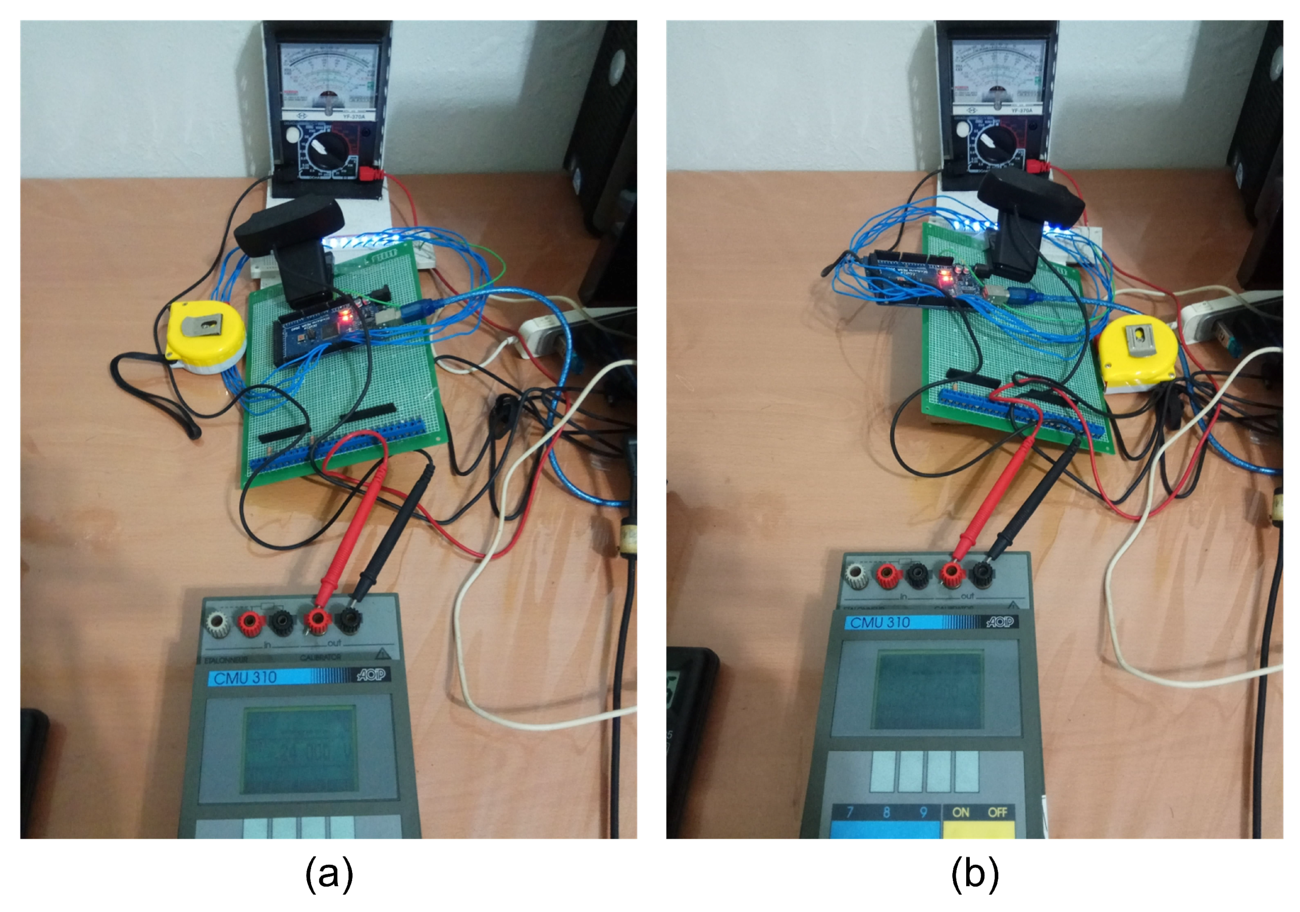
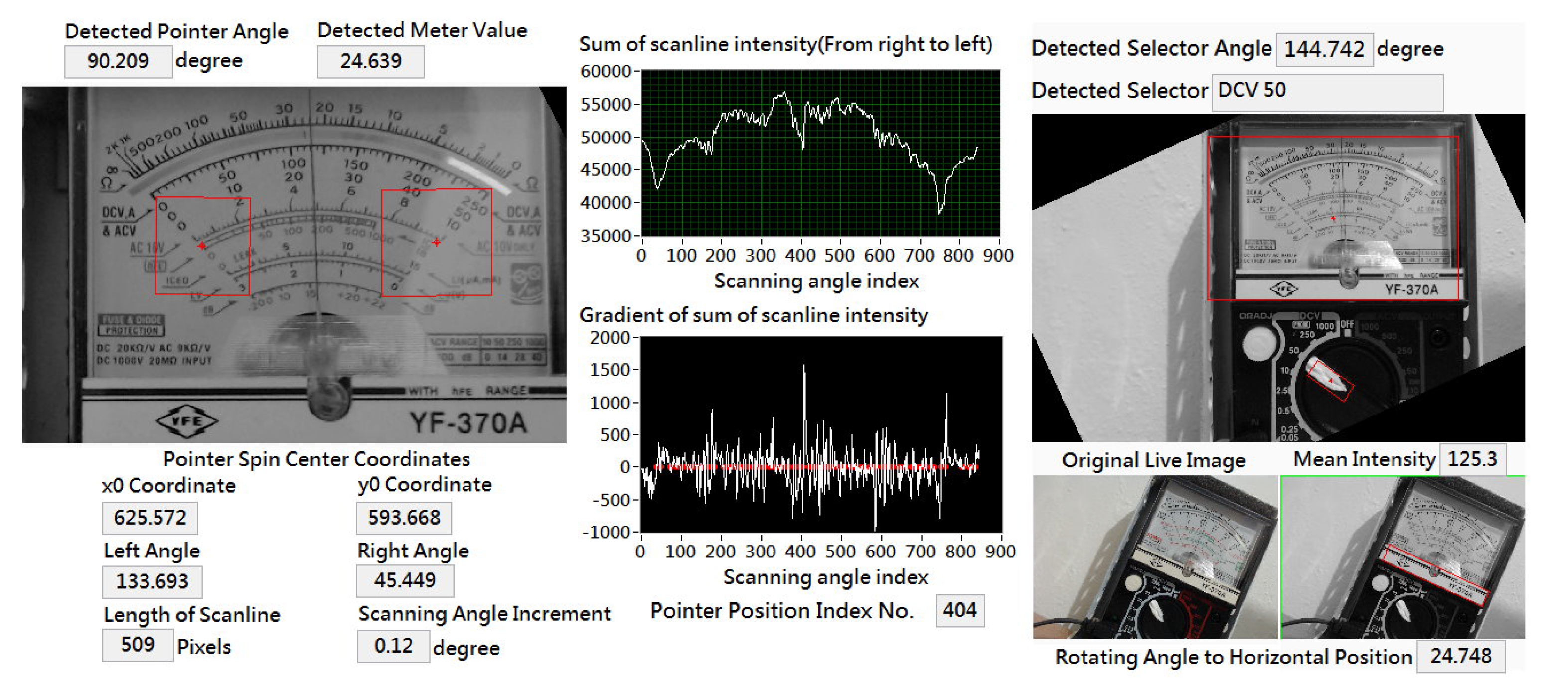
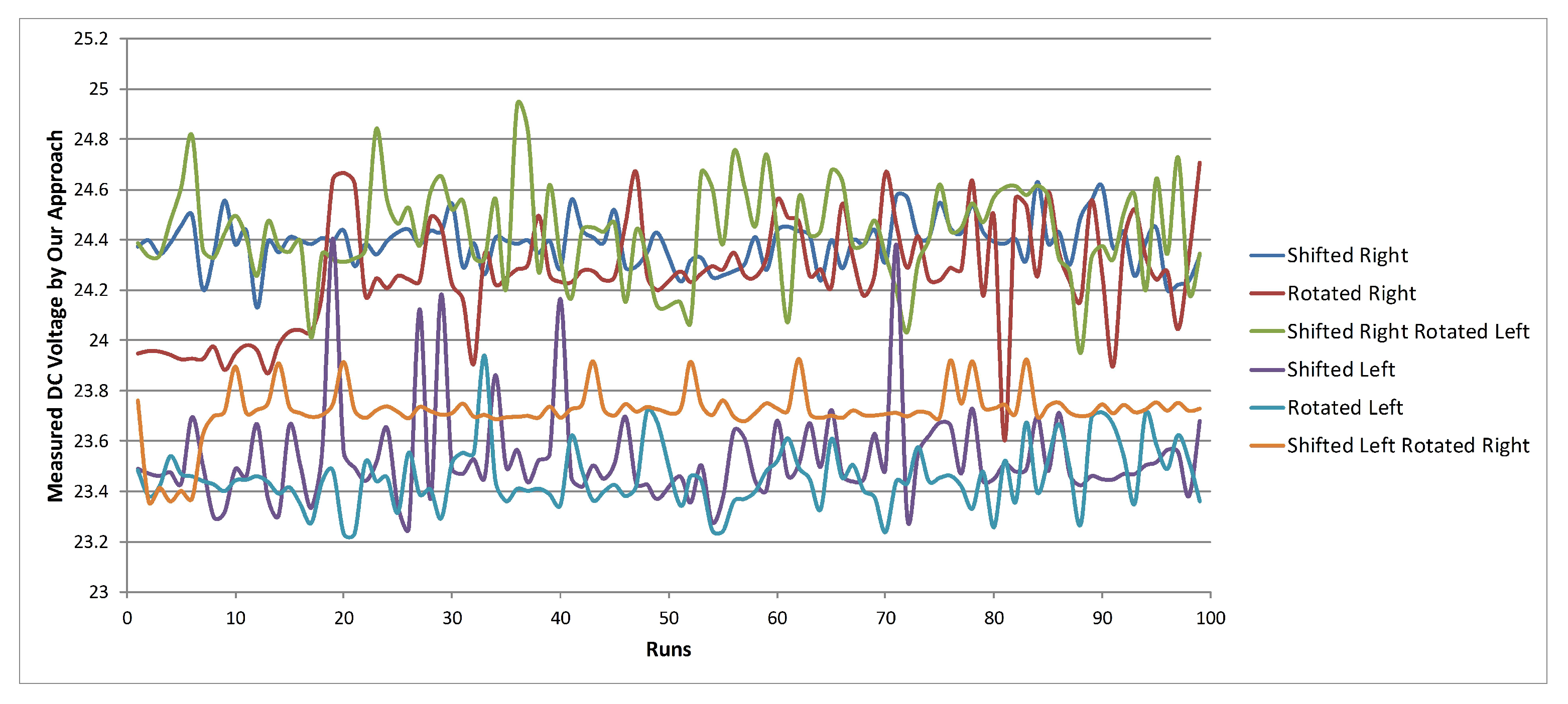
To investigate the influences of translation and/or rotation using our approach, we experimented with shifting and/or rotating the camera of our system to read the A-meter. The tester calibrator (model AOIP CMU 310) was used to provide a stable 24 Vdc as the ground truth and the function of the A-meter was switched to “DC 50V” for the experiments. Six scenarios were designated as the A-meter in the captured image: (1) shifted right, (2) rotated right, (3) shifted right and rotated left, (4) shifted left, (5) rotated left, and (6) shifted left and rotated right, where scenarios (2) and (5) were obtained by the arrangements shown in Figure 16a,b, and their illustrative results are presented in Figure 17 and Figure 18, respectively. In this experiment, there were 100 consecutive runs for each scenario in our approach. The measured DC voltages for the six scenarios are plotted in Figure 19, and their statistical results are reported in Table 11. The plots shown in Figure 19, demonstrate that a slight fluctuation existed when reading the A-meter using our computer vision-based system. In addition, as reported in Table 11, when the camera was located at the left-side relative to the A-meter (e.g., scenarios (1)–(3)), the reading value was higher than 24 Vdc, and vice versa (e.g., scenarios (4)–(6)). This matches with the relationship among the observer, needle, and scale along a line of sight. Note here that the lowest value (0) of the “DC 50V” scale on the A-meter was located at the left-end, whereas the highest value (50) was located at the right-end (see Figure 17 and Figure 18 for reference).Even though the recognition value produced by our system was not always as stable as the digital value displayed in the tester calibrator, a mean accuracy of around 98% was still able to be achieved. As a short conclusion, an “uncertainty problem” exists when obtaining measurement values from an analog meter. Two obvious uncertainties can be observed during the measuring process. First, since the measurement value is indicated by rotating a needle-type pointer onto a marked scale, an error will result from the mechanical rotation, the quality of the pointer, and the scale. Secondly, viewing directly onto the meter by not only the human eye or a camera will also lead to a reading error as the experimental results showed.
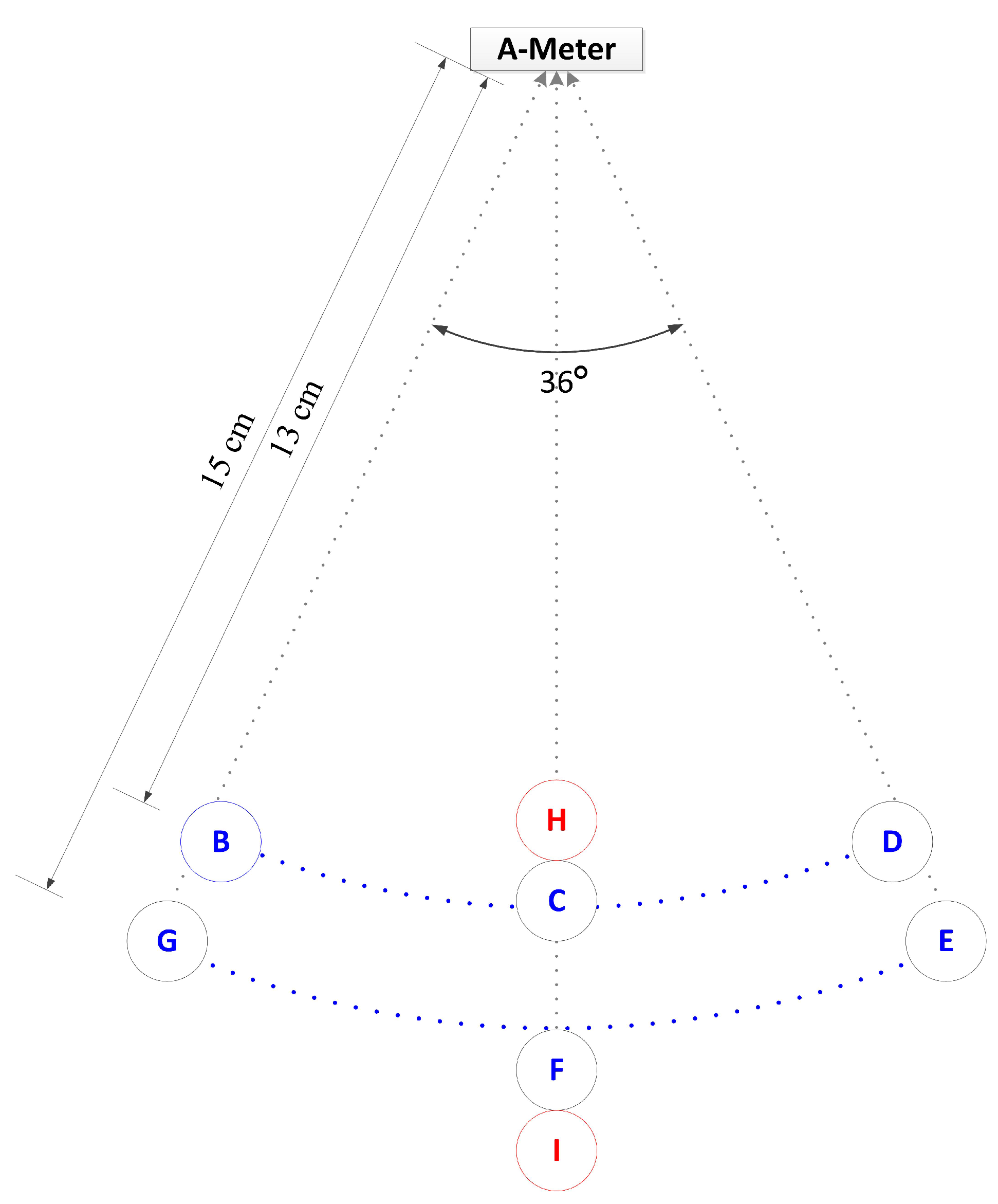
Because the location of the ROIs in our approach was based on template matching, as presented in Section 2.3, the fundamental templates needed to be trained and built in prior. Even though the adopted templates are fixed and limited in the current system, based on the previous experiment, it was determined that it was worth conducting another experiment to examine the rough effective range. Again, the tester calibrator (model AOIP CMU 310) was used to provide a stable 24 Vdc as ground truth and the function of A-meter was switched to “DCV 50” for experiments. We moved the camera to read the A-meter and examine the effective result repeatedly. Finally, an effective range, as drawn in Figure 20, was obtained, namely, it was determined that the camera should be placed at a location about 13∼15 cm distance from the A-meter and the viewing orientation should be within about the center line. Note here that F has a distance from the A-meter of 16 cm; in this case, our system still can function well. The statistical results reported in Table 12 confirm that our computer vision-based approach can allow the A-meter to be read within the effective range drawn in Figure 20. If the camera is placed outside the effective region, reading the A-meter will fail. For example, consider the H and I in Figure 20. H and I have distances of 12 cm and 17 cm from the A-meter, respectively, and represent the camera being placed outside the effective range. Their experimental results displayed in Figure 21 and Figure 22, respectively show that they fail to read the A-meter. As a comment, the scalability of the current system will depend on the A-meter included in the processed image, the resolution of the image, as well as the set of templates to be trained.
Currently, the proposed algorithms are implemented in the LabVIEW environment [19] by combining with the C codes and plotting the visualized results for functional verification only. The execution time still bounds in the “second” level with an image size of pixels for processing. Most of the time is spent on template matching and horizontal alignment. It takes about 90% of the whole execution time in the current implementation. The time taken to detect the pointer and read the value takes around 1 s, as the videos demonstrate in reference [22,23]. The first video [22] shows the stability of locating the and the and reading the value. The second video [23] demonstrates the scanning process to detect the pointer and read the value. Based on the effectiveness of reading the A-meter with the presented method, an application to read the dials attached on a liquid nitrogen tank is further demonstrated in the next section.
As a result, the computer vision-based approach has been proposed to effectively read the value on not only the linear scale but also on the nonlinear scale indicated by the pointer from an analog multimeter. Through a comparison of the results obtained by the proposed method to those obtained by both human eyes and the digital multimeter, our experiments confirmed that the accuracy of locating the function select is 100%, and the mean accuracy of reading the value from the A-meter is 95% or above ,except for some cases affected by the little-change-large-multiplier effect. Our method was also shown to perform well under situations where the A-meter is rotated, slightly tilted, and/or illumination varied and thus, its feasibility and effectiveness are confirmed.
6. Application of Monitoring Liquid Nitrogen Meters
By suitably modifying our algorithms, the proposed approach can be applied for reading the similar kinds of A-meters. In this section, we demonstrate a successful application of monitoring a storage level meter and pressure meter installed on a 15 m liquid nitrogen (LN2) tank which is located at outside our laboratory, as shown in Figure 23a. These two analog needle-type meters are very significant for our laboratory and need to be checked frequently to guarantee that the storage level and pressure of tank are maintained within a safe range. For example, excessive pressure will damage the solenoid valve of testing equipment and cause other dangerous situations, and once the LN2 storage level is below the low limit, the technician should call for LN2 filling to avoid sudden interruption of testing in laboratory. Reading such an analog meter based on human eyes is rather inefficient and will easily cause fatigue problems during long-term monitoring. Therefore, our computer vision approach is a valuable way to deal with such a scenario.
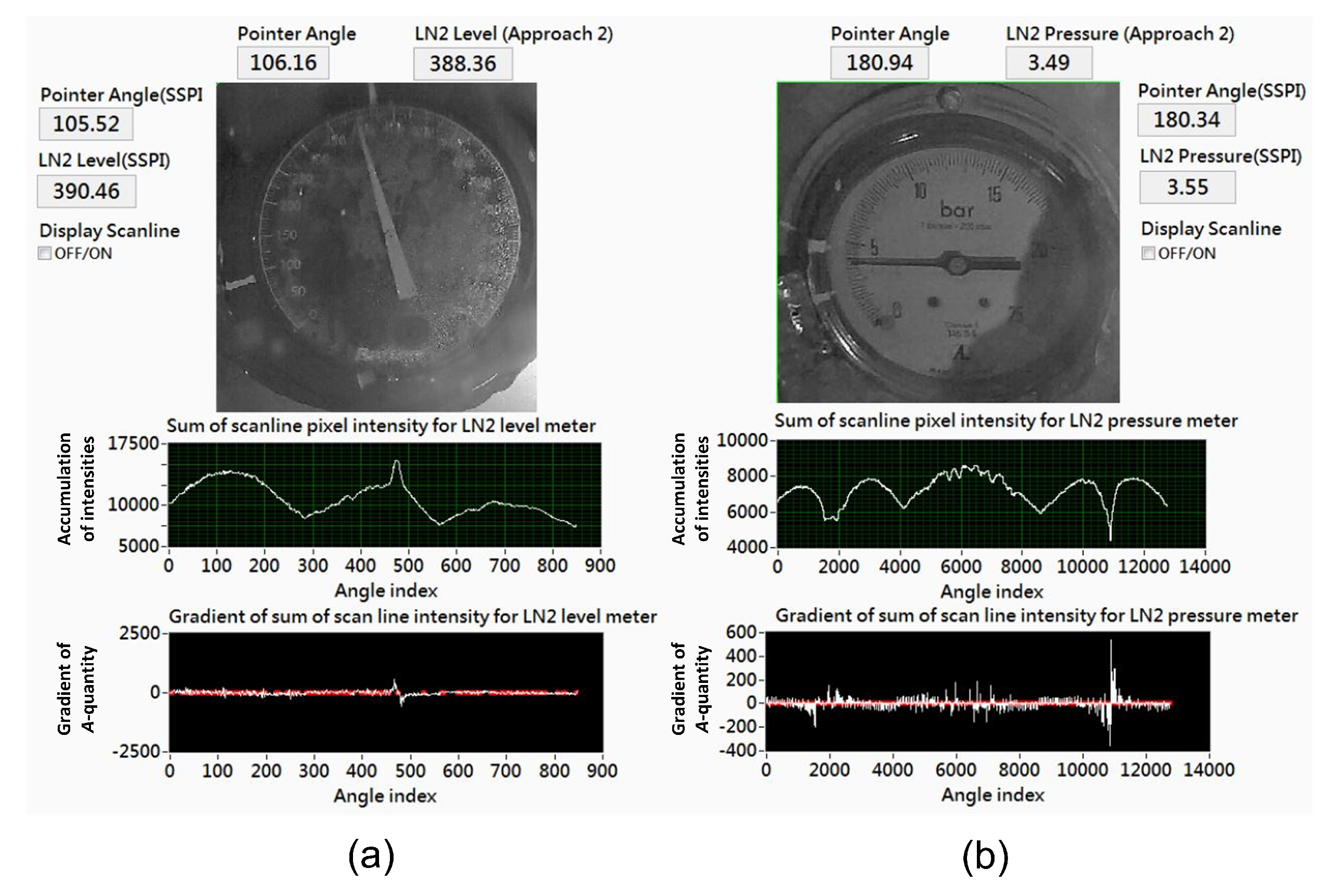
In this application, an Internet Protocol (IP) camera (model AXIS P3364-LVE 12mm [24]) was installed to acquire the video stream (with a frame resolution of pixels and frame rate 30 frames/sec) including both the level and pressure meters, as shown in Figure 23b. At night, the LN2 tank meters can be illuminated by a road lamp and a LED flood light as shown in Figure 23c. For each frame, the subimage of the level meter and pressure meter is extracted first according to the predefined ROIs, and then processed individually by our method to read the value indicated by the meter pointer. Note here that only the pointer’s angle detection (presented in Section 3) was implemented in this application. Figure 24 illustrates one frame containing the level and pressure meters from a video stream at rainy night. Using our monitoring system, the results shown in Figure 25 demonstrate the usefulness of our method in this application. Even during worst-case scenarios, such as rainy nights, our system can work well, as shown by the results in Figure 26.
Since the storage level of LN2 gradually decreases during consumption in the laboratory and increases during filling, the pointers shown on the two meters normally vary very slowly, as the real video (recorded in rainy day) demonstrated in [25], and the pressure should be maintained within a range between 3 to 5 bar, and the storage of LN2 should be maintained above 80, as indicated on the scale used by our laboratory. In order to show the capability of reading the LN2 meters by our method, we intentionally set the pointer of meter moving fast by manual as the real video demonstrated in [26]. The two videos given in [25,26] demonstrate that our system can read the two dials on the LN2 tank in a real application with an execution time of about 0.2∼0.6 s for each reading. This can be regarded as real-time processing, compared to the very slow change of the meter pointer. As a result, such a non-invasive computer vision system provides us a convenient alternative to monitor the LN2 tank information without installing additional expensive digital sensors and truly helps us to guarantee the safety of using LN2.
7. Conclusions and Future Work
The analog multimeter (A-meter) is a significant instrument for sensing or measuring electronic signals, e.g., voltage, current, resistance, and so on. Even though the digital multimeter is commonly used in our daily life under the considerations of precision and cost, the analog multimeter is still a preferable device for many applications due to its ability to monitor promptly varying values. In order to retain the merits of A-meter and to reduce the tiredness of human eyes observing the A-meter over long durations, it is of great importance to develop a computer vision-based method to automatically read the measured value indicated by the pointer of the A-meter. To effectively read an A-meter, the presented algorithms include horizontal alignment of the A-meter, detection of the instrument meter region, angle detection of the selector arrow, and angle detection of the pointer. The desired ROIs used in our algorithms are extracted by two template matching methods—edge-based geometric matching (EGM) and pyramidal gradient matching (PGM)—which have been widely used and embedded in the NI vision software for machine vision applications [21] and for LabVIEW [19]. Moreover, the mapping relationship between the function selector and the selector arrow, as well as that between the instrument meter and the pointer are built and formulated to read the A-meter, where the scale on the meter may be linear or nonlinear. The often used scenarios of reading AC voltage, DC voltage, and DC current as well as resistance were adopted for the experiments and evaluations in this study. Our experimental results showed that using our method, the accuracy of detecting the function select was 100%, and the mean accuracy of reading values from the A-meter was 95% or above, except for some cases of reading resistance affected by the so-called little-change-large-multiplier effect. In addition, the proposed method performed very well as long as the mean intensity, i.e., illumination was . The “uncertainty problem” in reading an analog meter was explored using translation and/or rotation of the camera to read the A-meter by the proposed computer vision-based approach. The effective range to use our method within was also investigated and validated. Based on suitable modification of the proposed method, an application involving the monitoring of a storage level meter and pressure meter installed on a 15 m liquid nitrogen (LN2) tank was demonstrated successfully. In conclusion, even if the A-meter is rotated, slightly tilted and/or illumination varied, the proposed computer vision-based approach can effectively read the analog multimeter. A general purpose method for reading the A-meter, its real-time implementation and a time complexity analysis, as well as a more deep investigation on the uncertainty issue are worthy of further study and could be regarded as our future works.
Author Contributions
Conceptualization, Y.-S.C.; Data curation, J.-Y.W.; Formal analysis, Y.-S.C. and J.-Y.W.; Investigation, Y.-S.C. and J.-Y.W.; Methodology, Y.-S.C. and J.-Y.W.; Software, J.-Y.W.; Writing—original draft, Y.-S.C. and J.-Y.W.
Funding
This research received no external funding.
Acknowledgments
This work was supported in part by the National Chung-Shan Institute of Science and Technology, Taiwan, Republic of China. The IP camera and relative materials were purchased under the number of SXJ0399013.
Conflicts of Interest
The authors declare no conflict of interest.
References
- Analog Multimeter Model YF-370A. Available online: http://www.cablematic.co.uk/product/Analog-Multimeter-model-YF_hyphen_370A/TM11/ or http://www.tenmars.com/YF-370A.html (accessed on 15 July 2018).
- Chen, Y.-S.; Wang, J.-Y. Computer vision on color-band resistor and its cost-effective diffuse light source design. J. Electron. Imaging 2016, 25, 061409. [Google Scholar] [CrossRef]
- Pang, L.S.L.; Chan, W.L. Computer vision application in automatic meter calibration. In Proceedings of the Industry Applications Conference, Hong Kong, China, 2–6 October 2005; pp. 1731–1735. [Google Scholar]
- Sablatnig, R.; Kropatsch, W.G. Automatic reading of analog display instruments. In Proceedings of the 12th International Conference on Pattern Recognition, Jerusalem, Israel, 9–13 October 1994; pp. 794–797. [Google Scholar]
- Guan, Y.; Zou, Y.; Huang, B.; Zhang, H.; Sang, D. Pointer-type meter reading method research based on image processing technology. In Proceedings of the International Conference on Networks Security Wireless Communications and Trusted Computing, Wuhan, China, 24–25 April 2010; pp. 107–110. [Google Scholar]
- Lima, D.A.D.; Pereira, G.A.S.; Vasconcelos, F.H.D. A computer vision system to read meter displays. In Proceedings of the 16th IMEKO TC4 Symposium, Prague, Czech Republic, 25–26 August 2008. [Google Scholar]
- Kim, K.-H.; Chien, S.-I.; Lee, Y.-B.; Kim, K.-S. Analog and digital meter recognition using computer vision. In Proceedings of the IAPR Workshop on Machine Vision Applications, Tokyo, Japan, 12–14 November 1996; pp. 51–54. [Google Scholar]
- Li, Y.; Gong, J.; Zhang, H.; Rong, H. Detection system of meter pointer based on computer vision. In Proceedings of the International Conference on Electronic and Mechanical Engineering and Information Technology, Harbin, China, 12–14 August 2011; pp. 908–911. [Google Scholar]
- Zhang, Y.; Wang, R.; Chen, G. A new method of automatic reading of high-precision pointer meter. In Proceedings of the 26th Chinese Control Conference, Hunan, China, 26–31 July 2007; pp. 623–627. [Google Scholar]
- Ocampo-Vega, R.; Sanchez-Ante, G.; Falcón-Morales, L.E. Automatic reading of electro-mechanical utility meters. In Proceedings of the 12th Mexican International Conference on Artificial Intelligence, Mexico City, Mexico, 24–30 November 2013; pp. 164–170. [Google Scholar]
- Zhang, Z.; Li, Y. Research on the pre-processing method of automatic reading water meter system. In Proceedings of the International Conference on Artificial Intelligence and Computational Intelligence, Shanghai, China, 7–8 November 2009; pp. 549–553. [Google Scholar]
- Khan, W.; Ansell, D.; Kuru, K.; Amina, M. Automated aircraft instrument reading using real time video analysis. In Proceedings of the IEEE 8th International Conference on Intelligent Systems, Sofia, Bulgaria, 4–6 September 2016; pp. 416–420. [Google Scholar]
- Khan, W.; Ansell, D.; Kuru, K.; Bilal, M. Flight guardian: autonomous flight safety improvement by monitoring aircraft cockpit instruments. J. Aerosp. Inf. Syst. 2018, 15, 203–214. [Google Scholar] [CrossRef]
- Toyoda, M.; Oba, K.; Yanagimoto, T.; Mori, T.; Hemmi, K. Research on the pre-processing method of automatic reading water meter system. In Proceedings of the ICROS-SICE International Joint Conference, Fukuoka, Japan, 18–21 August 2009; pp. 444–449. [Google Scholar]
- Song, H.; Xiao, B.; Hu, Q.; Ren, P. Integrating local binary patterns into normalized moment of inertia for updating tracking templates. Chin. J. Electron. 2016, 25, 706–710. [Google Scholar] [CrossRef]
- Yuan, L.; Gu, J.; Xu, Y.; Miao, Y.; Qiu, T.; Jin, Y. A template update cam shift algorithm based on LTP texture. In Proceedings of the International Conference on Computer Science and Mechanical Automation, Hangzhou, China, 23–25 October 2015; pp. 170–174. [Google Scholar]
- Xing, X.; Zhang, N.; Guo, K.; Qing, C.; Deng, J.; Qin, H. Blurred target tracking based on sparse representation of online updated templates. In Proceedings of the 10th International Symposium on Communication Systems, Networks and Digital Signal Processing, Prague, Czech Republic, 20–22 July 2016. [Google Scholar]
- Arduino. Available online: http://www.arduino.cc/ (accessed on 15 July 2018).
- LabVIEW. Available online: http://zone.ni.com/reference/en-XX/help/371361P-01/ (accessed on 15 July 2018).
- ZX99A: DC Resistance Controller. Shanghai Zheng Yang Instrument Works. Available online: http://www.zychina.com/product/html/?105.html (accessed on 15 July 2018).
- NI Vision Concepts Manual; National Instruments Corporation: Austin, TX, USA.
- Demonstration Video for Locating Both Ends in the Instrument Meter and Reading the Value. Computer Vision Laboratory, Department of Electrical Engineering, Yuan Ze University. Available online: http://yschen.ee.yzu.edu.tw:8001/ReadAmeter/AmeterLocationEndsRead.mp4 (accessed on 15 July 2018).
- Demonstration Video for Detecting the Pointer by the Scanning Process and Reading the Value. Computer Vision Laboratory, Department of Electrical Engineering, Yuan Ze University. Available online: http://yschen.ee.yzu.edu.tw:8001/ReadAmeter/AmeterScanelineRead.mp4 (accessed on 15 July 2018).
- AXIS P3364-LVE 12mm: IP Network Camera. Axis Communications. Available online: https://www.axis.com/files/datasheet/ds_p3364lve_1471711_en_1702.pdf (accessed on 15 July 2018).
- Demonstration Video for Reading the LN2 Meters in Normal Use. Computer Vision Laboratory, Department of Electrical Engineering, Yuan Ze University. Available online: http://yschen.ee.yzu.edu.tw:8001/ReadAmeter/LN2-meters-normal.mp4 (accessed on 15 July 2018).
- Demonstration Video for Reading the LN2 Meters with Manual Testing. Computer Vision Laboratory, Department of Electrical Engineering, Yuan Ze University. Available online: http://yschen.ee.yzu.edu.tw:8001/ReadAmeter/LN2-meters-manual.mp4 (accessed on 15 July 2018).
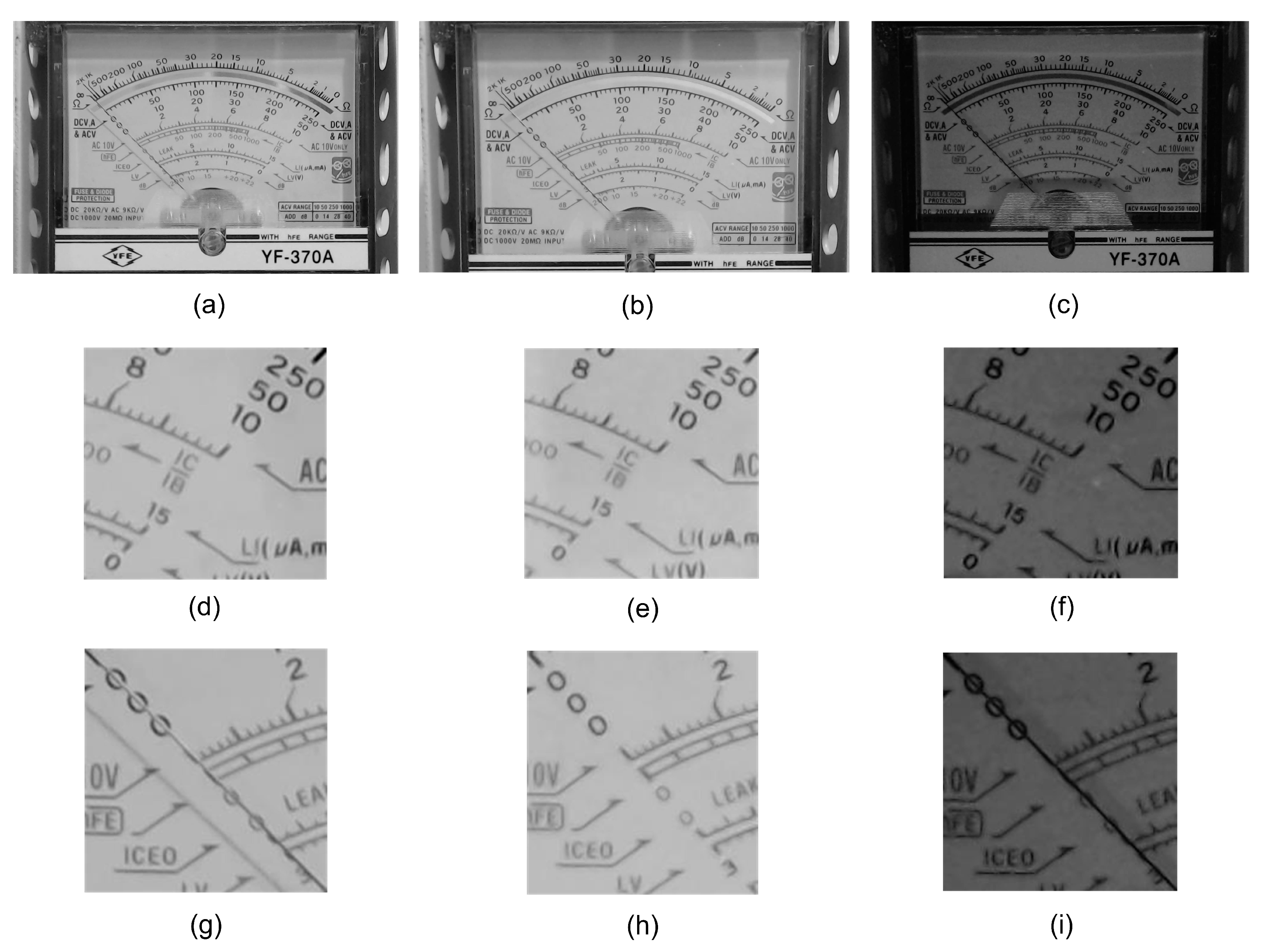
Figure 1.
(a) Illustration of people using the A-meter (model YF-370A) to measure a 1 KΩ resistor. (b) The measured resistor can be identified by the four-band of colors (brown-black-red-gold) which represents (Ω) [2]. Note that (c) the selector arrow of the function selector is switched to the location of and (d) the pointer in the instrument meter indicates around 100 by observing the nonlinear Ω-scale.

Figure 2.
Flowchart of the proposed approach.

Figure 3.
Framework of this study.
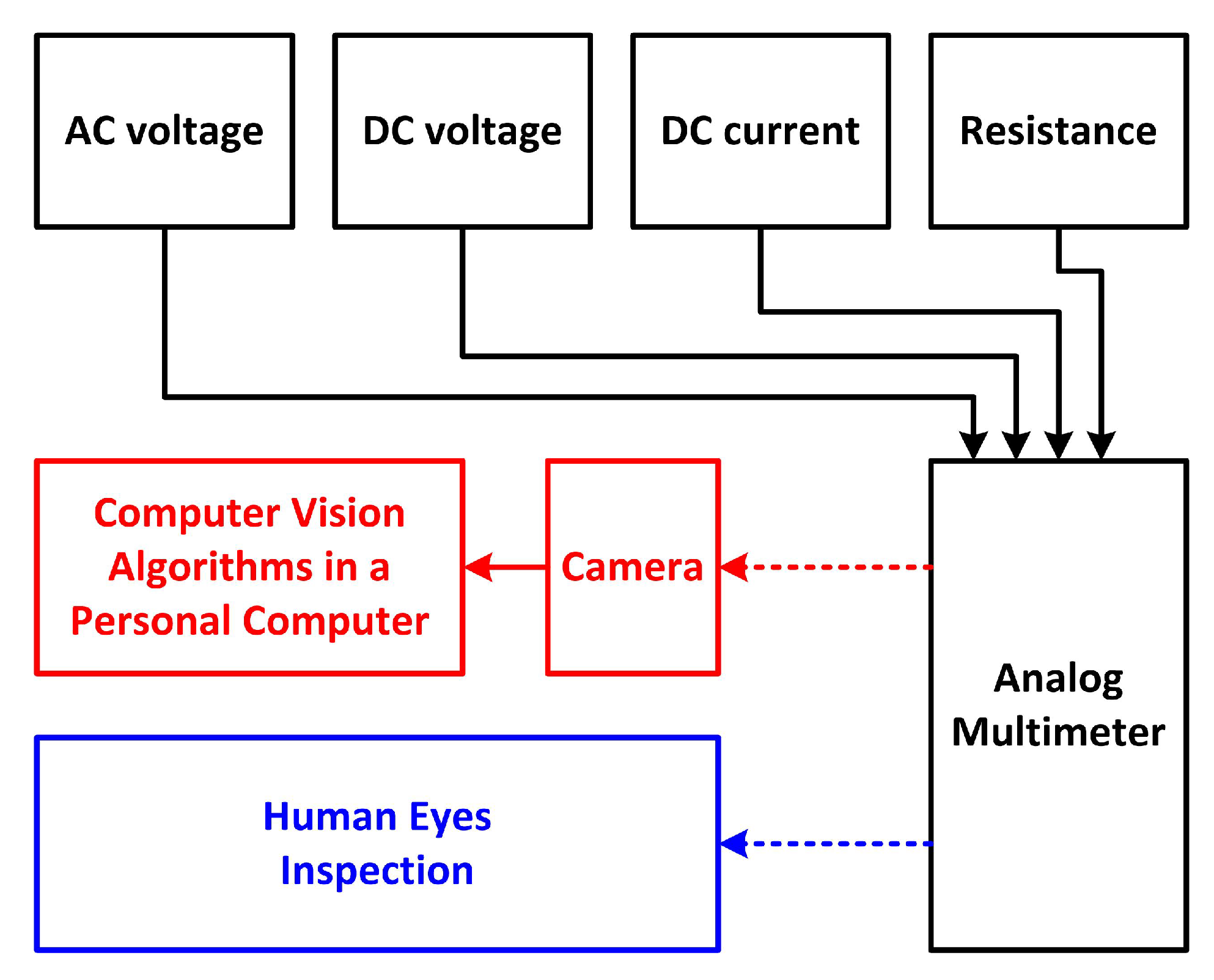
Figure 4.
Experimental devices were set up to develop algorithms and verify the capability of reading an A-meter by computer vision. (a) A standard resistance box (DC resistance controller ZX99A [20]) was used to output resistance to the probe of the A-meter to build lookup data and measure resistance. (b) Measuring the DC current of a 1.5 Vdc battery.

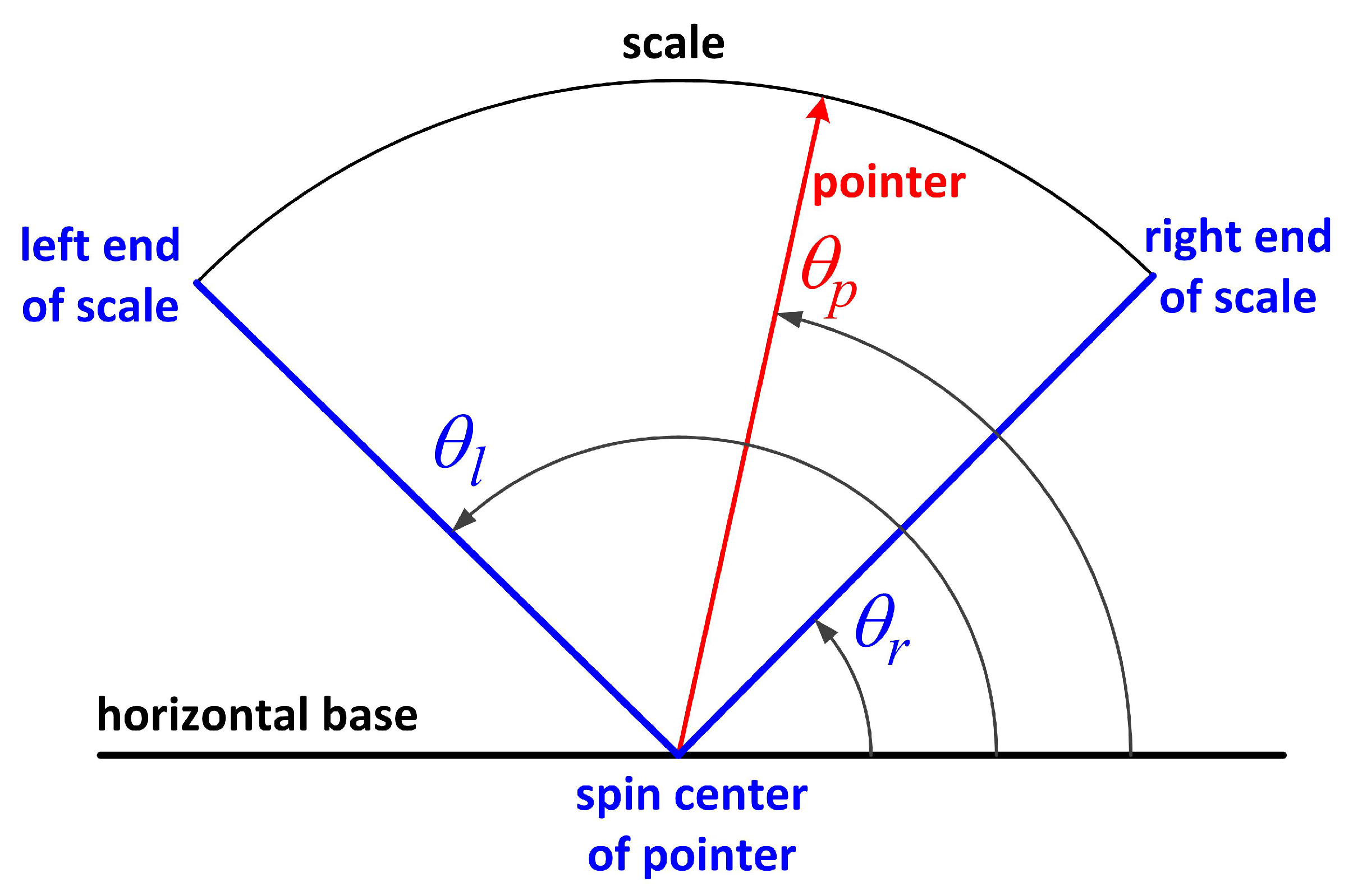
Figure 5.
Relationship between the pointer indicated by and the scale in the of the A-meter where the scale is confined within the range from to .
Figure 5.
Relationship between the pointer indicated by and the scale in the of the A-meter where the scale is confined within the range from to .

Figure 6.
A template () used in the EGM method for the horizontal alignment of the A-meter image.

Figure 7.
(a) The template () used in the EGM method and (b) the bright template () and (c) the dark template () used in the PGM method to locate . (d) The template () used in the EGM method and (e) the bright template () and (f) the dark template () used in the PGM method to locate . (g) The template () used in the EGM method and (h) the bright template () and (i) dark template () used in the PGM method to locate .

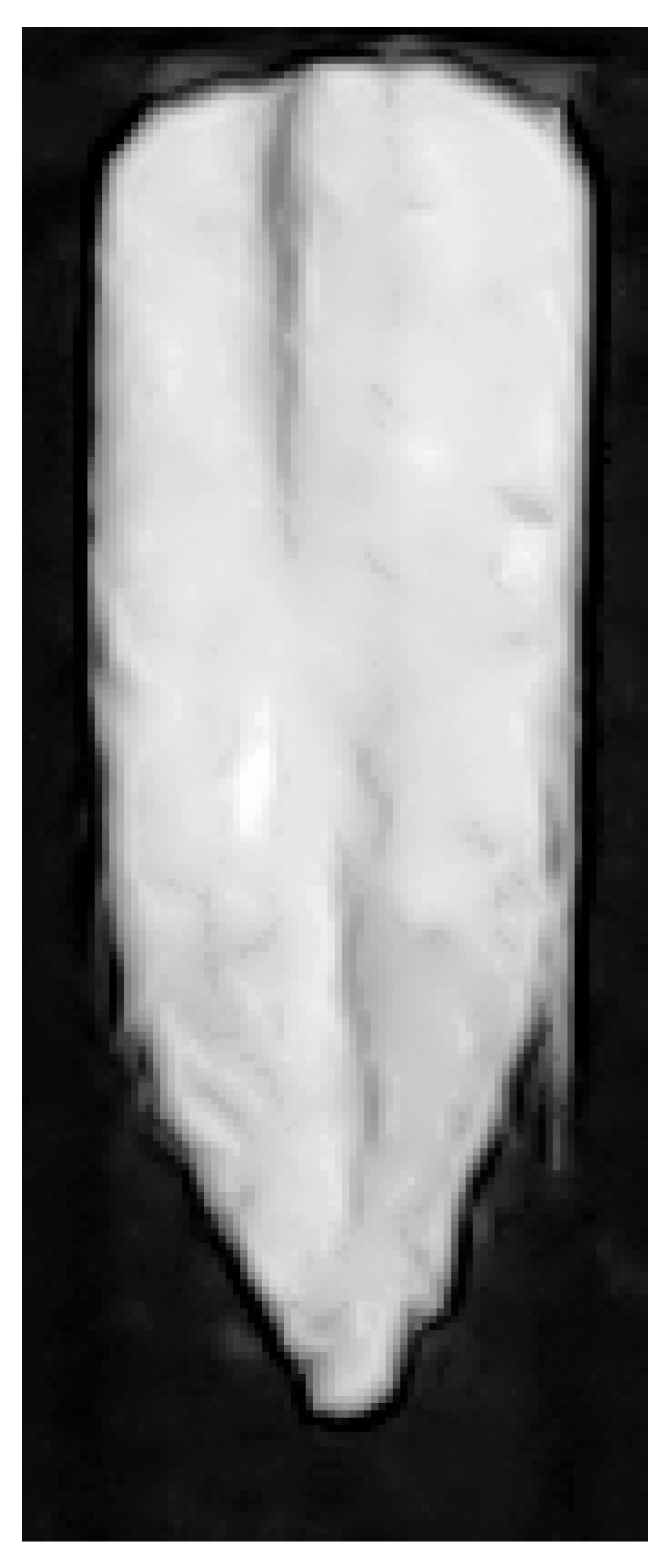
Figure 8.
A template used in the PGM method to detect .

Figure 9.
Relationship between the pointer indicated by and scale in the of the A-meter by adding the coordinates of and those of , where the scale is confined within the range from to . Note here that the straight line of the right-end of scale passes approximately over and and that of left end of scale passes approximately over and , which helps with the calculation of the spin center of pointer . The origin (0, 0) is the top-left coordinate of the image.

Figure 10.
(a–c) illustrate that the templates, , and , given respectively in Figure 7d–f ,were selected with a rectangular ROI so that one pair of diagonal corner points were just passed over by a dummy straight line of the right-end scale; (d–f) illustrate that the templates, , and , given respectively in Figure 7g–i, were selected with a rectangular ROI so that one pair of diagonal corner points were just passed over by a dummy straight line of the left-end scale.

Figure 11.
Illustration of our scanning approach to detect the position of pointer . The scanning direction is from to , i.e., the range (), to find where the corresponding scanline indicates the largest gradient change with zero-crossing property in the profile of .
Figure 11.
Illustration of our scanning approach to detect the position of pointer . The scanning direction is from to , i.e., the range (), to find where the corresponding scanline indicates the largest gradient change with zero-crossing property in the profile of .

Figure 12.
(a) The acquired image () from measuring the 1KΩ resistor by the A-meter YF-370A, where the gray channel of was used for further processing. (b) obtained by Equation (8). (c) Horizontal alignment image () obtained by rotating in (a) minus the . (d) The instrument meter region () detected by means of Equation (12) with the templates given in Figure 7a–c, whereas the selector arrow was detected by Equation (13) with the template given in Figure 8. (e) Within the found , the useful right-end and left-end of the scale were detected by means of Equation (12) with the templates given in Figure 7d–f,g–i, respectively.

Figure 13.
Results obtained by our scanning process. The profiles of (a) , and (b) , were determined by means of the method presented in Section 3.2. According to Equation (20), the detected index was with the corresponding , which is the pointer’s position () in the current illustration.
Figure 13.
Results obtained by our scanning process. The profiles of (a) , and (b) , were determined by means of the method presented in Section 3.2. According to Equation (20), the detected index was with the corresponding , which is the pointer’s position () in the current illustration.
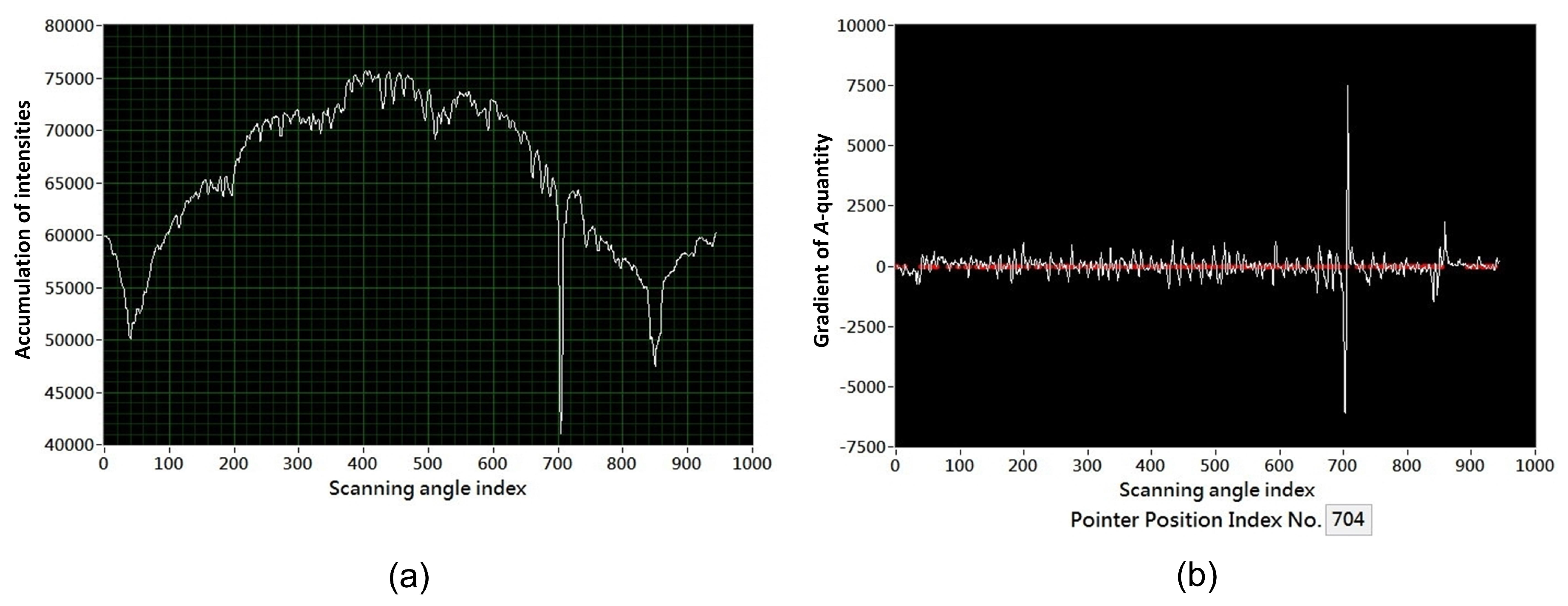
Figure 14.
(a) Low illumination image of the rotated A-meter measuring 110 Vac line power with the function “ACV 250” selected. (b) Its GA-profile. (c) The detection results displayed on the LabVIEW interface that was used to perform our algorithms. Note here that there was a slightly tilted situation in this test. Even the A-meter was rotated 15.947 and the illumination was low with . Tthe result ( Vac) obtained by the proposed method is very close to the Vac observed by the human eye.

Figure 15.
The DC resistance controller ZX99A [20] was used to provide the reference resistance to validate the performance of reading resistance from the A-meter by the proposed method.
Figure 15.
The DC resistance controller ZX99A [20] was used to provide the reference resistance to validate the performance of reading resistance from the A-meter by the proposed method.
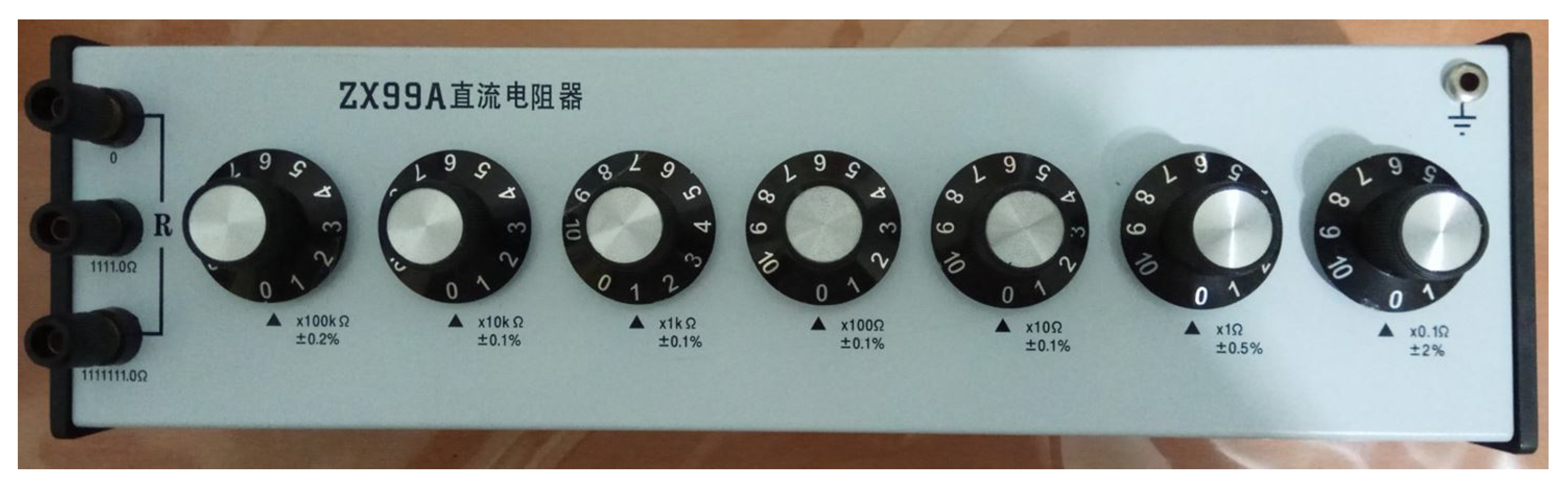
Figure 16.
(a) Rotating the camera left will make the A-meter in the captured image rotate to the right. (b) Rotating the camera right will make the A-meter in the captured image rotate to the left.
Figure 16.
(a) Rotating the camera left will make the A-meter in the captured image rotate to the right. (b) Rotating the camera right will make the A-meter in the captured image rotate to the left.

Figure 17.
An illustrative result directly displayed on the LabVIEW environment for scenario (2), “A-meter rotated right” (24.639), presented in Section 5.3.
Figure 17.
An illustrative result directly displayed on the LabVIEW environment for scenario (2), “A-meter rotated right” (24.639), presented in Section 5.3.

Figure 18.
An illustrative result directly displayed on the LabVIEW environment for scenario (5), “A-meter rotated left” (23.484), presented in Section 5.3.
Figure 18.
An illustrative result directly displayed on the LabVIEW environment for scenario (5), “A-meter rotated left” (23.484), presented in Section 5.3.
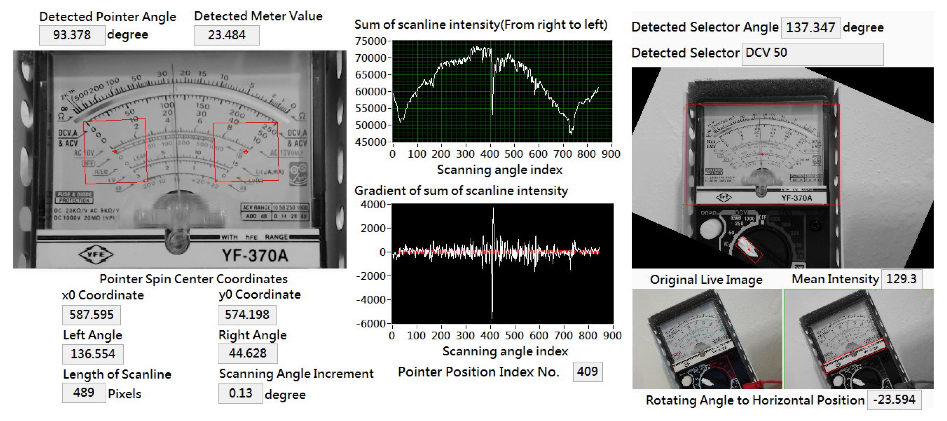
Figure 19.
Plots of the measured DC voltages by our computer vision-based approach for reading the A-meter with different translations and/or rotations. The ground truth was 24 Vdc (the DC voltage), as provided by a tester calibrator (model AOIP CMU 310).
Figure 19.
Plots of the measured DC voltages by our computer vision-based approach for reading the A-meter with different translations and/or rotations. The ground truth was 24 Vdc (the DC voltage), as provided by a tester calibrator (model AOIP CMU 310).

Figure 20.
The effective range to place the camera in to read the A-meter is roughly confined within the zone bounded by the edges among B-C-D-E-F-G-B. If the camera is placed outside this region (e.g., H and I), the reading of the A-meter will fail.
Figure 20.
The effective range to place the camera in to read the A-meter is roughly confined within the zone bounded by the edges among B-C-D-E-F-G-B. If the camera is placed outside this region (e.g., H and I), the reading of the A-meter will fail.

Figure 21.
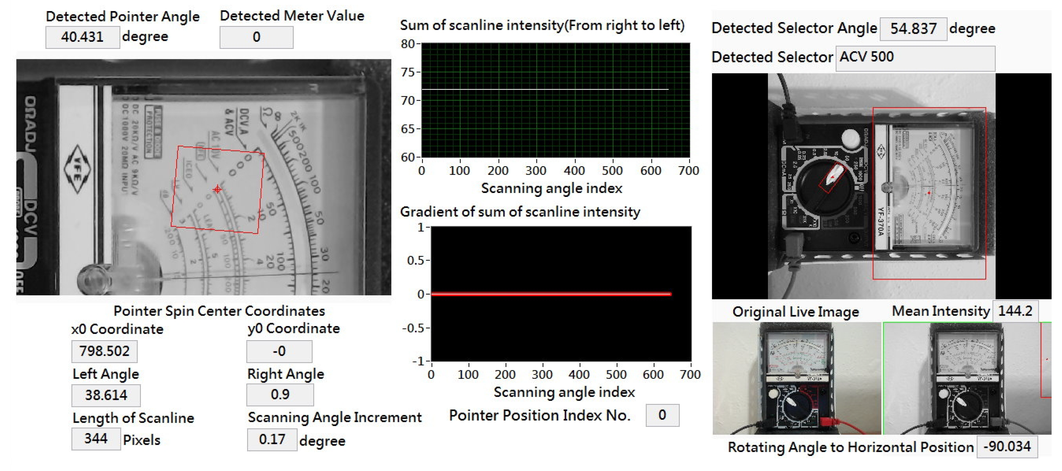
Reading the A-meter fails for the camera placed at H as indicated in Figure 20.
Figure 21.
Reading the A-meter fails for the camera placed at H as indicated in Figure 20.
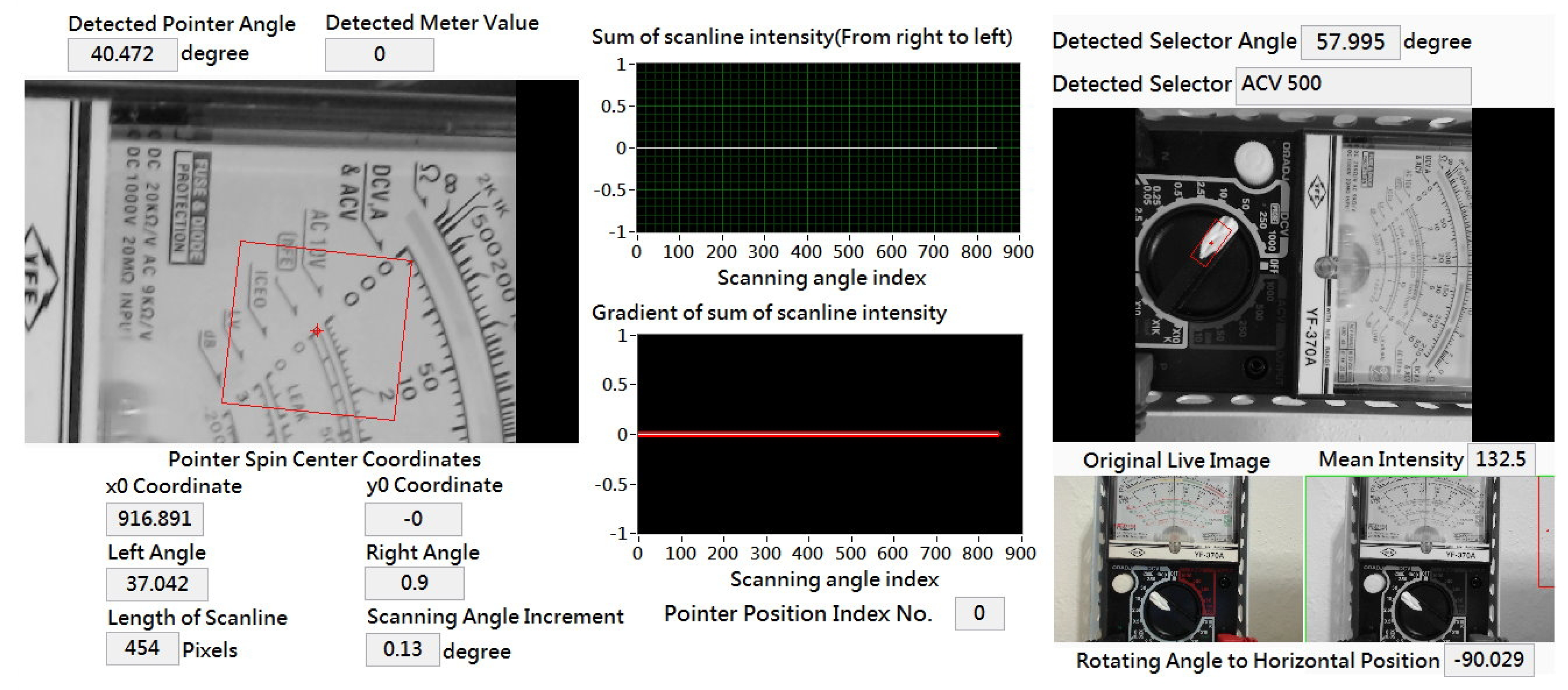
Figure 22.
Reading the A-meter fails for the camera placed at I as indicated in Figure 20.
Figure 22.
Reading the A-meter fails for the camera placed at I as indicated in Figure 20.

Figure 23.
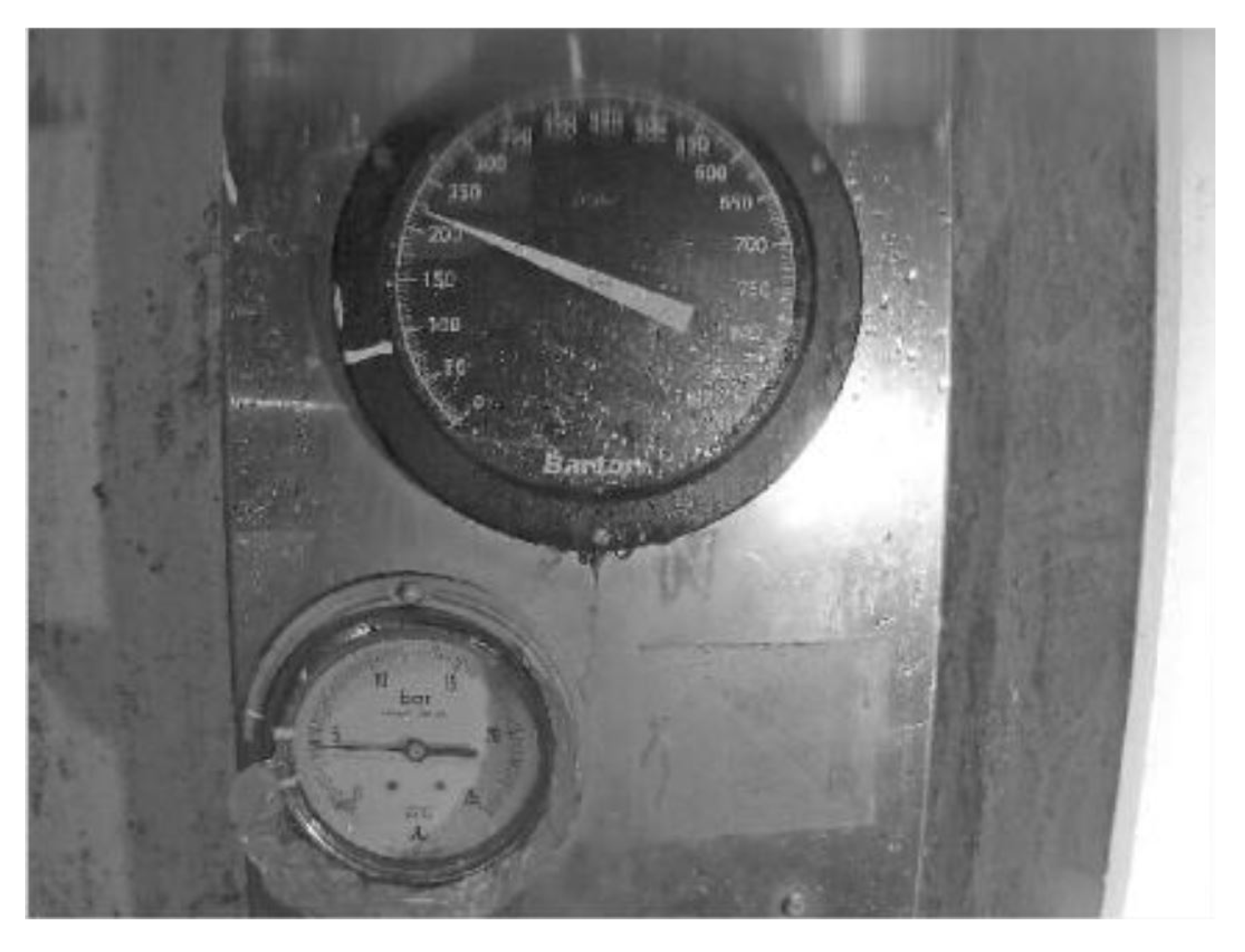
(a) A 15 m Liquid nitrogen (LN2) tank setup at outside our laboratory. (b) The two significant meters installed on the LN2 tank are the level meter (top) and pressure meter (bottom), and an Internet Protocol (IP) camera is used to monitor these two meters. (c) The LN2 tank meters are illuminated by a road lamp and a LED floodlight at night.
Figure 23.
(a) A 15 m Liquid nitrogen (LN2) tank setup at outside our laboratory. (b) The two significant meters installed on the LN2 tank are the level meter (top) and pressure meter (bottom), and an Internet Protocol (IP) camera is used to monitor these two meters. (c) The LN2 tank meters are illuminated by a road lamp and a LED floodlight at night.

Figure 24.
One frame containing the level and pressure meters from a video stream on a rainy night.

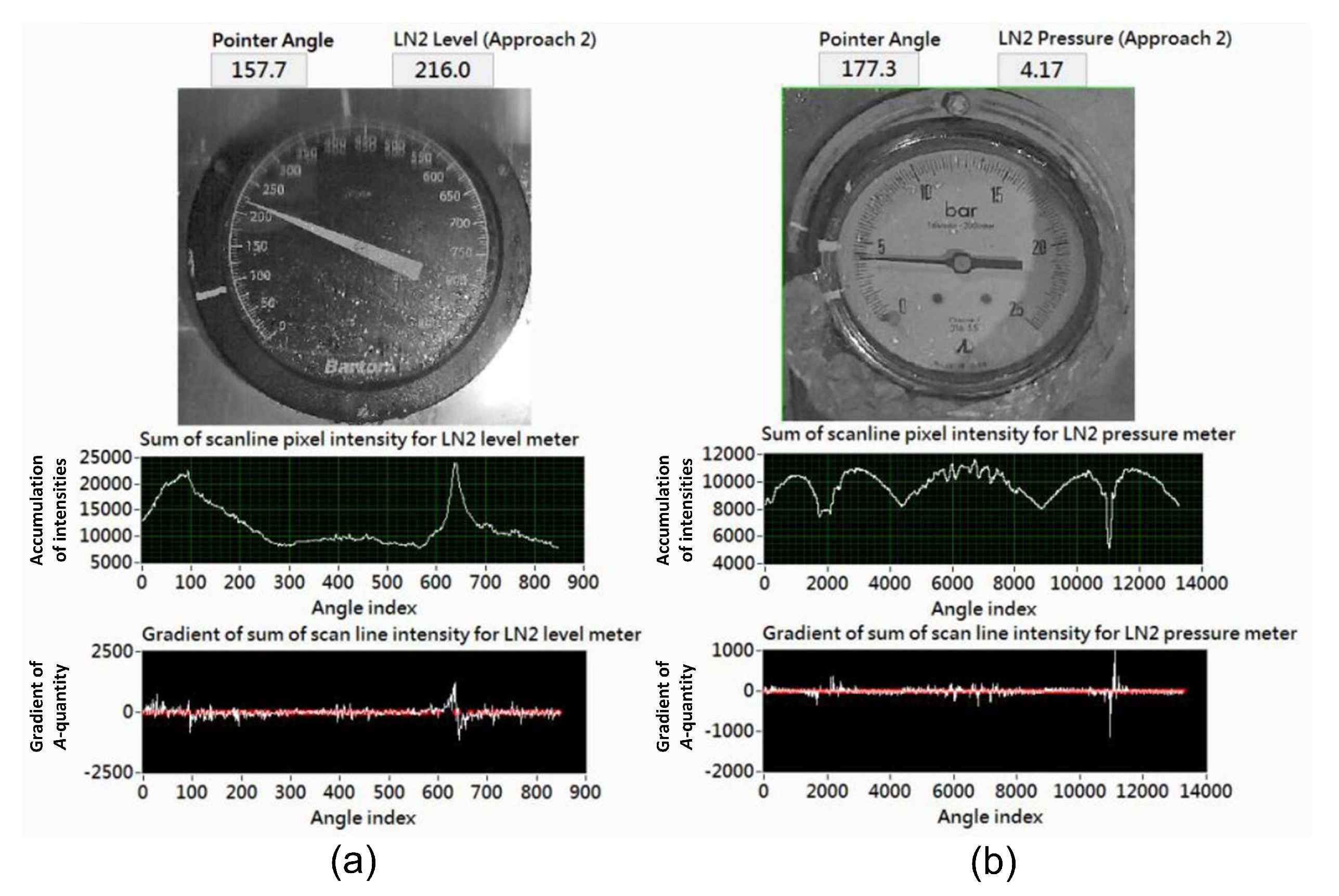
Figure 25.
Results of reading (a) the level meter and (b) the pressure meter the rainy night scenario given in Figure 24.
Figure 25.
Results of reading (a) the level meter and (b) the pressure meter the rainy night scenario given in Figure 24.

Figure 26.
Results of reading (a) the level meter and (b) the pressure meter for the worst-case rainy night scenario.
Figure 26.
Results of reading (a) the level meter and (b) the pressure meter for the worst-case rainy night scenario.


Table 1.
The mapping table for the selector arrow built with the relationship between and , based on Equation (1). Here, and . The auxiliary value, , represents the maximum value used in linear cases (i.e., ) and the multiplier used in nonlinear cases (i.e., ), respectively. Here “NA” denotes “not available.”
| Index of Function, | Auxiliary Value, | Function Name | Orientation Range |
|---|---|---|---|
| 0 | 10 | ACV 10 | |
| 1 | 50 | ACV 50 | |
| 2 | 250 | ACV 250 | |
| 3 | 500 | ACV 500 | |
| 4 | 1000 | ACV 1000 | |
| 5 | NA | OFF | |
| 6 | 1000 | DCV 1000 | |
| 7 | 250 | DCV 250 | |
| 8 | 50 | DCV 50 | |
| 9 | 10 | DCV 10 | |
| 10 | 2.5 | DCV 2.5 | |
| 11 | 0.5 | DCV 0.5 | |
| 12 | 0.25/0.05 | DCV 0.25/DCmA 0.05 | |
| 13 | 2.5 | DCmA 2.5 | |
| 14 | 25 | DCmA 25 | |
| 15 | 250 | DCmA 250 | |
| 16 | 1 | ||
| 17 | 10 | ||
| 18 | 1000 | K | |
| 19 | 10000 | K |
Table 2.
Nonlinear mapping table built for measuring the resistance from the pointer indication on the Ω-scale where the ground-truth angle corresponded to the resistance value which was obtained by means of a protractor. The values listed here were used in the current study.
Table 2.
Nonlinear mapping table built for measuring the resistance from the pointer indication on the Ω-scale where the ground-truth angle corresponded to the resistance value which was obtained by means of a protractor. The values listed here were used in the current study.
| Index, k | Resistance Value, | Ground-Truth Angle, |
|---|---|---|
| 0 | 0 | |
| 1 | 1 | |
| 2 | 2 | |
| 3 | 2.5 | |
| 4 | 3 | |
| 5 | 4 | |
| 6 | 4.5 | |
| 7 | 5 | |
| 8 | 5.4 | |
| 9 | 5.6 | |
| 10 | 7 | |
| 11 | 7.2 | |
| 12 | 7.4 | |
| 13 | 9 | |
| 14 | 10 | |
| 15 | 11 | |
| 16 | 12 | |
| 17 | 13 | |
| 18 | 14 | |
| 19 | 15 | |
| 20 | 16 | |
| 21 | 17 | |
| 22 | 18 | |
| 23 | 19 | |
| 24 | 20 | |
| 25 | 22 | |
| 26 | 24 | |
| 27 | 26 | |
| 28 | 28 | |
| 29 | 30 | |
| 30 | 32 | |
| 31 | 34 | |
| 32 | 36 | |
| 33 | 38 | |
| 34 | 40 | |
| 35 | 42 | |
| 36 | 44 | |
| 37 | 46 | |
| 38 | 48 | |
| 39 | 50 | |
| 40 | 55 | |
| 41 | 60 | |
| 42 | 65 | |
| 43 | 70 | |
| 44 | 75 | |
| 45 | 80 | |
| 46 | 90 | |
| 47 | 100 | |
| 48 | 120 | |
| 49 | 140 | |
| 50 | 180 | |
| 51 | 200 | |
| 52 | 300 | |
| 53 | 400 | |
| 54 | 500 | |
| 55 | 1000 | |
| 56 | 2000 | |
| 57 | ∞ |
| Located R | Input Image I | Template for EGM | Bright Template for PGM | Dark Template for PGM |
|---|---|---|---|---|
| in Figure 7a | in Figure 7b | in Figure 7c | ||
| in Figure 7d | in Figure 7e | in Figure 7f | ||
| in Figure 7g | in Figure 7h | in Figure 7i |
Table 4.
Results of using the A-meter YF-370A with the function select “OFF”.
| Accuracy (%) | ||||||
|---|---|---|---|---|---|---|
| 0.129 | 138.5 | OFF | 0 | OFF | 0 | 100% |
| 18.314 | 31.9 | OFF | 0 | OFF | 0 | 100% |
| 32.324 | 76.0 | OFF | 0 | OFF | 0 | 100% |
| −16.257 | 37.9 | OFF | 0 | OFF | 0 | 100% |
| −21.814 | 140.6 | OFF | 0 | OFF | 0 | 100% |
Table 5.
Results of using A-meter YF-370A with function select “ACV 250” to measure the 110Vac line power. The mean accuracy was 97.28%.
Table 5.
Results of using A-meter YF-370A with function select “ACV 250” to measure the 110Vac line power. The mean accuracy was 97.28%.
| (Vac) | (Vac) | Accuracy (%) | ||||
|---|---|---|---|---|---|---|
| 0 | 122.2 | ACV 250 | 106 | ACV 250 | 110.370 | 96.19% |
| * 15.947 | 49.8 | ACV 250 | 108 | ACV 250 | 107.444 | 99.49% |
| 15.967 | 74.9 | ACV 250 | 106 | ACV 250 | 111.511 | 94.80% |
| −15.117 | 128.4 | ACV 250 | 108 | ACV 250 | 109.959 | 98.19% |
| −18.969 | 15.6 | ACV 250 | 112.5 | ACV 250 | 115.077 | 97.71% |
* Slightly tilted surface.
Table 6.
Results of using A-meter YF-370A with function select “ACV 250” to measure the 220 Vac line power. The mean accuracy was 98.86%, where the accuracy of the fifth data point is not available since it was difficult to read with the human eye under very low illumination ().
Table 6.
Results of using A-meter YF-370A with function select “ACV 250” to measure the 220 Vac line power. The mean accuracy was 98.86%, where the accuracy of the fifth data point is not available since it was difficult to read with the human eye under very low illumination ().
| (Vac) | (Vac) | Accuracy (%) | ||||
|---|---|---|---|---|---|---|
| −1.245 | 124.7 | ACV 250 | 225 | ACV 250 | 229.775 | 97.88% |
| 11.303 | 55.6 | ACV 250 | 225 | ACV 250 | 225.682 | 99.70% |
| 29.985 | 73.2 | ACV 250 | 224 | ACV 250 | 223.604 | 99.82% |
| −17.144 | 61.5 | ACV 250 | 225 | ACV 250 | 229.434 | 98.03% |
| −21.066 | 7.5 | Difficult to read | ACV 250 | 236.450 | NA | |
Table 7.
Results from using the A-meter YF-370A with function select (a) “DCV 2.5” to measure the 1.5 Vdc battery, (b) “DCV 10” to measure the 5 Vdc adaptor, (c) “DCV 10” to measure the 7.5 Vdc adaptor, (d) “DCV 10” to measure the 9 Vdc battery, (e) “DCV 50” to measure the 12 Vdc adaptor, (f) “DCV 50” to measure the 24 Vdc adaptor, and (g) “DCmA 25” to measure the DC current of the 1.5 V battery.
| (a) Mean accuracy = 96.26% | ||||||
| (Vdc) | (Vdc) | Accuracy(%) | ||||
| 0 | 124.4 | DCV 2.5 | 1.3 | DCV 2.5 | 1.331 | 97.62% |
| 13.776 | 46.9 | DCV 2.5 | 1.3 | DCV 2.5 | 1.343 | 96.69% |
| * 22.618 | 140.4 | DCV 2.5 | 1.225 | DCV 2.5 | 1.328 | 91.59% |
| −16.801 | 128.6 | DCV 2.5 | 1.35 | DCV 2.5 | 1.379 | 97.85% |
| −12.559 | 34.7 | DCV 2.5 | 1.26 | DCV 2.5 | 1.291 | 97.54% |
| (b) Mean accuracy = 95.15% | ||||||
| (Vdc) | (Vdc) | Accuracy(%) | ||||
| −0.045 | 134.9 | DCV 10 | 5.1 | DCV 10 | 4.757 | 93.27% |
| 14.166 | 128.4 | DCV 10 | 5 | DCV 10 | 4.657 | 93.14% |
| 28.847 | 38.4 | DCV 10 | 4.81 | DCV 10 | 5.162 | 92.68% |
| −14.337 | 105.2 | DCV 10 | 5.1 | DCV 10 | 5.084 | 99.69% |
| −29.657 | 41.3 | DCV 10 | 5 | DCV 10 | 5.152 | 96.96% |
| (c) Mean accuracy = 97.06% | ||||||
| (Vdc) | (Vdc) | Accuracy(%) | ||||
| 1.328 | 95.3 | DCV 10 | 7.7 | DCV 10 | 7.519 | 97.65% |
| 25.032 | 37.7 | DCV 10 | 7.2 | DCV 10 | 7.177 | 99.68% |
| 16.194 | 126.8 | DCV 10 | 7.9 | DCV 10 | 7.212 | 91.29% |
| −16.977 | 132.8 | DCV 10 | 7.5 | DCV 10 | 7.403 | 98.71% |
| −31.175 | 52.5 | DCV 10 | 7.41 | DCV 10 | 7.561 | 97.96% |
| (d) Mean accuracy = 99.27% | ||||||
| (Vdc) | (Vdc) | Accuracy(%) | ||||
| 1.55 | 132.7 | DCV 10 | 9.1 | DCV 10 | 9.027 | 99.20% |
| 24.932 | 42.9 | DCV 10 | 8.59 | DCV 10 | 8.572 | 99.79% |
| −19.011 | 68.1 | DCV 10 | 8.7 | DCV 10 | 8.769 | 99.21% |
| 28.253 | 127.1 | DCV 10 | 8.9 | DCV 10 | 8.986 | 99.03% |
| −4.976 | 33.7 | DCV 10 | 8.69 | DCV 10 | 8.768 | 99.10% |
| (e) Mean accuracy = 94.66% | ||||||
| (Vdc) | (Vdc) | Accuracy(%) | ||||
| 0.639 | 133.6 | DCV 50 | 11 | DCV 50 | 11.845 | 92.32% |
| 15.813 | 46.6 | DCV 50 | 11.4 | DCV 50 | 12.103 | 93.83% |
| 17.861 | 74.9 | DCV 50 | 11 | DCV 50 | 11.159 | 98.55% |
| −12.345 | 35.6 | DCV 50 | 11 | DCV 50 | 11.668 | 93.93% |
| −14.098 | 7.2 | Difficult to read | DCV 50 | 12.385 | NA | |
| (f) Mean accuracy = 94.72% | ||||||
| (Vdc) | (Vdc) | Accuracy(%) | ||||
| 0 | 52.1 | DCV 50 | 23 | DCV 50 | 24.695 | 92.63% |
| 28.829 | 74.8 | DCV 50 | 23 | DCV 50 | 22.073 | 95.97% |
| −0.055 | 67.7 | DCV 50 | 22.9 | DCV 50 | 23.836 | 95.91% |
| −29.672 | 44.2 | DCV 50 | 23 | DCV 50 | 24.574 | 93.16% |
| −14.997 | 16.8 | DCV 50 | 23 | DCV 50 | 24.025 | 95.94% |
| (g) Mean accuracy = 96.85% | ||||||
| (Vdc) | (Vdc) | Accuracy(%) | ||||
| −0.757 | 40.3 | DCmA 25 | 10.3 | DCmA 25 | 10.391 | 99.12% |
| 22.184 | 39.8 | DCmA 25 | 9.5 | DCmA 25 | 9.639 | 98.54% |
| * 13.007 | 54.7 | DCmA 25 | 10.2 | DCmA 25 | 10.425 | 97.79% |
| −30.043 | 134.9 | DCmA 25 | 11 | DCmA 25 | 11.311 | 97.17% |
| −16.447 | 133.7 | DCmA 25 | 11 | DCmA 25 | 10.080 | 91.64% |
* Tilted surface.
Table 8.
Results of using the A-meter YF-370A with function select (a) “” to measure the resistance of the 50 Ω resistor, (b) “” to measure the resistance of the 220 Ω resistor, (c) “” to measure the resistance of the 1 KΩ resistor, (d) “K” to measure the resistance of the 1 KΩ resistor, and (e) “ K” to measure the resistance of the 70 KΩ resistor.
| (a) Mean accuracy = 97.26% | ||||||
| (Ω) | (Ω) | Accuracy(%) | ||||
| −0.04 | 140.5 | 54 | 53.89 | 99.80% | ||
| 24.185 | 74.4 | 55 | 54.39 | 98.89% | ||
| 20 | 123.5 | 55 | 56.47 | 97.33% | ||
| −21.884 | 16.2 | 51 | 50.65 | 99.31% | ||
| −20.187 | 12.4 | 55 | 50.04 | 90.98% | ||
| (b) Mean accuracy = 97.52% | ||||||
| (Ω) | (Ω) | Accuracy(%) | ||||
| 0.063 | 74.9 | 240 | 229.6 | 95.67% | ||
| 9.82 | 133.6 | 238 | 228.6 | 96.05% | ||
| 15.538 | 54.1 | 240 | 239.7 | 99.88% | ||
| −23.738 | 60.2 | 232 | 233 | 99.57% | ||
| −15.028 | 40.7 | 228 | 219.9 | 96.45% | ||
| (c) Mean accuracy = 99.58% | ||||||
| (Ω) | (Ω) | Accuracy(%) | ||||
| 16.935 | 131.4 | 1000 | 999.8 | 99.98% | ||
| −17.859 | 131.6 | 1000 | 1004 | 99.60% | ||
| −14.622 | 65 | 1000 | 1004 | 99.60% | ||
| 25.365 | 76.4 | 1000 | 1009 | 99.10% | ||
| 23.235 | 17.8 | 1000 | 1004 | 99.60% | ||
| (d) Mean accuracy = 87.27% | ||||||
| (Ω) | (Ω) | Accuracy(%) | ||||
| * −1.052 | 74.8 | K | 1000 | K | 1089 | 91.10% |
| −15 | 11.6 | K | 990 | K | 1188 | 80.00% |
| −25.006 | 71.7 | K | 1000 | K | 1132 | 86.80% |
| 19.758 | 134.7 | K | 1000 | K | 1176 | 82.40% |
| 10.793 | 63.4 | K | 990 | K | 950.8 | 96.04% |
| (e) Mean accuracy = 99.42% | ||||||
| (Ω) | (Ω) | Accuracy(%) | ||||
| 0.577 | 62.1 | K | 71000 | K | 70090 | 98.72% |
| 5.971 | 8.6 | K | 72000 | K | 72050 | 99.93% |
| 14.766 | 139.5 | K | 70000 | K | 70100 | 99.85% |
| −12.13 | 93.5 | K | 70000 | K | 69070 | 98.67% |
| −15.066 | 22.2 | K | 70000 | K | 69950 | 99.93% |
* Tilted surface.
Table 9.
Results of reading the A-meter YF-370A with 15.425 rotation for the measurement of the 110 Vac line power under variant illumination.
Table 9.
Results of reading the A-meter YF-370A with 15.425 rotation for the measurement of the 110 Vac line power under variant illumination.
| (Vac) | (Vac) | Accuracy (%) | |
|---|---|---|---|
| 133.6 | 109 | 111.039 | 98.14% |
| 129.5 | 110 | 113.439 | 96.87% |
| 123.1 | 109 | 111.419 | 97.78% |
| 95.3 | 109 | 110.226 | 98.88% |
| 54.0 | 107.5 | 111.742 | 96.05% |
| 48.3 | 109.5 | 113.448 | 96.39% |
| 40.7 | 108 | 112.083 | 96.22% |
| 36.7 | 110 | 112.111 | 98.08% |
| 23.0 | 107.5 | 112.083 | 95.74% |
| 8.1 | 110 | 114.130 | 96.25% |
| 7.5 | Difficult to read | 113.107 | NA |
| 6.0 | Difficult to read | Fail to locate | NA |
| 5.8 | Difficult to read | Fail to locate | NA |
Table 10.
Results of comparing the measurements () with a digital multimeter (model DMM-85) to those () with the A-meter YF-370A read by the proposed method. The mean accuracy was 95.61%.
Table 10.
Results of comparing the measurements () with a digital multimeter (model DMM-85) to those () with the A-meter YF-370A read by the proposed method. The mean accuracy was 95.61%.
| Measurement Target | Accuracy (%) | |||||
|---|---|---|---|---|---|---|
| 12 | 31.7 | 5 Vdc adaptor | 5.36 Vdc | DCV 10 | 5.239 Vdc | 97.74% |
| −25 | 16.6 | 7.5 Vdc adaptor | 8.06 Vdc | DCV 10 | 7.676 Vdc | 95.24% |
| 18 | 128 | 110 Vac line power | 113.6 Vac | ACV 250 | 113.244 Vac | 99.69% |
| 19 | 127.3 | 220 Vac line power | 227 Vac | ACV 250 | 227.56 Vac | 99.75% |
| 0 | 67.7 | DC current * | 7.53 mA | DCmA 25 | 6.943 mA | 92.20% |
| 9 | 126.8 | 470 Ω | 469 Ω | 488.4 Ω | 95.86% | |
| −17 | 74.8 | 10 KΩ | 9.97 KΩ | K | 11.09 KΩ | 88.77% |
* 1.5Vdc battery; Resistance provided by the DC resistance controller ZX99A [20].
Table 11.
Statistical results of the measured DC voltages plotted in Figure 19.
Table 11.
Statistical results of the measured DC voltages plotted in Figure 19.
| Scenario | Mean Measured Value (Vdc) | Mean Accuracy (%) |
|---|---|---|
| (1) Shifted right | 24.388 | 98.38% |
| (2) Rotated right | 24.260 | 98.80% |
| (3) Shifted right and rotated left | 24.432 | 98.19% |
| (4) Shifted left | 23.538 | 97.97% |
| (5) Rotated left | 23.455 | 97.73% |
| (6) Shifted left and rotated right | 23.719 | 98.83% |
Table 12.
Statistical results for the camera located at B, C, D, E, F, and G of the effective range drawn in Figure 20.
Table 12.
Statistical results for the camera located at B, C, D, E, F, and G of the effective range drawn in Figure 20.
| Camera Location | Mean Measured Value (Vdc) | Mean Accuracy (%) |
|---|---|---|
| B | 23.960 | 99.14% |
| C | 23.811 | 98.98% |
| D | 23.807 | 99.09% |
| E | 23.598 | 95.81% |
| F | 23.706 | 98.32% |
| G | 23.447 | 97.19% |
© 2018 by the authors. Licensee MDPI, Basel, Switzerland. This article is an open access article distributed under the terms and conditions of the Creative Commons Attribution (CC BY) license (http://creativecommons.org/licenses/by/4.0/).
Share and Cite
MDPI and ACS Style
Chen, Y.-S.; Wang, J.-Y. Computer Vision-Based Approach for Reading Analog Multimeter. Appl. Sci. 2018, 8, 1268. https://doi.org/10.3390/app8081268
AMA Style
Chen Y-S, Wang J-Y. Computer Vision-Based Approach for Reading Analog Multimeter. Applied Sciences. 2018; 8(8):1268. https://doi.org/10.3390/app8081268
Chicago/Turabian StyleChen, Yung-Sheng, and Jeng-Yau Wang. 2018. "Computer Vision-Based Approach for Reading Analog Multimeter" Applied Sciences 8, no. 8: 1268. https://doi.org/10.3390/app8081268
Note that from the first issue of 2016, this journal uses article numbers instead of page numbers. See further details here.