Multiellipsoidal Mapping Algorithm

Abstract

The robotic mapping problem, which consists in providing a spatial model of the environment to a robot, is a research topic with a wide range of applications. One important challenge of this problem is to obtain a map that is information-rich (i.e., a map that preserves main structures of the environment and object shapes) yet still has a low memory cost. Point clouds offer a highly descriptive and information-rich environmental representation; accordingly, many algorithms have been developed to approximate point clouds and lower the memory cost. In recent years, approaches using basic and “simple” (i.e., using only planes or spheres) geometric entities for approximating point clouds have been shown to provide accurate representations at low memory cost. However, a better approximation can be implemented if more complex geometric entities are used. In the present paper, a new object-mapping algorithm is introduced for approximating point clouds with multiple ellipsoids and other quadratic surfaces. We show that this algorithm creates maps that are rich in information yet low in memory cost and have features suitable for other robotics problems such as navigation and pose estimation.

1. Introduction

Many algorithms have been developed for the robotic mapping problem [1], which arises when a robot is provided with a spatial model of the environment. Unlike many 3D reconstruction algorithms that use interpolation to obtain the best object rendering, the principal aim of robotic mapping is to create maps that are rich in information and low in memory cost. The environment and objects could be acquired through 3D sensor like Laser Rangefinder or multiples camera view with algorithms like Structure from Motion [2]. With these techniques we obtain dense point clouds.

On the one hand, there exist 3D mapping algorithms, e.g., Simultaneous Localization and Mapping (SLAM), that model key point maps. The principal features of such algorithms are representations with low memory cost and ease of use. However, the maps are not information-rich; consequently, such algorithms cannot be used in many applications, such as object manipulation and aerial navigation. On the other hand, many algorithms create extensive object representations as 3D reconstructions based on the Radial Basis Function (RBF) [3] or other functions [4], resulting in richer information maps, albeit at a high memory cost; additionally, such algorithms are difficult to use. Finding a good balance between representation and memory cost is an important current research topic.

In the last decade, algorithms based on object mapping with geometric entities have become very popular for many applications [1], such as urban and office environment mapping. Object mapping refers to algorithms that approximate the volume shape of a point cloud (it is to say approximate a point cloud) with multiply geometric entities, this is analogous to use curve fitting in a regression problem, but we use geometric entities to describe and preserve the volume shapes instead of functions because there is not dependent variables. The quality of the approximation could be measured using the mean distance of the points to the geometric entity.

Geometric entities have been used before to approximate point clouds, for instance, we observe the use of multiplanar representations [5] and spherical and linear representations [6,7,8,9]. Each of these approaches fits the parameters of their geometric entities to obtain the best approximation of sensor data. However, if more complex entities are used, we can obtain approximations of point clouds with better accuracy, and using fewer entities than those obtained by using muliltiplanar, spherical or linear representations.

In this paper, a new object-mapping algorithm is presented. This algorithm is capable of approximating the point cloud with multiple ellipsoids and other quadratic surfaces such as spheres, pairs of planes, and pseudocylinders, which allows us to reduce the number of geometric entities used to represent the objects and complete scenes of the environment, this feature is shown in a controlled experiment, but to automate this process a hierarchical clustering must be implemented, as discussed in the future work section.

This algorithm can also be related to Hyperellipsoidal Neurons (HNs) [10] based on Geometric Algebra (GA) [11], where every neuron is trained with k-means++ [12] and Differential Evolution (DE) [13] for adapting the point cloud implicit surface.

In the following sections, we show that the multiellipsoidal mapping algorithm is capable of creating information-rich maps with low memory cost and that the entities obtained with the algorithm are even capable of deforming into other quadratic surfaces due to their representation in GA as multivectors. The entities are described in GA; then, the map is suitable for developing new algorithms that work in this algebra, such as path planning [14], pose estimation [15,16], and other tasks [17].

The paper is organized as follows. In Section 2, we introduce several mathematical and algorithmic tools used in this paper. Section 3 presents the adaptation strategy of the ellipsoidal surfaces to a point cloud. In Section 4, we explore various experiments to show the performance of the algorithm. In Section 5, the differences from object-mapping algorithms based on function approximations are discussed. Finally, conclusions are presented in Section 6, and in Section 7 we discuss the future work.

2. Mathematical Background

In this section, we introduce the mathematical framework of GA to represent the geometric entities. We also introduce the basic notions of k-means++ and DE algorithms to optimize the representation. The notation shown here will be used in the development of the proposed algorithm.

2.1. Geometric Algebra

GAs are Clifford Algebras [11,18] constructed over a bilinear form of the vector space ${\mathbb{R}}^{p,q,r}$, where $(p,q,r)$ is the algebraic signature. This GA is denoted by ${\mathbb{G}}_{p,q,r}$ and it is an equivalent notation for $C{\ell }_{p,q,r}\left(\mathbb{R}\right)$. The elements that belong to this algebra are called multivectors. Let us denote by “∘” the Clifford product, by “•” the inner product and by “∧” the outer product. Then, for two basis vectors, (1) states the Clifford product behavior, where $e_i\wedge e_j$ is a bivector or a 2-vector element; all vectors in ${\mathbb{R}}^{p,q,r}$ are included in ${\mathbb{G}}_{p,q,r}$ as 1-vectors (a k-vector describe a multivector span by k basis vectors). In addition, the properties of the bilinear form shown in (2) are present, where “·” is the common dot product used in linear algebra, thus ${\mathbb{R}}^{p,q,r}\subset {\mathbb{G}}_{p,q,r}$.

$$e_i\circ e_j=\left\{\begin{array}{cc}{e}_i\wedge e_j& \mathrm{if}i\ne j\hfill \\ 1& \mathrm{if}1\le i=j\le p\hfill \\ -1& \mathrm{if}p<i=j\le q\hfill \\ 0& \mathrm{if}q<i=j\le r\hfill \end{array}\right.$$

(1)

$$a\circ a=a•a=a·a,a\in {\mathbb{R}}^{p,q,r}$$

(2)

GAs are associative and anticommutative algebras; additionally, due to the generality of the Clifford product, many properties of other mathematical frameworks are present [11] such as complex numbers, quaternions, and other Cayley-Dickson algebras, in addition to Pauli matrices and spinor algebras.

Nevertheless, GAs are not only useful for integrating multiple mathematical frameworks but also present attractive features for geometric entity representation. In a GA, multivectors by themselves could represent geometric entities in their inner or outer product representation instead of the traditional geometric locus. The importance of this feature is that the geometric entities, as well as their operators, are represented as elements of the same algebra (both are represented as multivectors).

2.2. Hyperconformal Geometric Algebra

The most used GA is perhaps the Conformal Geometric Algebra (CGA) for the 3D case ${\mathbb{G}}_{4,1}$, where the algebraic signature is $(4,1,0)$, and its extension to n-dimensions ${\mathbb{G}}_{n+1,1}$ to represent the ${\mathbb{R}}^n$ vector space. In this algebra, it is possible to represent points, pairs of points, lines, planes, circles and spheres. Many algorithms for robotics and machine vision [19], e.g., finding path planning algorithms [14], pose estimation [15], structure extraction from motion [16], geometric entity detection [6,7], and robotic mapping algorithms [8,9], have been developed with this algebra.

However, to use more complex geometric entities as algebra elements, other algebras must be used. The GA ${\mathbb{G}}_{6,3}$ [20] is a generalization of ${\mathbb{G}}_{4,1}$, in which such geometric entities like ellipsoids, planes, pair of planes, pseudocylinders, spheres and others deformed quadratic surfaces can be represented as multivectors. In [10], ${\mathbb{G}}_{6,3}$ was extended to any dimension in the so-called Hyperconformal GA (HGA) with a notation ${\mathbb{G}}_{2n,n}$ for representing the vector space ${\mathbb{R}}^n$. 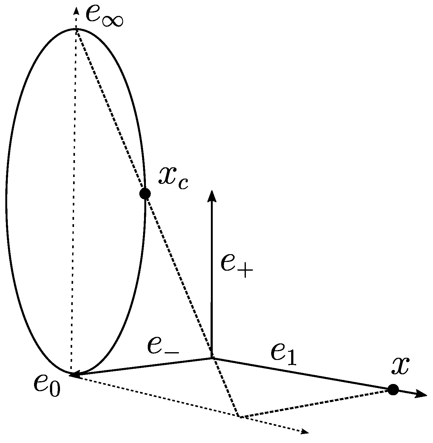This algebra is constructed by using a homogeneous stereographic projection in (3) over every coordinate. Figure 1 describes a graphical representation of the projection.

The null basis are related to (3) by $e_0=e_{+}+e_{-}$ and $e_{\infty }=e_{+}-e_{-}$ and they have the property $e_0^2=e_{\infty }^2=0$. Given a three-dimensional space with basis $(e_x,e_y,e_z)$, the previous notation must be extended. Consider that the stereographic projection is applied in every axis, e.g., the null basis of the coordinate $e_x$ are denoted with $e_{0x}$ and $e_{\infty x}$.

$$x_c=2\frac{x}{x^2+1}{e}_1+\frac{x^2-1}{x^2+1}{e}_{+}+e_{-}=x{e}_1+\frac{1}{2}{x}^2{e}_{\infty }+e_0$$

(3)

Hence, the entities in ${\mathbb{G}}_{6,3}$ can be calculated using the null basis. Let $x=p_x{e}_x+p_y{e}_y+p_z{e}_z$ be a point in ${\mathbb{R}}^3$, the its representation in ${\mathbb{G}}_{6,3}$ is denoted by X as is shown in (4), where $e_{i\infty }$ is the point at infinity in the i homogeneous stereographic projection and $e_0=1/3(e_{0x}+e_{0y}+e_{0z})$ is the point at zero.

$$X=p_x{e}_x+p_y{e}_y+p_z{e}_z+\frac{1}{2}(p_x^2{e}_{\infty x}+p_y^2{e}_{\infty y}+p_z^2{e}_{\infty z})+e_0$$

(4)

In ${\mathbb{G}}_{6,3}$, H denotes a 1-vector that represents an fixed-axes ellipsoid with center $(c_x,c_y,c_z)$ and semiaxis $(r_x,r_y,r_z)$, as can be seen in (5), where $e_{\infty }=e_{\infty z}+e_{\infty y}+e_{\infty z}$.

$$E=\frac{c_x}{r_x^2}{e}_x+\frac{c_y}{r_y^2}{e}_y+\frac{c_z}{r_z^2}{e}_z+\frac{1}{2}\left(\frac{c_x^2}{r_x^2}+\frac{c_y^2}{r_y^2}+\frac{c_z^2}{r_z^2}-1\right)e_{\infty }+\frac{1}{r_x^2}{e}_{0x}+\frac{1}{r_y^2}{e}_{0y}+\frac{1}{r_z^2}{e}_{0z}$$

(5)

These notations are different from the ones shown in [20], but already presented in [10]. Other geometric entities are derived from the ellipsoid, as shown in

Table 1. Geometric entities that can be represented by a deformed ellipsoid.

Entity	Representation
Sphere	$S=E$ if $r_x=r_y=r_z$
Pseudocylinder	$C={\lim }_{r_i\to \infty }E$, $i\in \{x,y,z\}$
Pair of planes	$P_p={\lim }_{r_i,r_j\to \infty }E$, $i,j\in \{x,y,z\}$ and $i\ne j$

. In Section 3, this theory is used to develop the optimization of the ellipsoidal surfaces.

2.3. k-Means Algorithm

The k-means algorithm is a popular algorithm for clustering and is frequently used in unsupervised techniques. For a set of points $P=\{p_1,p_2,\cdots ,p_n\}$, the k-means algorithm aims to find the partition $S=\{S_1,S_2,\cdots ,S_k\}$ with $k\le n$, as shown in (6), where $c_i$ is the centroid of the cluster $S_i$.

$$S=\arg \underset{S}{\min }\sum _{i=1}^k\sum _{p\in S_i}p-c_i^2$$

(6)

For this paper, this optimization problem is solved using Lloyd’s algorithm with a variant of initialization known as k-means++ [12].

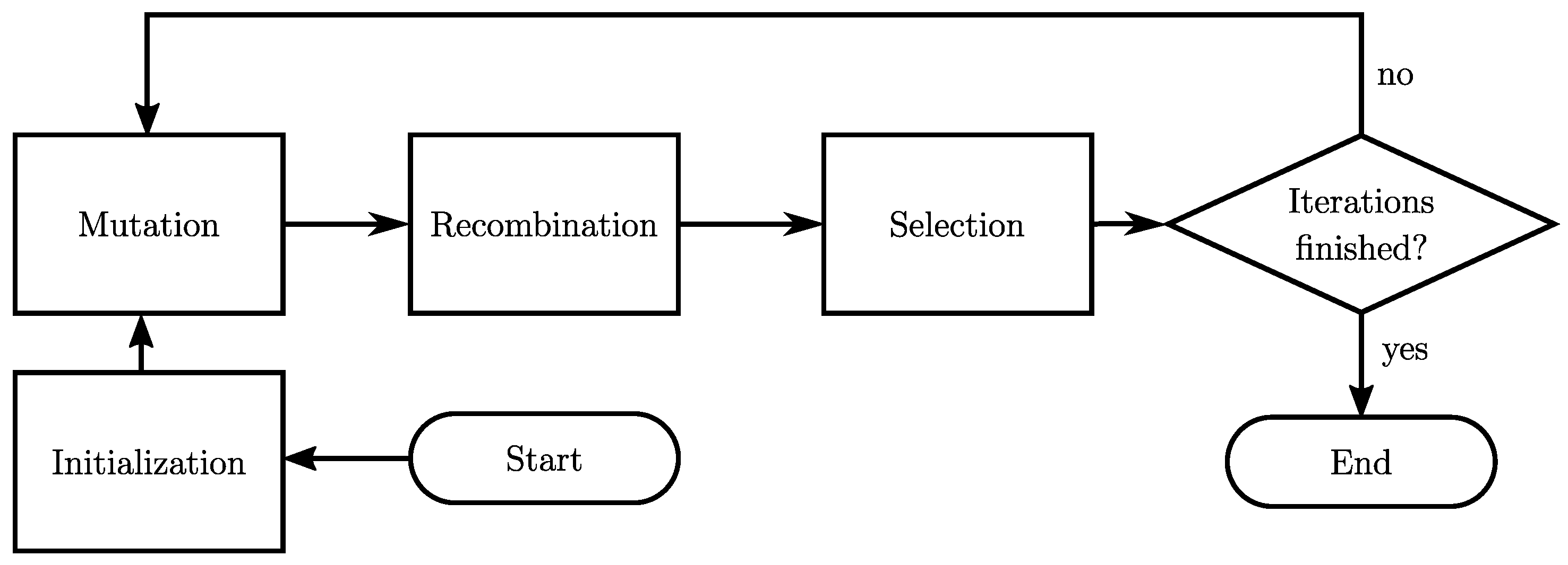
2.4. Differential Evolution

DE is an evolutionary algorithm for multivariate functions optimization with many highly successful applications [13]. DE proposes a set of Candidate Solutions (CS) that compete for the best performance in the objective function $f(·)$. In Figure 2, the basic DE scheme is described.

A CS is a vector whose elements match the variables in $f(·)$. The population is randomly initialized inside predefined bounds that limit the search space. Afterwards in the mutation process, a donor vector $v_i$ is calculated for every CS $x_i$, by randomly selecting three different CSs, $\{r_1,r_2,r_3\}$ and applying (7), where F is the mutation factor $F\in [0,2]$.

$$v_i=r_1+F(r_2-r_3)$$

(7)

In the recombination process, the CS $x_i$ is recombined with the donor vector v in every dimension j to obtain a new CS $u_i$ as is shown in (8), where $rand\left(\right)\sim U[0,1]$, and $CR$ is the crossover rate.

$$u_i\left(j\right)=\left\{\begin{array}{cc}{v}_i\left(j\right)& \mathrm{if}rand\left(\right)\le CR\hfill \\ x_i\left(j\right)& \mathrm{if}rand\left(\right)>CR\hfill \end{array}\right.$$

(8)

Finally, in the selection process the new CS $u_i$ is compared to the actual CS $x_i$, and use (9) (for a minimization problem) to choose whether to keep the actual solution or replace it with the new one.

$$x_i=\left\{\begin{array}{cc}{u}_i& \mathrm{if}f\left(u_i\right)\le f\left(x_i\right)\hfill \\ x_i& \mathrm{otherwise}\hfill \end{array}\right.$$

(9)

The mutation, recombination, and selection function for a certain number of iterations is continuously performed, and ultimately, the CS with the best performance in $f(·)$ is returned.

3. Ellipsoidal Surfaces Optimization

In 2017, we presented the Hyperellipsoidal Neuron (HN) [10], where the neuron represents an hyperellipsoidal decision surface. The HN is capable of deforming the decision surface into geometric entities, such as a pair of planes, and spheres and pseudocylinders. In this paper, we use the same propagation of the HN for representing the ellipsoidal surfaces.

We use the parametrization functions ${\psi }_1(·)$ and ${\psi }_2(·)$ defined in (10) and (11) respectively.

$${\psi }_1\left(x\right)={\left[x_1,\cdots ,x_n,1,-\frac{1}{2}{x}_1^2,\cdots ,-\frac{1}{2}{x}_n^2\right]}^T$$

(10)

$${\psi }_2\left(E\right)={\left[\frac{c_1}{r_1^2},\cdots ,\frac{c_n}{r_n^2},-\frac{1}{2}\left(\frac{c_1^2}{r_1^2}+\cdots +\frac{c_n^2}{r_n^2}-1\right),\frac{1}{r_1^2},\cdots ,\frac{1}{r_n^2}\right]}^T$$

(11)

Note that the product ${\psi }_1{\left(X\right)}^T{\psi }_2\left(E\right)$ is a parameterization in ${\mathbb{R}}^{2n+1}$ of the the inner product in the algebra ${\mathbb{G}}_{2n,n}$, and by the definition of an ellipsoid in the inner product null space, it is possible to ensure that a point lies on the ellipsoid surface if ${\psi }_1{\left(X\right)}^T{\psi }_2\left(E\right)=0$.

In [10] was presented a training algorithm of HNs for classification. However, the aim of this paper is not to classify points but to approximate surfaces of cloud points with ellipsoids. Hence, in what follows, the development of a new training algorithm to solve the problem of obtaining object maps of environments is presented.

Training Algorithm for 3D Mapping

Two sets of parameters, the center $\{c_x,c_y,c_z\}$ and the semi-axes $\{r_x,r_y,r_z\}$, are adapted to represent an ellipsoid. Similar to the case of RBF networks, the ellipsoid center is trained with k-means++, taking the centroid of the cluster as the center of the ellipsoid. Then, for a point cloud with n points $\{X_1,X_2,\cdots ,X_n\}$, k clusters $\{S_1,S_2,\cdots ,S_k\}$ and k centroids $\{c_1,c_2,\cdots ,c_k\}$ for the ellipsoids are found.

For training the semiaxes, the inner product of each point and ellipsoid ${\psi }_1{\left(X\right)}^T{\psi }_2\left(E\right)$ is minimized, consequently the distance between the points and the ellipsoid surface is minimized. Additionally, the volume of the ellipsoid, defined as $V=\frac{4}{3}\pi r_x{r}_y{r}_z$, must be penalized to avoid trivial solutions, e.g., an ellipsoid contained all of the point cloud or a ellipsoid approximating just one point.

Finally, the fitness function for the DE algorithm in (12) is designed, where every cluster $S_i$, calculated by k-means++, is used for adapting the semiaxes $\{r_x,r_y,r_z\}$ of an ellipsoid with center $c_i$. The first term penalizes the distance from every point in the cluster to the ellipsoid surface (outside or inside) by applying the root mean square error (RMSE), and the second term penalizes the density of each cluster $S_i$ by computing the ratio of the volume of the entity to the number of points contained in $S_i$, i.e., $S_i$.

$$(r_x,r_y,r_z)=\underset{(r_x,r_y,r_z)}{\arg \min }\alpha \sqrt{\frac{1}{S_i}\sum _{X\in S_i}{\left[{\psi }_1{\left(X\right)}^T{\psi }_2\left(E\right)\right]}^2}+\frac{4(1-\alpha )}{3S_i}\pi r_x{r}_y{r}_z$$

(12)

The free parameter $\alpha$ controls how much the ellipsoid can grow; $\alpha$ and the parameter k control the granularity of the ellipsoidal map. The granularity refers to the number and size of the ellipsoids that represent an object.

4. Experiments

To show the capabilities of the proposed algorithm, in this section, the results of experiments are presented. For all of the following experiments, DE is used with parameter settings: $F=1.2$ and $CR=0.7$ and a fixed population of 10 particles and 50 iterations. The objective function has the parameter $\alpha =0.8$, that was chosen heuristically for a good granularity balance. The point clouds are provided by an SRI-500 Laser Rangefinder from Acuity Technologies capable of scanning 800,000 points per second at distances of up to 500 feet (150 meters approximately).

4.1. Object Mapping

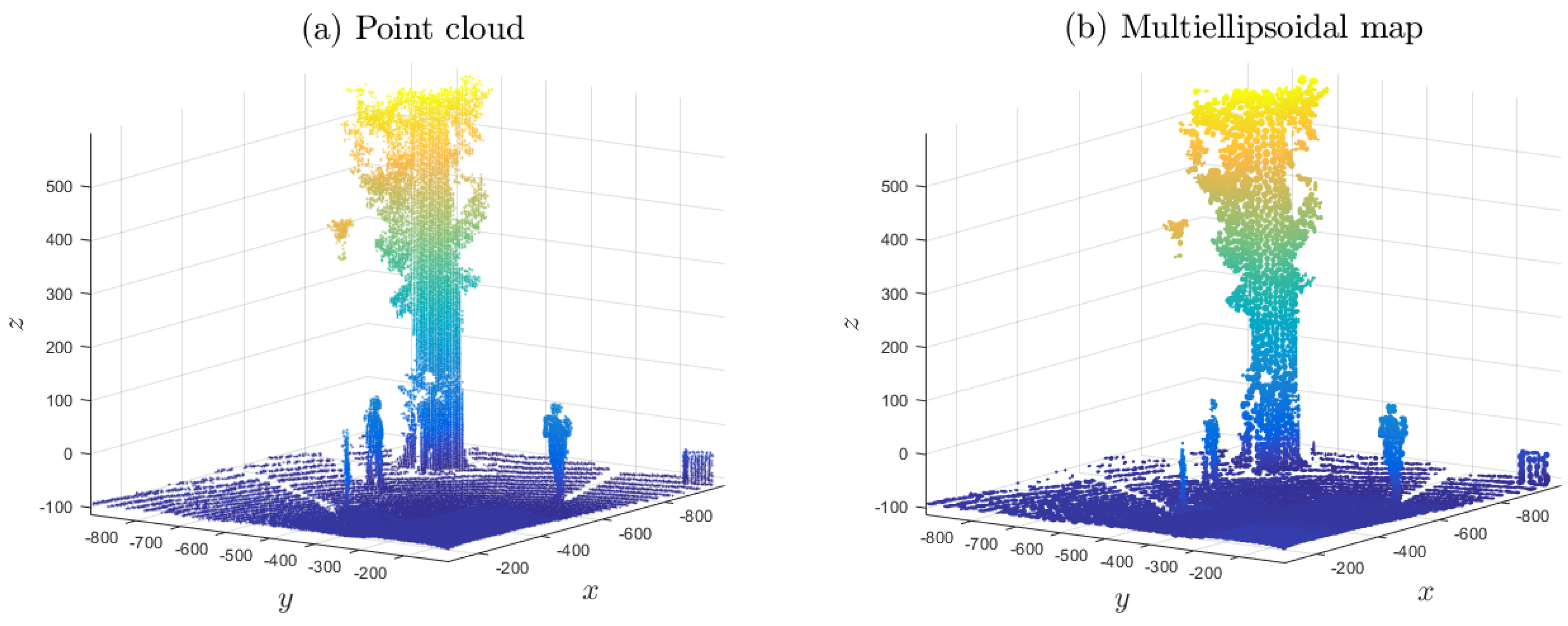
In experiment 1, as shown in Figure 3, the point cloud (left) is composed of 10,916 three-dimensional points and the multiellipsoidal map (right) contains 150 ellipsoids.

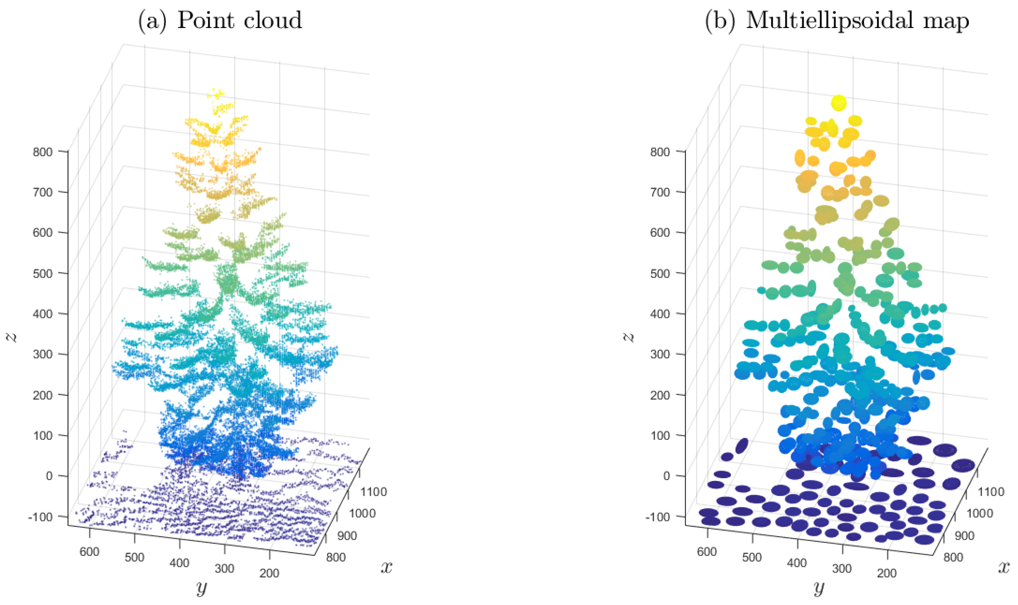
Similarly, in experiment 2, shown in Figure 4, a map of a tree of 31,049 points is adapted with 400 ellipsoids. Notably, the ellipsoids that are on the floor of the approximation are projected onto the 2D plane defined by the x and y axes of the figure.

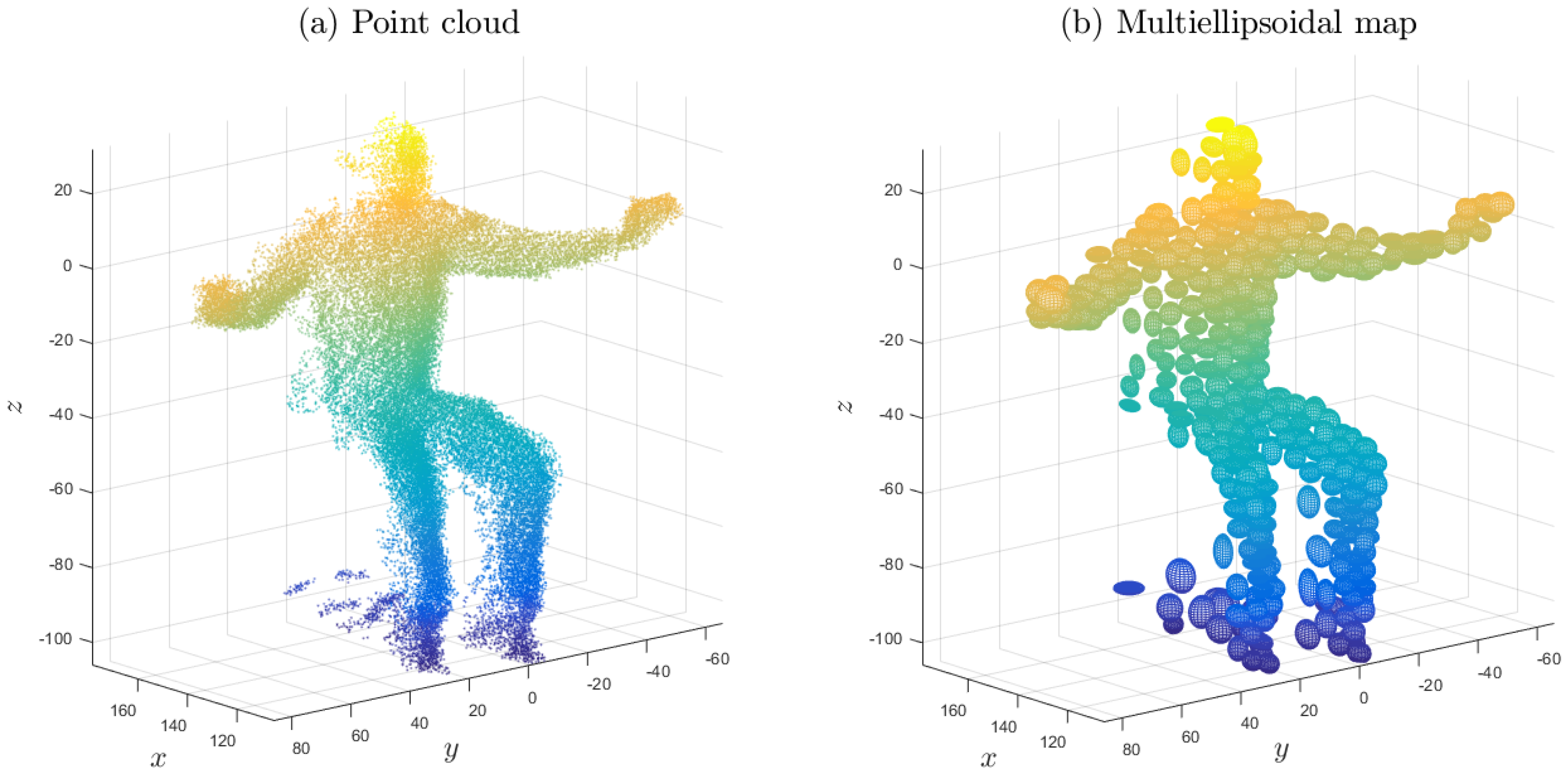
In Figure 5, the results of experiment 3 are shown. This is an example of a person with opened arms. As can be seen, concave areas are represented accurately by several ellipsoids. The point cloud has 40,883 points, and the multiellipsoidal map contains only 350 ellipsoids.

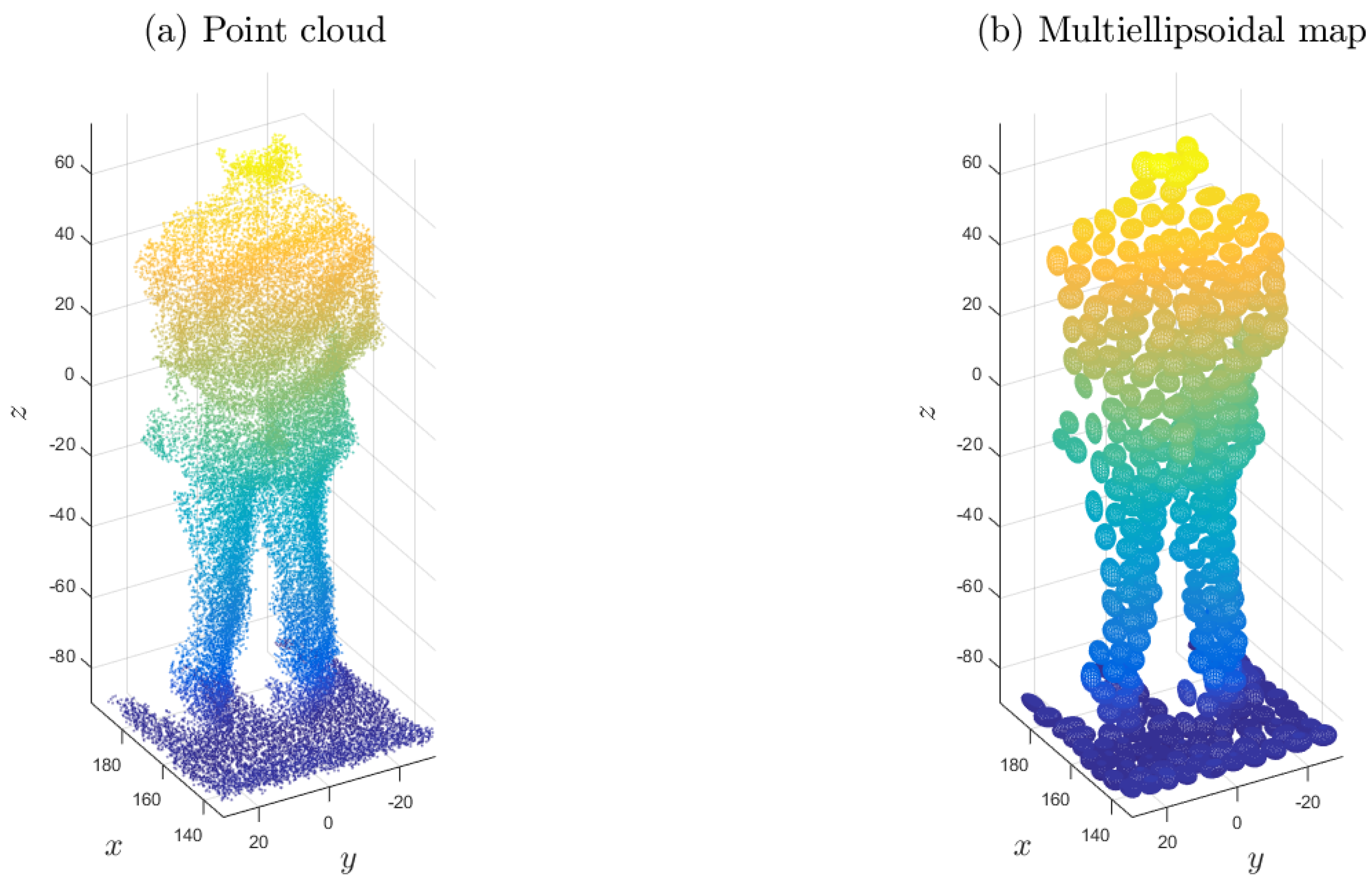
In experiment 4 in Figure 6, a man is standing with his back toward the observer. The point cloud is formed by 37,142 points, and the multiellipsoidal map contains 350 ellipsoids.

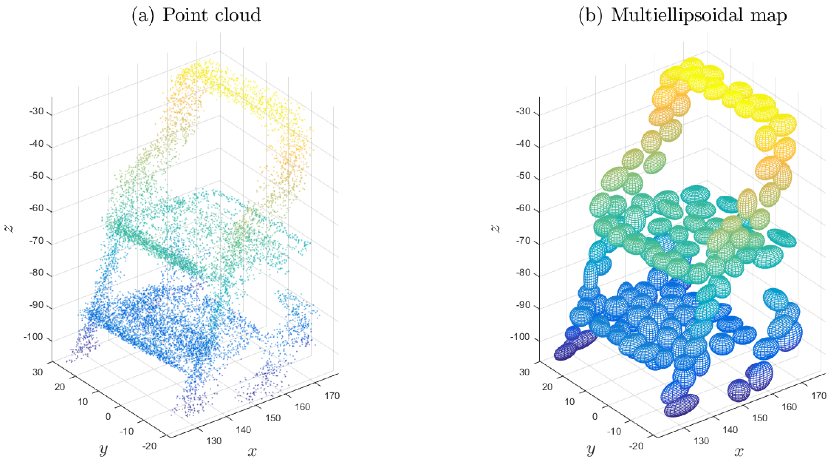
In Figure 7, another human figure is considered, in this case, a man with open arms sitting in a chair. The point cloud is formed by 42,272 points, and the multiellipsoidal map has 350 ellipsoids.

Summarizing these five experiments, it is observed that a good approximation and representation of the objects are obtained even when a small number of ellipsoids is used.

Table 2. Memory cost of the representation—part 1.

Experiment	Point Cloud		Multiellipsoidal Map		Percentage Cost
	Points	Bytes	Ellipsoids	Bytes
Experiment 1	10,916	130,992	150	3600	2.7482%
Experiment 2	31,049	372,588	400	9600	2.5765%
Experiment 3	40,883	490,596	350	8400	1.7122%
Experiment 4	37,142	445,704	350	8400	1.8846%
Experiment 5	42,272	507,264	350	8400	1.6559%

shows the memory cost. Consider a four-byte floating-point number; then, the memory cost of the cloud point (three floating-point numbers for each point) and of the multiellipsoidal map (six floating-point numbers for each ellipsoid) is calculated. Finally, a percentage cost of each map is shown, where it is easy to observe that an information-rich map with low memory cost has been obtained.

4.2. Varying the Number of Ellipsoids

The percentage cost shown in Table 2 depends on the chosen number of ellipsoids (k). To show how the representation changes with k, consider experiment 6 in Figure 8, where a point cloud of an office chair is approximated with various numbers of ellipsoids. The number of ellipsoids that are shown depends on the application.

4.3. Ellipsoid Deformation

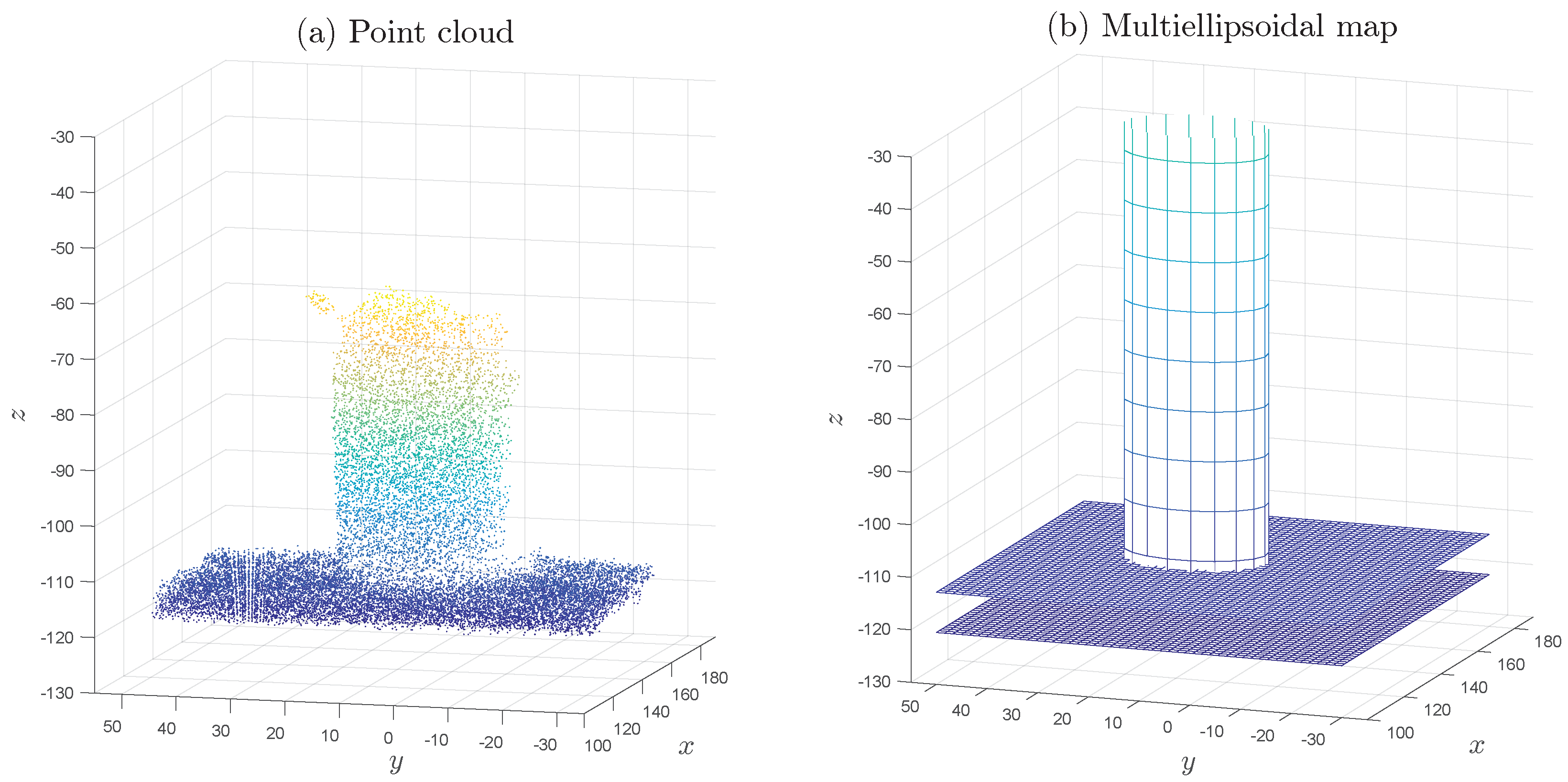
Table 1 presents the geometric entities that can be obtained when an ellipsoid is deformed using the GA framework. Figure 9 shows the results of experiment 7, where a trash can is approximated with two ellipsoids. We use a threshold of four meters for deforming the ellipsoids. It can be observed that an ellipsoid is deformed into a pseudocylinder for adapting all of the points of the sides of the trash can; additionally, to represent the floor, another ellipsoid is deformed into a pair of planes. This representation is very useful for robotic navigation; however, because a partition clustering technique is used, the ellipsoid size is also controlled by the number of ellipsoids. For a more general way of segmenting, it is always possible to choose to change to a hierarchical clustering algorithm which would allow us to obtain the mentioned deformations of the ellipsoids into pseudo cylinders or pair of planes.

4.4. Environment Mapping

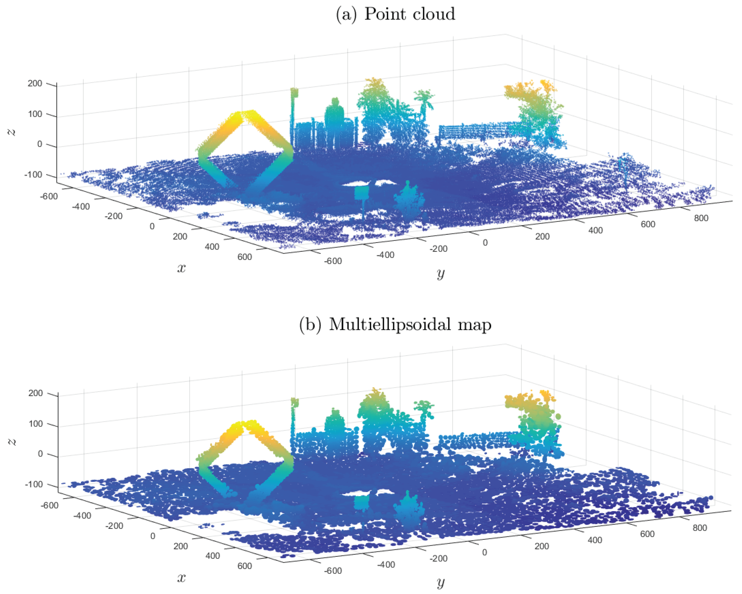
The multiellipsoidal mapping algorithm presented is useful for mapping not only for objects but also environments. Figure 10 and Figure 11 presents two experiments that show the proposed algorithm’s capabilities for mapping environments. In

Table 3. Memory cost of the representation—part 2.

Experiment	Point Cloud		Multiellipsoidal Map		Percentage Cost
	Points	Bytes	Ellipsoids	Bytes
Experiment 8	714,446	8,573,352	8880	213,120	2.4858%
Experiment 9	70,447	845,364	5920	142,080	16.8069%

, the memory cost of representing these environments is shown.

4.5. Comparison to Spherical Mapping

Multiplanar mapping algorithms have been used for many applications such as urban mapping and office-like environments representation; however, these algorithms are not suitable to mapping free form objects. To solve this problem, dense multiplanar representations have been developed [5]; however, another problem then arises because, in such cases, the planes boundaries must be defined.

Spherical mapping [8,9] solves both problems by approximating the cloud point with spheres. Because the proposed approach is an extension of the spherical mapping, both approaches are empirically compared to show that ellipsoids can more accurately represent a point cloud.

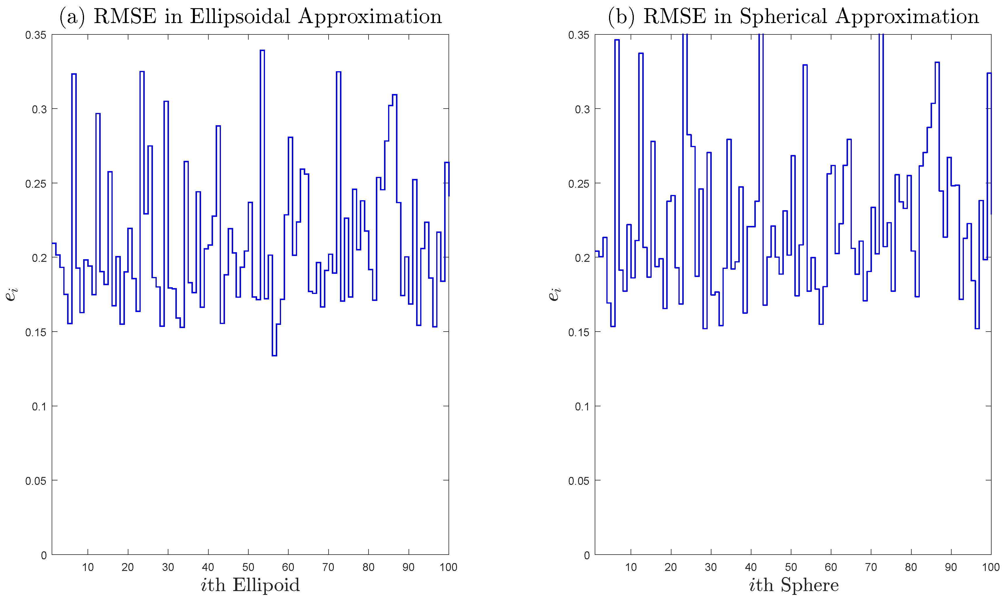
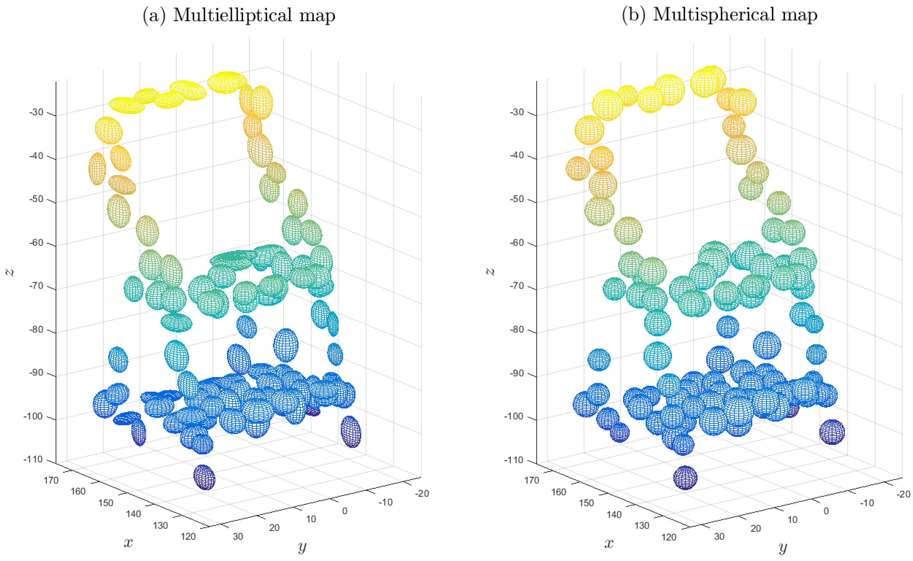
Let us consider the model error for the point cloud of experiment 1. Let $x\in S_i$ represent the points in the cluster $S_i$ and d be the closest to x three-dimensional points on the spherical or ellipsoidal surface. Then, the RMSE defined by (13) is shown, where i is the number of the cluster. Figure 12 shows the ellipsoidal and spherical approximations with $k=100$. The spherical mapping is created in the exactly same way as ellipsoidal, except for adapting only one radius.

$$e_i=\sqrt{\frac{{\sum }_{x\in S_i}{(d\left(x\right)-x)}^2}{S_i}}$$

(13)

In Figure 13, we present the histograms of error of the ellipsoidal and the spherical approaches. In the left, the error $e_i$ calculated using Equation (13) of each ellipsoid is shown. In the same way, in the right we have the calculated error for each sphere. In

Table 4. Errors of ellipsoidal and spherical approximations.

Approximation	Mean	STD	Maximum	Minimum	Total
Ellipsoidal	0.2079	0.0451	0.3604	0.1351	20.7936
Spherical	0.2258	0.0540	0.4647	0.1475	22.5769

, their statistical measures are provided.

Note that the multiellipsoidal mapping has a smaller error than the spherical representation due to the degrees of freedom of the ellipsoid. Hence, in this experiment, it has been empirically shown that the ellipsoidal mapping represents an improvement in the spherical mapping algorithm.

5. Discussion of Other Mapping Algorithms

In this section, the differences between mapping algorithms based on the approximation of geometric entities and those based on function approximation are discussed; in particular, the difference between the approximation of geometric entities represented in GA as multivectors [6,7,8,9] and approximations of functions such as the Gaussian approximation with RBF networks [3] or generalized distance functions [4].

5.1. The Best Approximation

Regarding the best approximation, the RBF is a successful technique because, in similarity with the Multi-layer Perceptron, the universal approximation theorem [21] shows that RBF can be used for approximating any free form object. However, there is no theorem that shows that planes, spheres, and ellipsoids are in fact universal approximators. Consequently, it is possible to claim that the approximation of functions will result in the best fit of the point cloud. This is a good property if the application is point cloud interpolation.

5.2. Compactness and Heuristics

As can be seen, function approximation results in the best approximation; however, because functions with the domain $(-\infty ,\infty )$ are considered, such functions have to be bounded, and a heuristic is needed to determine the plane position (and the points transformation) where the 3D function is defined. This problem implies that more parameters for the approximation must be used. In contrast, using geometric entities of GA, self-bounded entities such as spheres and ellipsoids and infinite entities such as pseudocylinders, planes, and pairs of planes are obtained. Additionally, because all the entities belong to the same algebra and the geometric locus is defined by their null space, heuristics to fix the representation are not required. Hence, we conclude that geometric entities are useful for easy implementation and compactness. We can also argue that the best information compression can be obtained as shown in Table 2, Table 3 and Table 4.

5.3. The Best Mathematical Framework

For most robotic applications, obtaining the map is merely an initial step. Hence, it is important that the map be suitable for subsequent tasks. In the case of functions, it is computationally expensive to apply a rigid transformation as is needed in many applications. In contrast, geometric entities represented by multivectors are suitable for such transformations, because the same operators can be used in every entity. These features make GA suitable to pose estimation [15], movement estimation [16], navigation over rough terrain [14], computation of inverse kinematics [22], object manipulation [23], 3D reconstruction of buildings [6], and other applications in computer graphics [24]. In conclusion, the mapping algorithms based on GA offer a suitable framework for algorithms development.

6. Conclusions

In this paper, a new mapping algorithm based in ${\mathbb{G}}_{6,3}$ GA has been presented, capable of adapting multiples ellipsoids to obtain an object representation that is more compact than the point cloud. This multiellipsoidal mapping offers information-rich maps suitable for representation and approximation at low memory cost. Furthermore, the use of the GA framework allows us to work with an algebraic representation of ellipsoids that is capable of deforming the ellipsoids by themselves into other quadratic surfaces, such as spheres, pair of planes and pseudocylinders; this feature is valuable for robotic mapping.

As our results show, compared to other object-mapping algorithms like multiplanar mapping [5] and spherical volume registration [8,9], ellipsoids could adapt better free form objects. In the Section 5, we discussed that in contrast to mapping algorithms based in RBF [3] or other functions [4], the ellipsoid is an element of GA ${\mathbb{G}}_{6,3}$, and is hence easier to manipulate than functions. This property will provide a better framework for other robotic tasks such as path planning and navigation.

7. Future Work

The proposed algorithm is strongly related to the clustering algorithms that segment the cloud point to get other quadratic surfaces; a hierarchical clustering methodology is necessary. This improvement will reduce the number of geometric entities. Consequently, no k parameter should be found.

The presented algorithm can also be abstracted as a one-layer neural network consisting in HNs. The extension of this neural network could be trained for on-line capabilities (e.g., trained with Extended Kalman Filter), this could lead to a dynamic multielliptical mapping algorithm. Furthermore, the parameters k and $\alpha$ were selected heuristically; for a better understanding of how these parameters affect the granularity of the mapping algorithm, a new study has to be done.