Quantitative Deterioration Assessment of Road Bridge Decks Based on Site Inspected Cracks

1
Department of Civil Engineering, The University of Tokyo, 7-3-1 Hongo, Bunkyo-ku, Tokyo 113-8656, Japan
2
Department of Civil and Environmental Engineering, Kanazawa Institute of Technology, 7-1 Nonoichi 921-8501, Japan
3
Institute of Advanced Sciences, Yokohama National University, 79-1 Tokiwadai, Hodogaya, Yokohama 240-8501, Japan
*
Author to whom correspondence should be addressed.
Appl. Sci. 2018, 8(7), 1197; https://doi.org/10.3390/app8071197
Submission received: 20 June 2018
/
Revised: 4 July 2018
/
Accepted: 18 July 2018
/
Published: 21 July 2018
(This article belongs to the Special Issue Modelling of Early Age Cracking Risks and Serviceability of Concrete Structures)
Abstract
:By integrating a multi-scale simulation with the pseudo-cracking method, the remaining fatigue life of in-service reinforced concrete (RC) bridge decks can be estimated based upon their site-inspected crack patterns. But, it still takes time for computation. In order to achieve a quick deterioration-magnitude assessment of RC decks based upon their crack patterns, two evaluation methods are proposed. A predictive correlation between the remaining fatigue life and the cracks density (both cracks length and width) is presented as a fast judgment. For fair-detailed judgment, an artificial neural network (ANN) model is also introduced which is the basis of the machine learning. Both assessment methods are built commonly by thousands of artificial random crack patterns to cover all possible ranges since the variety of the real crack patterns on site is more or less limited. The built ANN performances are examined by k-fold cross-validation besides checking the prediction accuracy of real crack patterns of bridge RC decks. Finally, the hazard map of the deck’s bottom surface is introduced to indicate the location of higher risk cracking, which derives from the estimated weight of individual neuron in the built artificial neural network.
1. Introduction
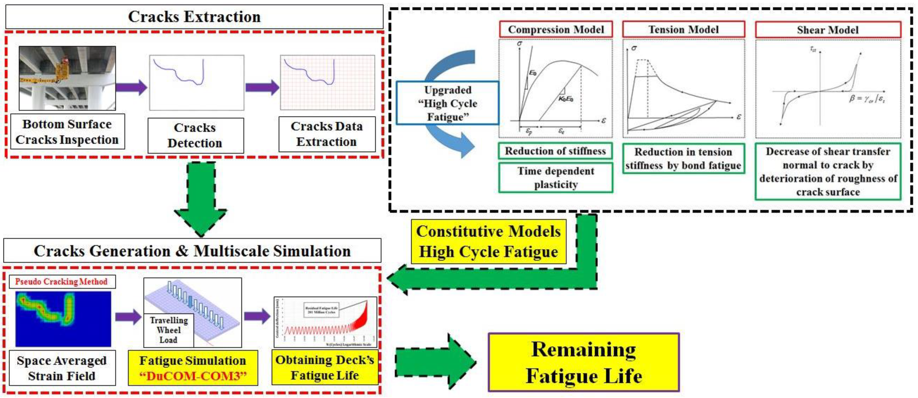
In the renewal projects of highways, it is estimated that more than half of total maintenance cost will be spent for the renewal and repair of bridge decks [1] and cost reduction in the maintenance of bridge decks is a crucial matter. Remaining fatigue life is essential information to conduct a reliable maintenance plan. Crack grading by visual inspection is used to categorize the degree of deterioration [2]. However, this grading method is not able to estimate the remaining life quantitatively. Here, one of the technologies to assess the fatigue life is a multi-scale simulation [3,4]. By introducing the time-dependent constitutive models into the multi-scale simulation program, fatigue life of bridge decks can be predicted numerically [5]. Furthermore, the integration of inspection data with the life-simulation (pseudo-cracking method) can upgrade the reliability of life estimation of existing bridge deck [6,7] as shown in Figure 1. As the multiscale simulation deals with the geometric crack patterns, it requires huge calculation cost. Thus, the authors try to utilize the artificial intelligence in order to achieve the remaining fatigue life in just a moment with running complex multiscale simulation.
In the data assimilation technology [8,9,10], crack patterns observed on lower faces is induced into the life-simulation analysis as an initial state of damages for the future simulation. Lucked defect information is complemented by the predictor-corrector iterative search of energy based stability. Based on the data assimilation technology, the authors present two evaluation methods in this study for the deterioration-magnitude assessment of reinforced concrete (RC) decks which are derived from their inspected bottom surface cracks. One is the statistical model to correlate the remaining fatigue life versus the crack density. Thus, the parameter used has clear physical and mechanical meanings to be easily understood.
The other one is the artificial neural network model of a machine-learning basis. Contrary to its great versatility, the physical and mechanical structures of the network are difficult to be understood, theoretically and mechanically. But, it is expected that the built neuron network may have an implicit similarity to the risk of cracking on the remaining fatigue life. Then, it is thought by the authors to be meaningful to compare both methods of different approaches.
As the first step, the remaining fatigue life of in-service existing decks is examined in reference to real crack patterns of a wide variety by utilizing the life assessment technology developed previously. Thus, we check the range of the fatigue life with regard to the real crack patterns and it will be used at the final step to secure the generalization of the proposed ANN model. Here, it should be noted again that the authors apply artificially made crack patterns for building both the statistical and AI models. This is to compensate for the limitation of available crack patterns on which the model is based and it is a highlight of this study. Randomized artificial crack pattern program (RACP) is introduced to build the evaluation models to cover all possible ranges of fatigue life. The real crack patterns will be used only for the validation of the proposed ANN model since the final objective is to check the deterioration-magnitude corresponding to real crack patterns on site.
Second, on the basis of the simulation results, an accurate correlation is proposed between the remaining fatigue life and a mechanics-based parameter of the bottom surface cracks (cracks length and width), where it can be used as a fast-truck judgment of the degree of deterioration of the decks.
Third, the authors further challenge an artificial neural network model (ANN) for fair-detailed assessment of deterioration-magnitude. This method has the advantage to be able to handle the geometrical patterns which consist of massive numbers of cracking. Bayesian regularization technique is conducted to the ANN’s training, where it may ensure the generalization and eliminate the incorrect assessment due to overlearning. Then, k-fold cross-validation is conducted to check the generalization and the robustness of the proposed model. Moreover, independent real crack patterns datasets are used to check the robustness of the trained ANN among unknown data.
The proposed evaluation methods may secure a quick diagnosis of the deterioration-magnitude of RC bridge slabs by applying just the inspected bottom surface cracks without time-consuming calculation on site. In fact, the quick judgment of remaining life at the site is crucial especially for on-site management at the emergency time.
ANN is a simple analogy of estimation process and it is recognized that the built network structure does not reflect the physics. However, it may lead to some hints or foresight for the unknown events. The authors will try to seek for physical or mechanistic principles from ANN at the final part of this research. On this line, the hazard mapping of the deck’s bottom surface is introduced to indicate the location of higher risk cracking, which derives from the estimated weight of individual neuron in the built artificial neural network.
2. Artificial Neural Network
Artificial neural network (ANN) is said to be analogous to biological nervous system structures [11,12,13,14]. It consists of a huge number of neurons to take part in individual data processing. These neurons are inter-connected at synapses to transfer signals from one to another. In general, the artificial neural network is built with (1) the input neurons, (2) the neurons arranged in hidden layers to process the information and (3) the neurons to generate the output. An artificial neuron is further formed with inputs, summation and activation blocks and only one output. The neurons in different layers are also inter-linked and each connection has its own weight which may change in accordance with the learning procedures until it achieves the expected target values.
Here, the role of the activation function is to introduce some non-linearity to the network structure so that we may treat complexity of nonlinear input-output relations. Often-used activation functions are sigmoid and hyperbolic tangent which the authors use in this paper. The role of the bias in the activation function is to provide flexibility for easy mapping of the inputs and the outputs. The output of the activation function is transferred to the connected neurons of the next layer. Each neuron works in the same way until the end layer of the network, where the expected value is compared to the output in order to check the network’s reliability. This error gap is further utilized for calculating partial derivatives with respect to the weights of each layer. Here, the weights are updated by these values. Finally, the previous steps are repeated until the discrepancy between expected targeted output and ANN’s output is minimized.
3. Building Neural Networks
3.1. Scope of Target
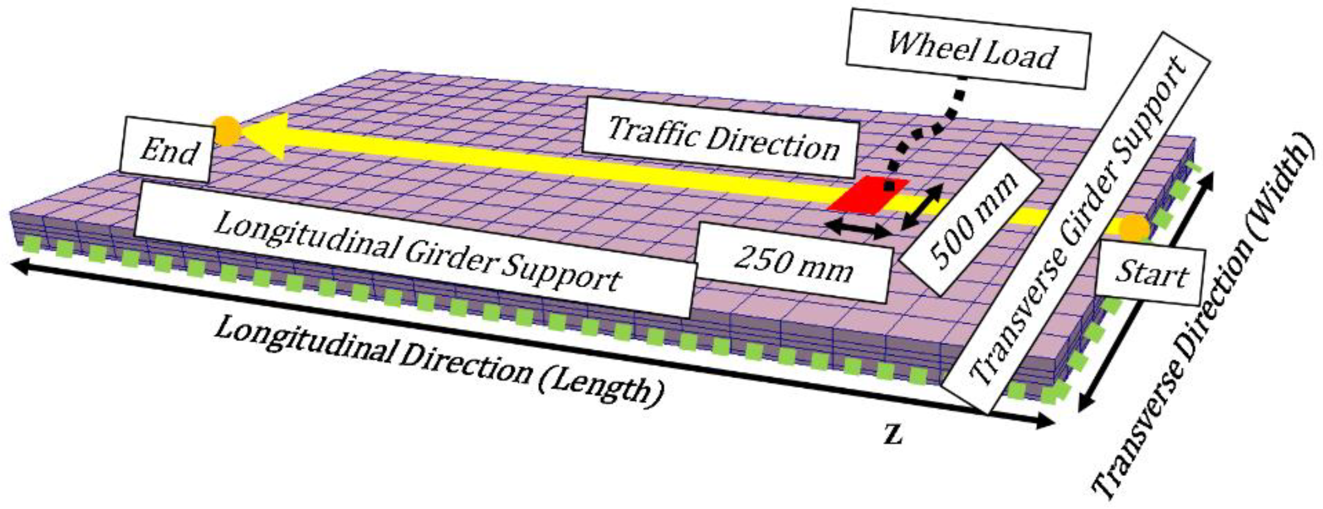
The authors direct their scientific attention to high cycle fatigue loads applied to dry RC decks of a thinner thickness less than 20 cm (see Figure 2) according to the old design codes [9,10]. For considering mechanically severe conditions, one-way single-support is set forth. For setting the necessary and sufficient length of the slab and the computation time, a sensitivity analysis was carried out in advance by checking 4.0, 6.0, 7.0, 10.0 and 15.0 m length for deciding the referential RC deck [10]. It was found that the relation of the load cycles and the center-span deflection is quite close in the case of 6.0 to 15.0 m lengths and that difference is within the acceptable range of engineering practice. Then in this paper, 6.0 m length was finally selected as a standard reference for the simulation as shown in Figure 2.
3.2. Material Properties for Reference
3.3. Loading Patterns
In reference to the Japanese standard specification for highway bridges-Part III [15], the authors set up the traveling wheel type loading of 98 kN as shown in Figure 2. Traveling speed of the wheel for simulation is decided to be 60 km/h, which is similar to the legal speed limit for Japanese national routes. In the case of fatigue loading tests, however, the running speed of the vertical load is much slower due to the mechanical limit of the testing machines. The wheel load length and the width are 500 and 250 mm in reference to the vehicle tires width, respectively.
3.4. Limit State Failure Criteria
According to the previous experiments [8], the fatigue limit state was specified in terms of the live load deflection at the center-span [16] and it is computed by assuming that the bond between concrete and reinforcement is lost in flexure. Thus, when the live load deflection defined by Equation (1) would come up to the limit state’s deflection of no bond, it is judged as the fatigue failure in association with the serviceability and safety. Then, the authors also accept this criterion so that the past research works [17,18,19] can be referred consistently. As this limit state deflection extends between (2.5–3.5) times its initial value, we apply for the criterion denoted by Equation (2) as well.
where δL,N is the central live load deflection at Nth of cycles, δ1,N is the total deflection of span center at Nth of cycles at the preceding stage of loading, δ2,N is the total deflection of span center at Nth of cycles at unloading stage, δL,0 is the initial live load deflection and Nf is number of cycles corresponding to (δL,N from Equation (2)).
3.5. Standardized States for Numerical Model
The finite element mesh, as shown previously in Figure 2, was made by the authors’ development open code [6] which is customized for the wheel running loading applied to RC bridge decks, where each mesh size is set up to be 250 × 250 mm in the X-Y in-plane and the number of layers in Z-direction of thickness is four layers.
The longitudinal supports applied to the slab are idealized line-hinges which allow free rotation but constrain the vertical displacement. In fact, RC decks are usually connected to top flanges of side steel bridge girders by studs and/or bolts. In some cases, lateral girders are also attached to stabilize the girders arranged in parallel. Then, some flexural moment constraint may exist. But, its magnitude depends upon the twist stiffness of the girders, fastening devices in detail and so on. Then, the authors set up the most explicit and conservative boundary conditions to give fatigue life of lower-limit boundary and are thought to be affected sensitively by crack patterns in space and their widths.
Here, it must be noted again that the objective and the scope of this study are to obtain the risk magnitude and hazard of inspected crack patterns on site with regard to the reference case corresponding to the standard designs of the past. For the fatigue life of decks whose shapes and dimensioning differ from those of the referential case of no damage, some simplified conversion is being developed for future step-up based upon the ANN assessment presented in this paper.
3.6. Crack Patterns Taken from Real Decks
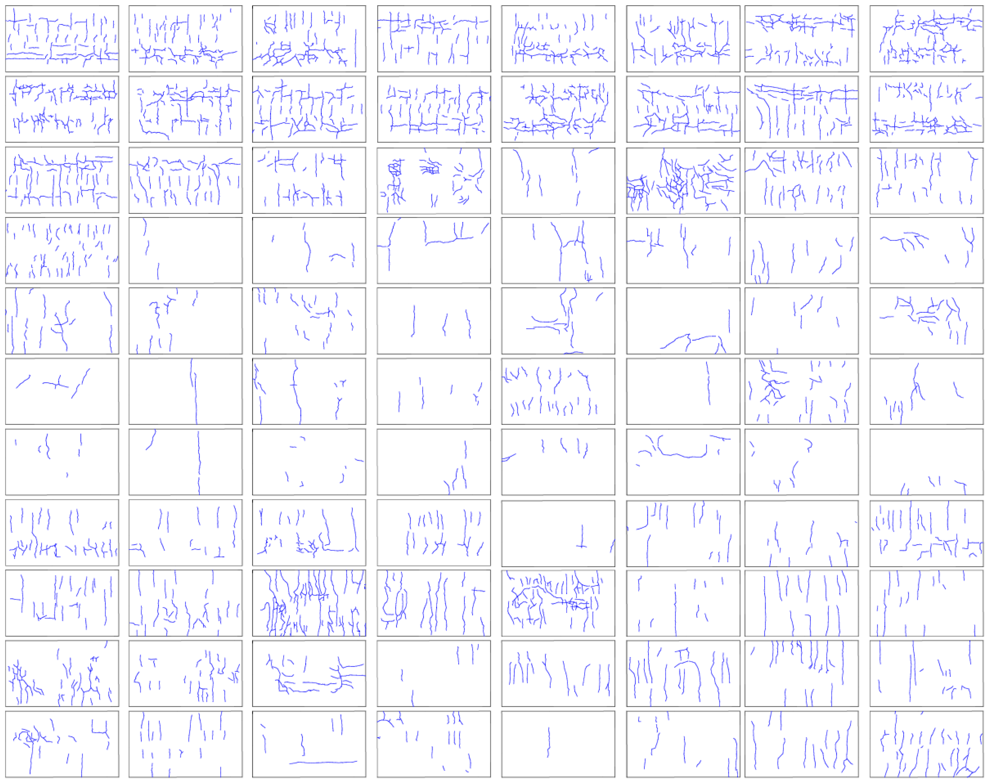
Figure 3 shows the real crack patterns reported from the on-site investigation of plenty of bridges. These are used in the life-span simulation with regard to the remaining fatigue life. A total number of 264 crack patterns with crack widths that range from 0.1 to 0.3 mm as shown in Figure 3, are investigated by using the integrated system (multi-scale simulation program & pseudo-cracking method) to obtain their remaining fatigue life [6,7,8,9]. Although the crack patterns which were actually experienced are not directly utilized in building the estimation methods, these are used only once to validate the trained ANN model stated in a later section. Thus, these will play a great important role to check the reliability of the built neural network.
Only the cracks at the bottom surface of the decks were exclusively used in the inspection data assimilation because the cracks at the top surface of in-service bridge decks are not easy to investigate on-site due to the presence of the cover of pavement in general. If the bottom surface cracks information is not enough to sufficiently estimate the remaining fatigue life, non-destructive tests (NDT) shall be applied to detect internal defects such as 3D radar system [20] and/or acoustic emission (AE) tomography [8,21,22]. The new NDTs are still under the intensive research and development [23,24]. They will be used mainly to estimate the defect at the top surface of in-service bridge decks or the internal defects.
4. Massive Life Simulation for ANN’s Learning
4.1. Referential RC Deck “No Damage”
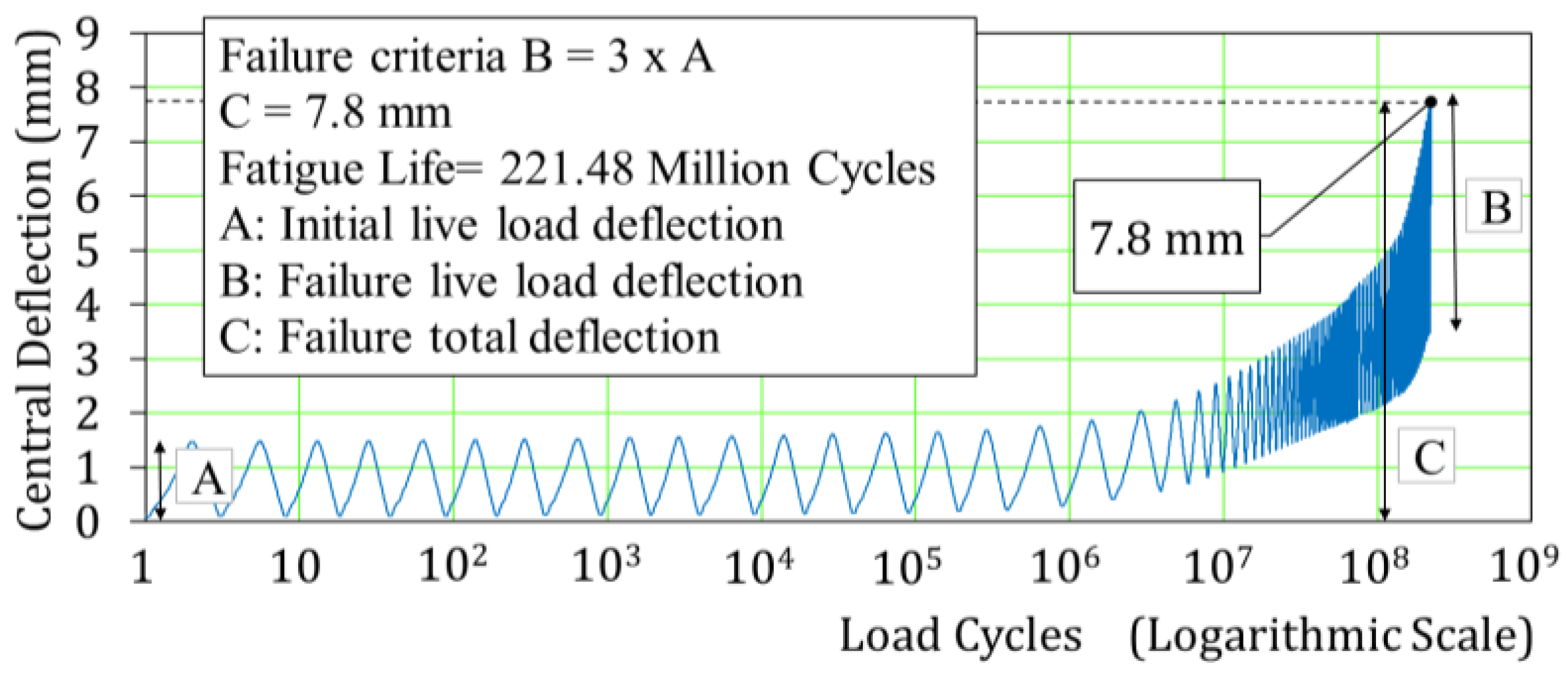
Figure 4 shows the relation of the highly repeated passage of moving wheel loads and the total deflection at span center for the referential RC deck (initially un-cracked). According to the failure criteria mentioned in the previous Section 3.4, the fatigue life of this model is estimated as 221 million cycles of passage. Here, the live load deflection at the first cycle (A) is 1.4 mm, while the live load deflection at the failure cycle (B) is 4.3 mm. Then, the total deflection of 7.8 mm was assigned as the failure one for all the studied crack patterns.
4.2. Sensitivity Analysis for Crack Depth
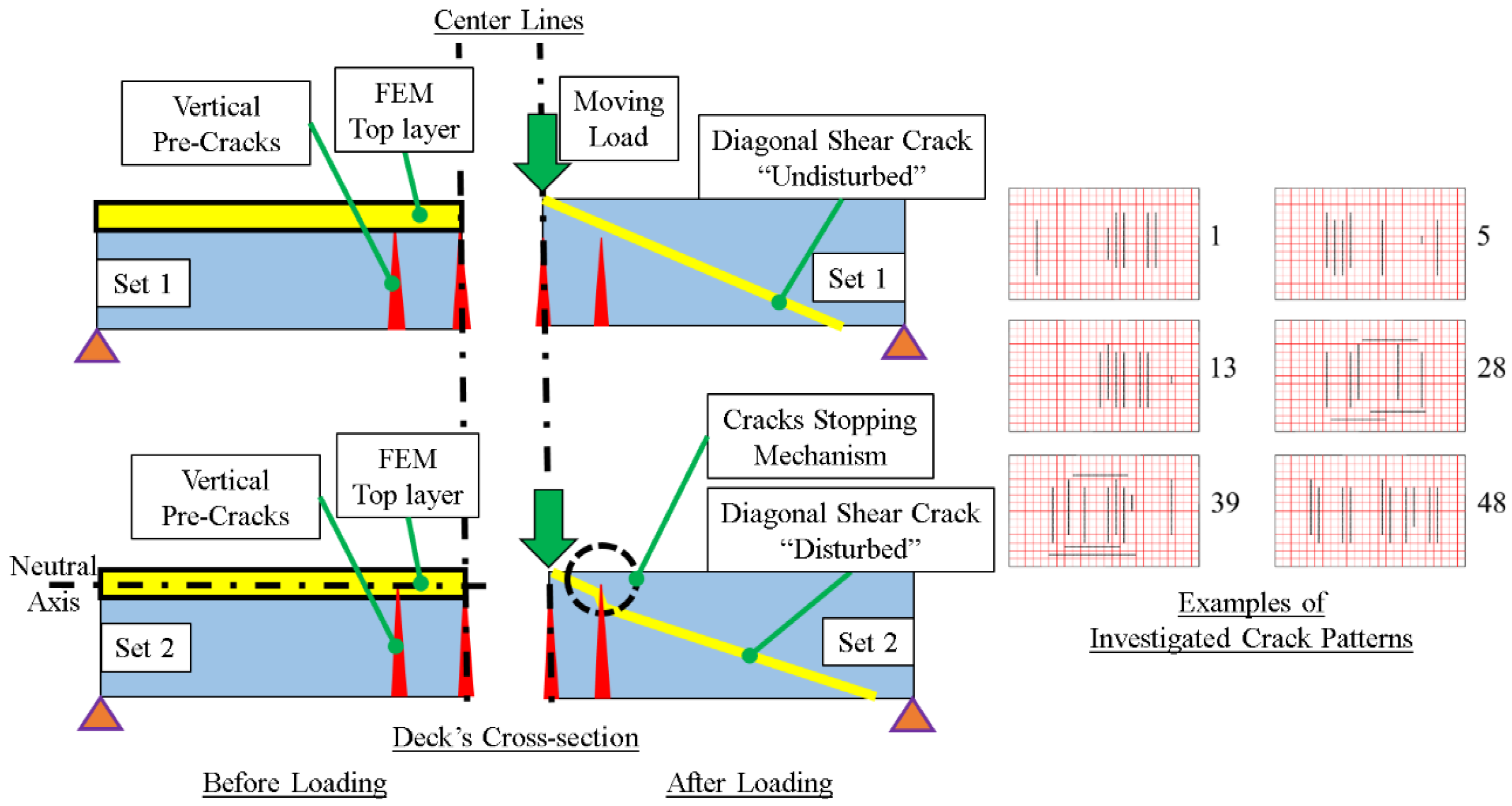
As for the preparation of the massive data processing, a sensitivity analysis was conducted to check the effect of crack depth on the fatigue life of the RC decks. Two sets of crack pattern data are arranged and each set includes the same 48 particular crack patterns as shown in Figure 5; that is, longitudinal and transverse cracks with a crack width of 0.2–1.0 mm. Here, the unique crack patterns which lead to longer life than the non-damaged reference are focused on [9,10,24]. Figure 5 shows the difference of the two sets. The pre-cracks depth of the 1st dataset does not reach the upper mesh of the FEM discretization of the RC deck (just below the lower boundary of the upper mesh), while the cracks depth of the 2nd dataset, regarding the flexural neutral axis calculations, reaches the region of the upper mesh.
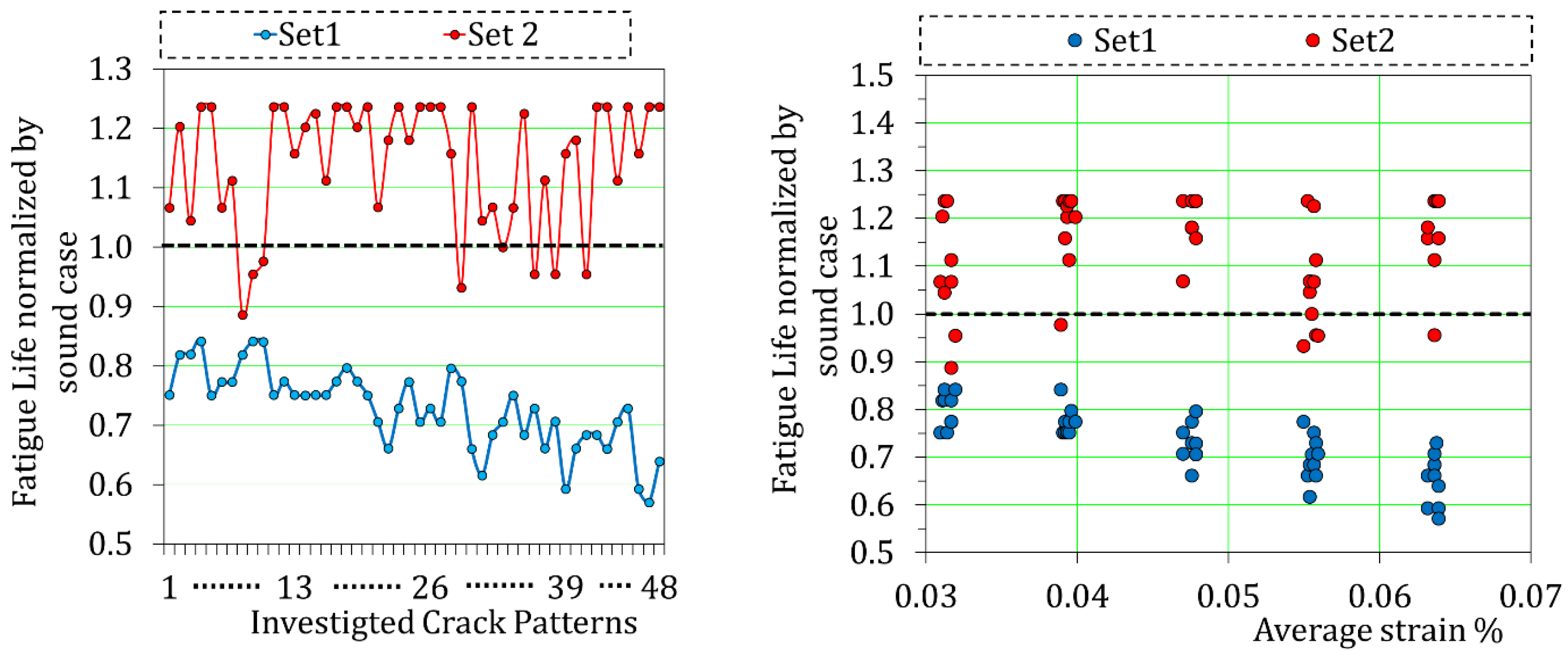
Figure 6 shows the simulation results, where the ones of all the crack patterns in the 2nd set have longer fatigue life than the same crack patterns of the 1st set but with different depth of pre-cracks. It is experimentally and analytically known [3,25,26,27] that a pre-crack stops the diagonal shear cracking when it deeply develops in advance (see Figure 5). If the depth of the pre-cracks is close to the top surface as the 2nd dataset, it disturbs the diagonal shear crack propagation and the fatigue life is prolonged.
From the above mentioned parametric study, the authors decide to treat the shallow crack depth (1st dataset) so that we may certainly get conservative but safer assessment of remaining fatigue life. When crack inspection data of both top and bottom surface cracks are available, the prediction of the fatigue life can be conducted by the same strategy presented in this research.
4.3. Cracked Cases
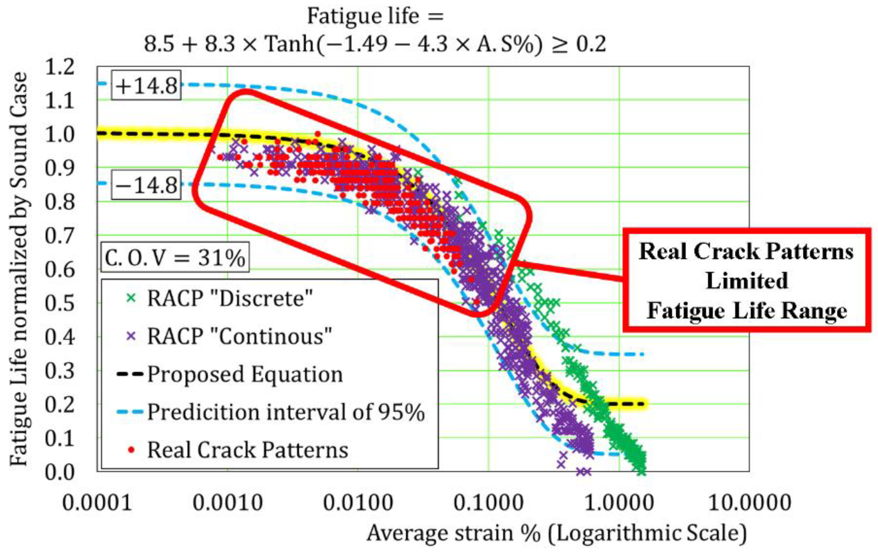
We may encounter 0.3–0.4 mm crack width as the maximum on site. Then as the first step, the authors checked the remaining fatigue life of 264 crack patterns with its width of 0.1–0.3 mm. As shown previously in Figure 3, the remaining life is obtained by the multi-scale simulation program for the real crack patterns. Figure 7 shows the relation of the average strain (see Equation (3)) and the remaining fatigue life normalized by the reference case with no initial cracking. In spite of some scatter of solution, we have the general trend as such the increasing space-averaged strains lead to shortened remaining fatigue life. The real in-service RC decks discussed here are found to have a longer life than 50% of the standard referential case. On the contrary, there are no available data of greatly shortened life whose averaged strain exceeds 0.1% or more.
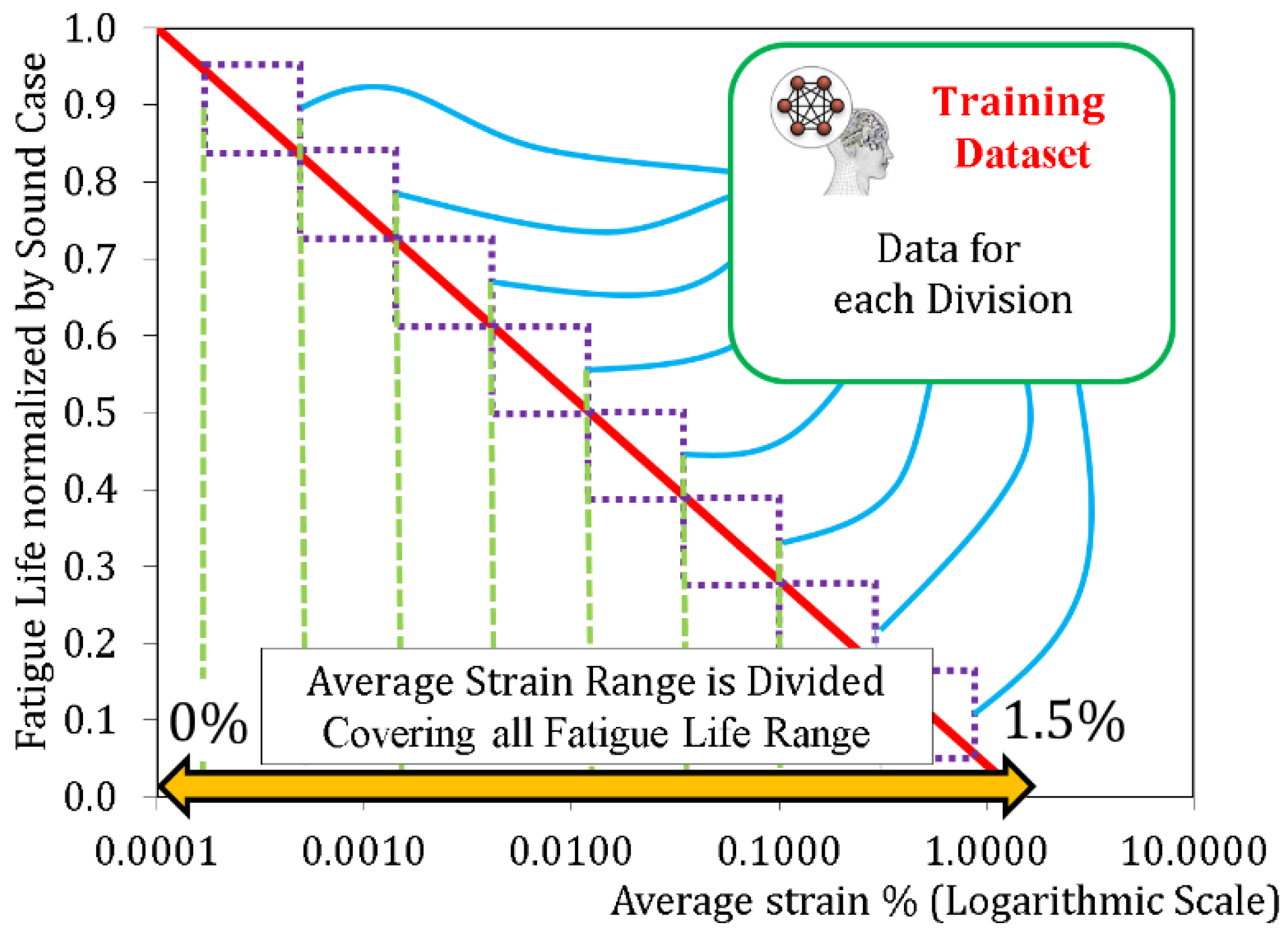
Here, it must be pointed out that the biased dataset will bring about unreliable estimation even if huge numbers of training data would be arranged. For avoiding this ill-condition, the authors computationally supply artificially produced crack patterns and their estimated fatigue strength as a part of training big dataset. To meet the challenge, we introduced randomized artificial crack patterns program (RACP) instead of gathering a huge number of real crack patterns without any criteria. As shown in Figure 8, the RC decks have fatigue life equals to one if the average strain equals to zero, while the RC decks have fatigue life equals to zero if the average strain is around 1.5% (based on a previous research [9,10]). This possible range of average strain is divided into a number of divisions, where artificial crack patterns are produced for each division to cover all possible range of fatigue life. Another reason for introducing the RACP is that the variation of real crack patterns obtained from on-site is limited. Then, it is better to use these real crack patterns only once for examining the ANN model at the final step, while the RACP will be used for building up the trained ANN model.
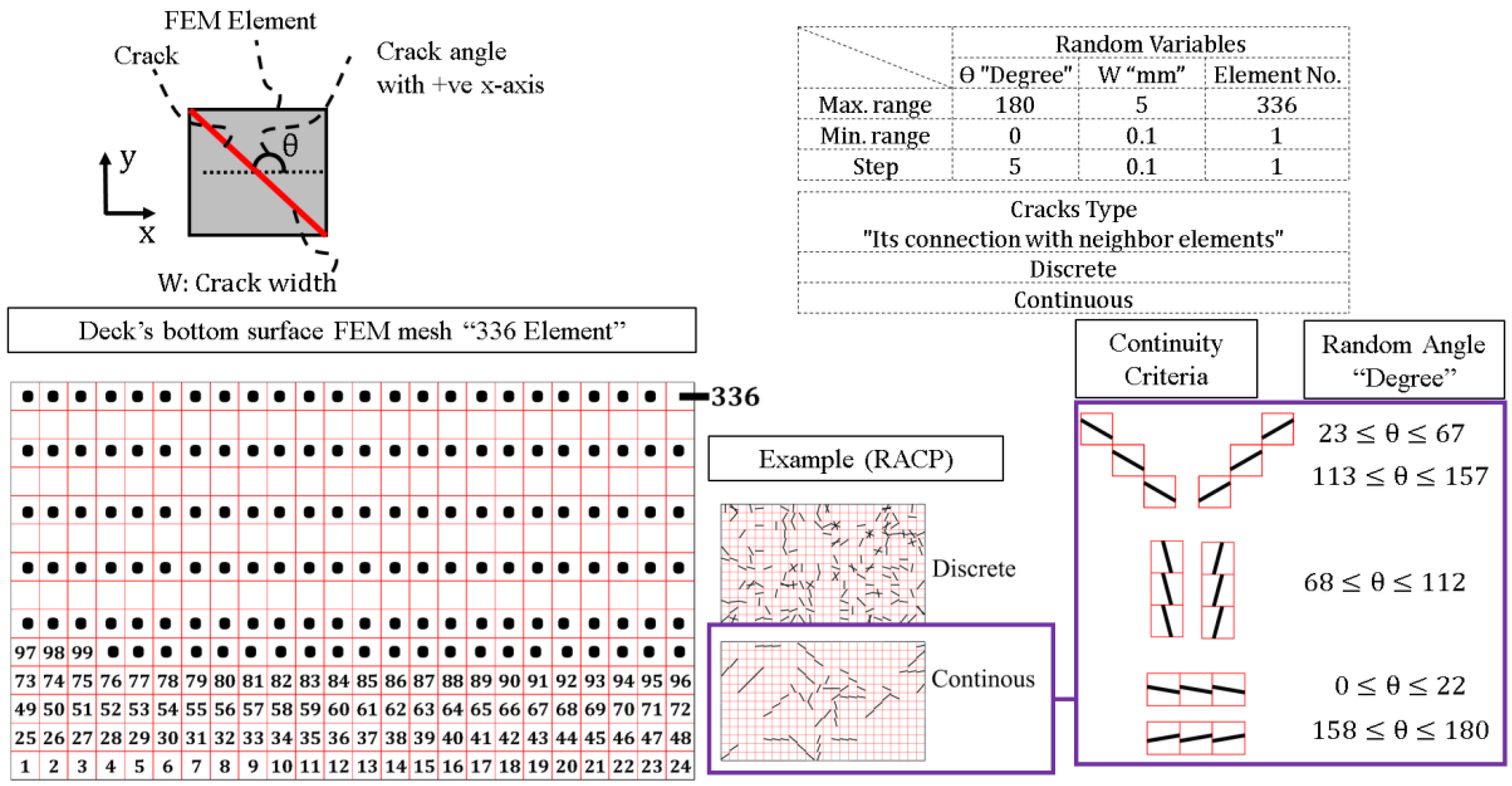
Figure 9 shows the basic idea of RACP procedure, where the random variables are the crack width, element number and crack orientation, where the ranges of randomization are 0.1–5.0 mm (step is 0.1 mm), 1–336 (step is 1) and 0–180 (step is 5 degree), respectively. Two types of cracks are produced by RACP: discrete and continuous. In the discrete cracks, there is no continuity between the crack of a particular element with the one in the neighbor elements. While in the continuous cracks, there is continuity between the crack in a particular element with the one in the neighbor elements. Based on the random angle in the continuous cracks, three shapes of continuity are produced: X-direction, Y-direction, or diagonal, as shown in Figure 9. RACP is performed based on randomization of variables and the code was made so that we may avoid repetition of cracking patterns. If it is repeated, RACP will continue randomization until a unique crack pattern is obtained.
By using the RACP, 1000 artificial random cracks were produced carefully so that it may cover all ranges of fatigue life. Two types of shapes of the cracks were set up: discrete and continuous with different length as shown in Figure 9. Their remaining fatigue life is also checked by using the multi-scale simulation. Figure 7 shows the relation of the average strain (see Equation (3)) and corresponding fatigue life normalized by the referential case for the simulation results of the artificial crack patterns. By proposing a nonlinear function for prediction, the coefficient of variation of the prediction (C.O.V) is 31% and the prediction interval of 95% is 14.8%. The results show that the fatigue life of the continuous cracks is lower than the fatigue life of the discrete cracks since the continuous cracks have more tendencies to form failure crack path.
where εavg. is the average strain on the bottom surface of RC deck, k indicates the kth element at the bottom surface of the deck, εxx is the normal strain of concrete in X-direction for the kth element, εyy is the normal strain of concrete in Y-direction for the kth element and n is the total number of elements.
4.4. Statistical Correlation of Remaining Fatigue Life and Inspected Cracks
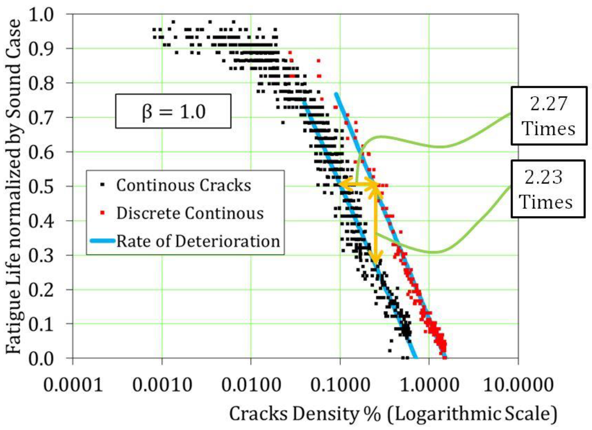
In the previous section, a correlation is found between the space-averaged strain of the bottom surface with cracks and the remaining fatigue life. For further simplicity, another statistical estimate of the life is introduced with the crack density as defined by Equation (4) in consideration of both crack length and its width. Figure 10 shows the relation of the newly introduced crack density and the normalized remaining life of RC decks under the standardized referential load. The degree of variation is similar to the one of the previous Section (average strain basis). Although the deviation of the estimated fatigue life for the discrete cracks is different from those of the continuous ones, the rate of deterioration is found to be almost the same. Thus, the factor is introduced in the definition of crack density parameter.
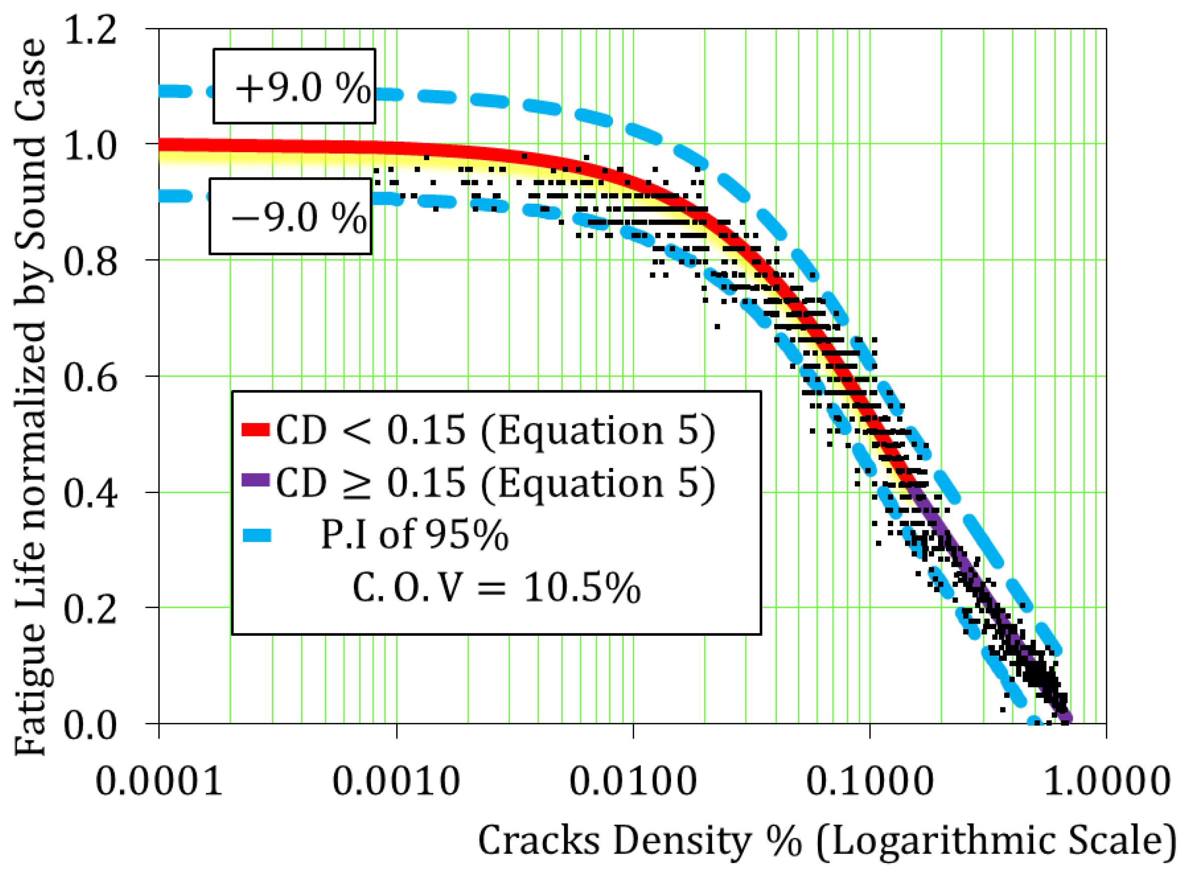
It is found that the discrete cracks defined in Section 4.3 lead to a longer life by around 2.23 times than the case of continuous cracks even in the case of the same crack density. This difference is reflected by 2.27 times difference in the crack density. Therefore, the crack density parameter can be enhanced to treat the discrete cracks by decreasing their crack density by a reduction factor ( Finally, a nonlinear formula (see Equation (5)) is proposed as shown in Figure 11, where the C.O.V of the prediction and the prediction interval (P.I) of 95% are 10.5% and 9%, respectively. The proposed correlation can be used as a fast judgment for the magnitude of deterioration of RC decks with acceptable accuracy. However, for fair-detailed judgment, cracks location and orientation should be introduced in the original computational prediction.
where CD is the crack density of the bottom surface, Lk is the length of the kth crack at the bottom surface of the RC deck and Wk is its width, A is the length of the RC deck in the longitudinal direction and B is its width in the transverse direction and β is crack type indicator; 1.0 for continuous crack and 0.44 for discrete one.
where RL is remaining fatigue life and CD is the crack density.
RL = 8.5 + 8.3 × Tanh (−1.49 − 4.6 × CD) → CD < 0.15%
= − 0.266 × ln (CD) − 0.095 ≥ 0 → CD ≥ 0.15%
= − 0.266 × ln (CD) − 0.095 ≥ 0 → CD ≥ 0.15%
5. Training Artificial Neural Networks
The crack location and its direction are factors of importance to statistically upgrade the predictive accuracy of the remaining fatigue life as discussed previously. In this section, artificial neural network (ANN) model is also presented to investigate the data processing of the massive inspection data in view of the accuracy. Especially, ANN has an advantage to directly handle geometrical information of 2D and 3D extent. The dense and sparse information of cracking is processed by ANN in terms of the sensitivity of individual neuron assigned to each location of the deck. It is rather local and discrete. On the other hand, the statistical model is formed based upon the mechanics-based parameters. Then, it is rather non-local and integrated. Comparison of both models is expected to bring about a view of massive inspected data processing.
5.1. Methodology for Fatigue Life Identification
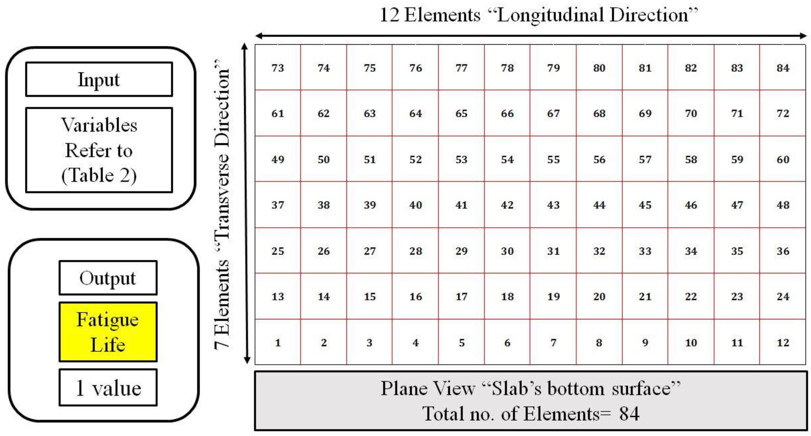
It should be noted that the performance of built ANN is dependent on the quality and quantity of the training dataset [10]. Then in this section, several cases ANN’s input variables for the same cracks information of the training dataset are arranged so as to judge the requirement on what sort of inspection dataset shall be prepared for better training. Table 2 shows four cases of the input variables of the investigated crack patterns. For case (1) & (2), the bottom layer of the finite elements is further discretized into 336 sub-elements in X-Y in-planes of 2D extent, as shown previously in Figure 9. In the data assimilation procedure [10], each sub-element has three variables, that is, normal strains in X and Y-directions (εxx, εyy) and the shear strain (εxy). For cases (3) & (4), the number of sub-elements of the deck’s bottom surface is intentionally reduced from 336 (see Figure 9) to 84 sub-elements (see Figure 12). The cracks information for case (3) & (4) is taken as a lump sum for each 500 × 500 mm2 area instead of 250 × 250 mm2 of the deck’s bottom surface.
where ε1 is the maximum principal strain, θ is its principal directional angle (degrees) and εij is the strain tensors of concrete on the bottom surface of the RC deck.
The dataset for both training and validating ANN is created by the multi-scale simulation and they are the input of the machine learning block as well. The training data is used to adjust the weights of the individual neuron of the ANN and the test dataset is used only once after the training is finished to check the validity of the training. After training the dataset in the machine learning block, if the ANN can correctly map the training data and identify the testing data, it is considered as a fairly built ANN. At last, the remaining fatigue life can be obtained for any new crack pattern in just a moment without the need for conducting any complex multi-scale simulation.
5.2. Requirements of Training Dataset
In fact, the training dataset to serve ANN has to be chosen carefully to cover all probable events which may occur in future. Once one of the events would not be supplied into the training dataset, the accuracy and reliability of the model prediction will be lost seriously [10].
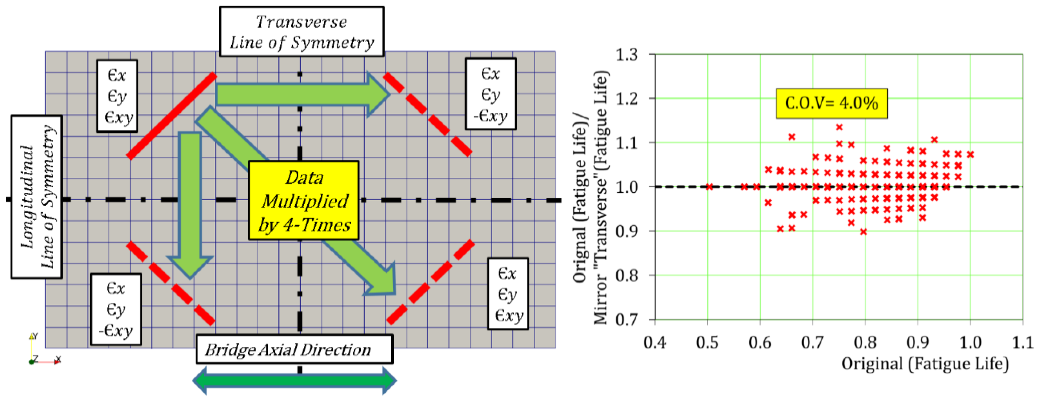
As the symmetric patterns of cracking along the traffic direction must have the same performance, the “mirror crack patterns” logically have the same remaining fatigue life as the original. So, they must be included in the training dataset as well. However, the symmetric line in the transverse direction has the different story. It is affected by the traffic direction, where the two crack patterns in the transverse direction give different remaining fatigue life [10]. The authors tried to check the remaining fatigue life of the transverse mirror crack patterns for verification (Figure 3).
Figure 13 shows how differently the transverse mirror crack patterns produce the life. As C.O.V reaches just 4%, it is negligible from an engineering viewpoint and the mirror crack patterns in the transverse direction are also included in the training dataset. Then, any dataset is multiplied by four by considering the axes of symmetry in both transverse and longitudinal directions.
In general, real cracks have their width that is not greater than 0.3–0.4 mm. Then, the authors computationally produce greater crack width up to 5.0 mm as well to compensate for the lack of inspected data at the site and to fill up the missing zone of data. As stated previously, ANN model will be built based on the artificially made crack patterns. The reason for these decisions is to secure the prediction of any unexpected events regarding rarely experienced strange crack patterns or the greater crack width that may happen in the future and to extend the range of application of the prediction. Here, the numerical analysis based on the pseudo-cracking data assimilation [8,10] is utilized to enhance the quality of inspected dataset.
5.3. Neural Network Platform and Structure
The platform used to conduct ANN algorithm is MATLAB R2017a-Neural Networks Toolbox. Unidirectional feedforward network and Bayesian regularization training function are selected for conducting the ANN [13,28,29,30,31,32,33]. The structure of the conducted ANNs is summarized in Table 3, where the input variables are discussed in Section 5.1. It should be noted that the ANN’s structure is chosen to achieve the best performance and to avoid overfitting of ANN’s model, where the size of the network should be optimum. Finally, five ANN’s models are built for the input variables’ cases based upon their optimum size of network.
5.4. Built ANN’s Performance and Input Variables
The relation of the fatigue life computed by the multi-scale simulation and the built ANN’s estimation is shown in Figure 14a. The deviation around the best fit line (ideal mapping) is small with a correlation coefficient (R2) of 0.964, 0.971, 0.975 and 0.962 for the studied cases (1), (2), (3) and (4), respectively. For the case (3), the mean squarer errors are stabilized (best performance) after 224 epochs with a value of 0.0021. Figure 14b shows that the mean square errors of the ANN estimate compared to the proposed statistical formulae in Section 4.3 is reduced from 0.0069 to 0.0028, 0.0022, 0.0019 and 0.0030 for the cases (1), (2), (3) and (4). The prediction interval variance of 95% is reduced from 14.8% to 10.5%, 9.5%, 8.9% and 10.9% for the cases (1), (2), (3) and (4), respectively.
It is found that the strain tensorial expression of case (3) is more robust in training ANN’s dataset than the case (1). This is why the degree of freedom of the input variables for the case (3) is less than that of the case (1). In spite of the fact that case (3) and case (4) have the same physical and mechanistic meaning, the case (3) is found to be more robust. Thus, it can be said that choice of the best input variables is a pivotal point of importance to build the reliable ANN. So, there exists a necessary and sufficient number of data for the best training.
5.5. Significance of Cracks Direction
At present, much attention of inspection works is directed to the crack density and its width but a few to the crack direction. Table 4 shows a comparison of the case (3) including the crack direction and a newly introduced case (5), which does not embrace the direction of cracking. The ANN’s accuracy is enhanced by including the cracks direction where the mean square error is further reduced from 0.0034 to 0.0019. It can be said that the crack direction is an essential factor for upgrading the validity of the fatigue life assessment.
5.6. ANN Performance Evaluation
Bayesian regularized artificial neural networks (BRANN) are more powerful and more robust than the standard backpropagation networks. BRANN is hard to overfit the data since the algorithm provides a Bayesian criterion for stopping the training. Then, it usually leads to a generalized solution [31].
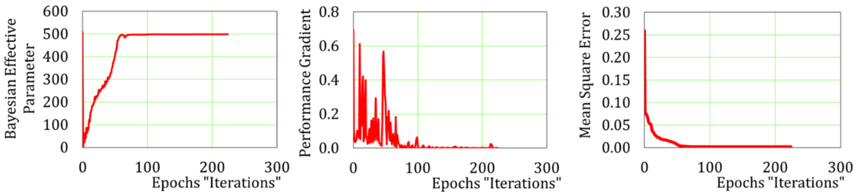
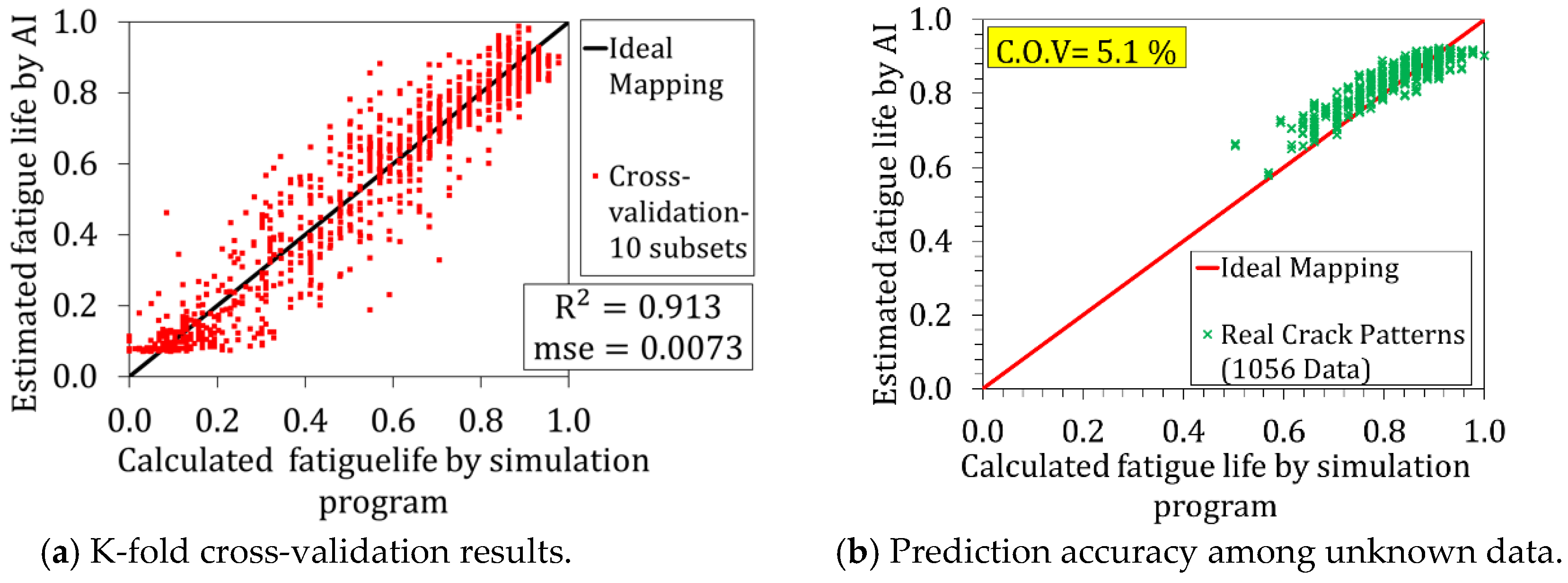
In this study, BRANN is used for training the RACP simulation results which are shown previously in Figure 7. The training parameters such as effective one of BRANN, performance gradient and mean square errors reach stable states as shown in Figure 15. If the training parameters for BRANN reach stable states, it typically means the solution is truly converged. In order to ensure that a generalized solution is achieved by Bayesian regularization technique, k-fold cross-validation is conducted [34,35], where the dataset (RACPs) is divided into 10 subsets. Each subset will be treated as a validation dataset, while the rest is used as a training dataset. Then the prediction accuracy is checked for the 10 validation subsets, where it resembles the total dataset. Figure 16a shows the results of the k-fold cross-validation, where the regression coefficient of prediction (R2) is 0.913 and the mean square errors’ (mse) value is 0.0073. The results demonstrate the generalization of the network, where it maps almost all the validation subsets with good accuracy.
Moreover, the authors decided to test the network with independent real crack patterns besides their mirror cases (1056 data) to check the robustness of the network to treat unknown data. The relation of the fatigue life by the multi-scale simulation and the one of the built ANN for the test dataset is shown in Figure 16b. The validation around the best-fit line is with 5.1% of the coefficient of variation of prediction (C.O.V).
5.7. Structural Mechanistic Expressions of ANN’s Weights
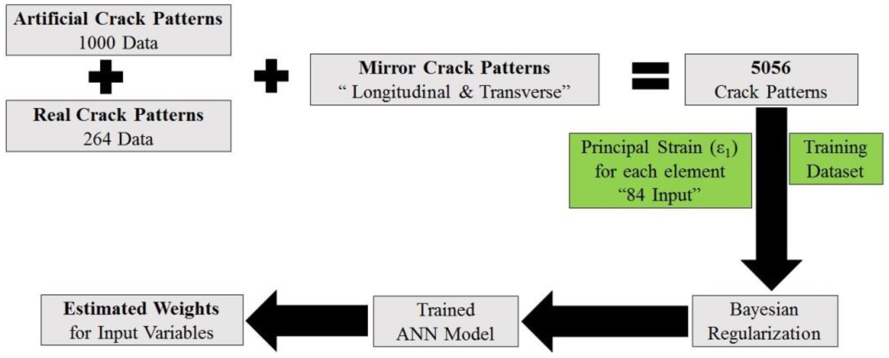
Generally, ANN is not a tool for achieving mechanistic principles but it may lead to some hints or foresight on the unknown or something uncertain. In this section, the authors try to utilize the internal weight of individual neuron to achieve a hazard map for the location of higher risk cracking at the bottom surface of the RC deck and validate with the structural knowledge and site observation as shown in Figure 17. The ANN model used in this section is the simplest structure (one hidden layer & one neuron). Only the cracks magnitude of the 84 elements of the bottom surface RC deck (see Figure 12) is taken into account to show the impact of the location of the cracks on the remaining fatigue life. The training dataset includes 1000 RACPs and 264 real crack patterns besides their mirror crack patterns in the transverse and the longitudinal directions (5056 crack patterns).
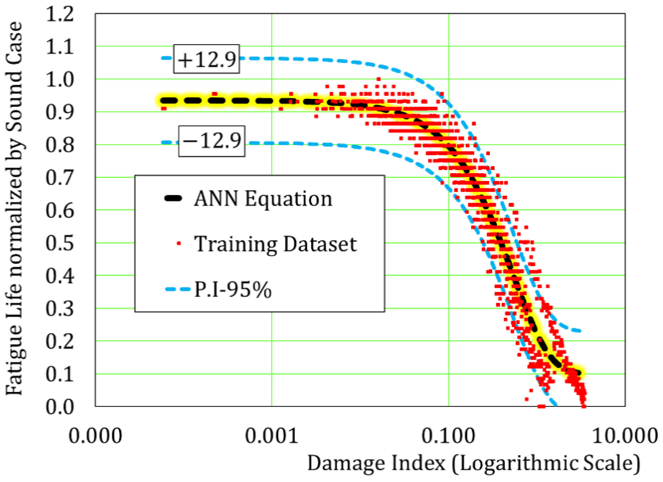
Bayesian regularization technique is used to prevent overtraining and to eliminate the need for lengthy cross-validations. Equation (8) shows the prediction correlation of the trained ANN model, where it is a function of the elements principal strains (84 elements). Figure 18 shows the relation of the damage index (see Equation (9)) and the normalized fatigue life, where the remaining fatigue life decreases by increasing in the damage index. The results show that the ANN maps the training dataset with a good accuracy, where the prediction interval has a value of 12.9%.
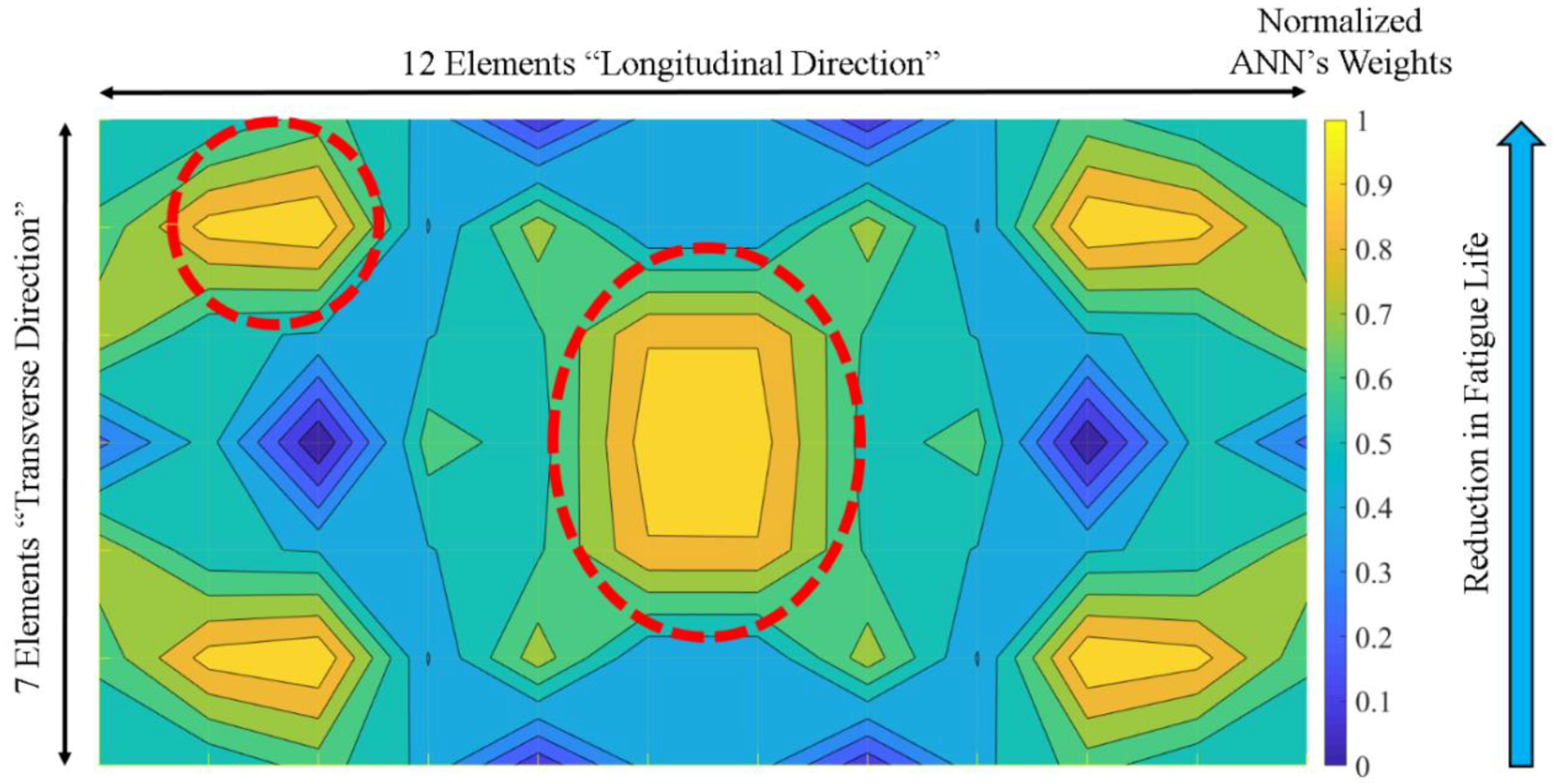
The weights of the individual neuron of the trained ANN can be described as the impact of the location of the crack on the remaining fatigue life. Figure 19 shows the weights distribution as contour lines, normalized between 0 & 1 of the discretized RC deck’s bottom surface (84 elements). The map shows the ANN model has learned the law of symmetry in both directions, where full symmetry is obtained. It is also found that the central zone and the corners of the RC deck are the locations of the higher risk cracking to reduce the fatigue life.
The locations of the highest risk cracking obtained from the estimated weights of the trained ANN model can be explained from a structural point of view. It is well known that the central zone of the RC deck has the maximum bending moment, while the corners have the maximum shear force based on the structural analysis of the slabs. Thus, the existence of pre-cracks at the central zone will stimulate the propagation of these cracks as flexural ones since the central zone is the location of the maximum bending moment. Therefore, deck’s stiffness is reduced and the fatigue life is shortened. The reduction of the stiffness may cause larger amplitude of repeated strains inside the structural concrete.
On the contrary, the existence of pre-cracks at the corners may initiate the harmful diagonal shear cracks. In fact, the previous research reported that the reason of the excessive deflection of the culvert’s top slabs was the occurrence of out-of-plane diagonal shear cracks at the corners [36]. Anyhow, bending actions hardly create cracks at the corners of the slabs. Then, if cracking is found in these areas, it should be understood as some sort of caution. The trained ANN could learn it appropriately with mechanical consistency.
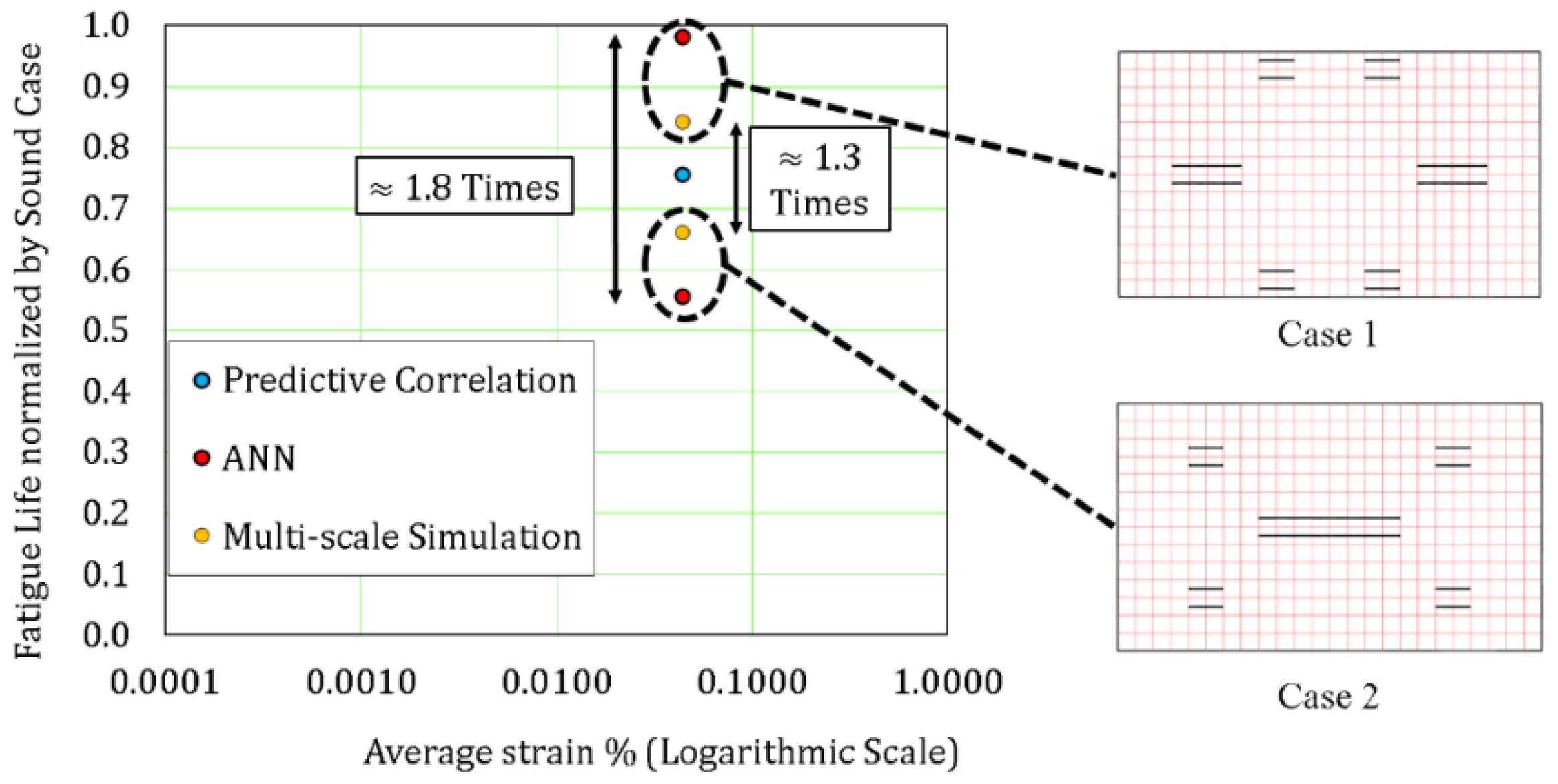
In order to demonstrate the role of AI for conducting a fair-detailed judgement for the deterioration magnitude of the RC deck regarding their crack patterns, a comparison has been done between the remaining fatigue lives of two investigated crack patterns, where they have exactly the same crack density but different cracks location, as shown in Figure 20. The difference between the remaining fatigue life obtained from the proposed ANN model and the multi-scale simulation program in this Section is 1.8 and 1.3 times respectively but the predictive correlation introduced in Section 4.3 cannot capture this difference and the remaining fatigue life is the same due to the lack of information of the average strain parameter.
where R.L is the remaining fatigue life, [S] is the input vector for the principal strains of the FEM elements (84 elements) and [W] is the trained ANN’s weight vector (known values).
R.L = 4.6 − 4.5 × Tanh (1.14 + [S]1×84 × [W]84×1)
Damage Index = [S]1×84 × [W]84×1
6. Conclusions
Two simplified fast-truck evaluation methods, which are numerically built on the basis of the integrated lifetime simulation system, are proposed for the quantitative damage assessment of RC decks in use of the crack inspection data. The statistical data processing with mechanics-based parameters is conducted and compared with the neural network learning with no scientific logic and the following conclusions are drawn.
- Two fast-truck quantitative assessment models for the magnitude of damages of in-situ RC bridge road decks in service were built based upon the training dataset created by numerical simulation as well as the real site inspection data. A quick and massive diagnosis, which is equivalent to the full 3D multi-scale simulation, is made possible.
- The statistical model is built on the basis of the mechanics-based parameter. Here, the conservative and safer-side assessment of the remaining fatigue life is practically made possible by avoiding the case where pre-cracking stops the preceding shear cracking.
- By examining the wide variety of crack orientation and their patterns over the bottom surfaces of RC decks, it is quantitatively proved that the geometrical patterns of cracking have much to do with the remaining fatigue life as well as crack width.
- By conduction k-fold cross-validation and testing the ANN model, the robustness and the generalization of the proposed ANN model are confirmed with the crack patterns observed at bridge construction site. Here, the numerically produced training dataset, which was offered by the multi-scale analysis, enables us to compensate the week spots of the training dataset.
- A hazard mapping to identify the high-risk location of cracking is created in use of the neuron’s weight and its sensitivity to the fatigue life. It is found that both RC deck’s central zone and their corners are the spots of caution. This map can be used as the guideline to train inspectors.
- It is proved that artificial intelligence is not just a tool for conducting predictive models but it can guide somehow to achieve physical expressions for a particular problem.
Author Contributions
E.F. and Y.T. built the univariate and artificial neural network (ANN) models based upon the leaning data which Y.T. and K.M. produced; Y.T. collected the inspection data of bridges at site; K.M. supervised over the analytical process; A.S. cross-validated the model’s reliability and supervised over the ANN; E.F. and K.M. wrote the paper.
Funding
This study was financially supported by Council for Science, Technology, and Innovation, “Cross-ministerial Strategic Innovation Promotion Program (SIP), Infrastructure Maintenance, Renovation, and Management” granted by JST.
Acknowledgments
The authors extend their appreciation to Prof. Yozo Fujino of Yokohama National University and The University of Tokyo, for his valuable advices and encouragement to bridge the multi-disciplines in engineering.
Conflicts of Interest
The authors declare no conflict of interest.
References
- NEXCO-Japan. Regarding Large-Scale Renewal and Large-Scale Repair on the Expressway Managed by Eastern, Central and West Japan Expressway Co., Ltd. 2014. Available online: https://www.c-nexco.co.jp/koushin/pdf/about.pdf (accessed on 17 May 2018).
- Japan Society of Civil Engineers. Standard Specifications for Concrete Structures—2017 “Maintenance”; JSCE Guidelines for Concrete; Japan Society of Civil Engineers: Tokyo, Japan, 2007. [Google Scholar]
- Maekawa, K.; Pimanmas, A.; Okamura, H. Nonlinear Mechanics of Reinforced Concrete; Spon Press: London, UK, 2003. [Google Scholar]
- Maekawa, K.; Ishida, T.; Kishi, T. Multi-Scale Modeling of Structural Concrete; Taylor & Francis: London, UK, 2009. [Google Scholar]
- Maekawa, K.; Toongoenthong, T.; Gebreyouhannes, E.; Kishi, T. Direct path-integral scheme for fatigue simulation of reinforced concrete in shear. J. Adv. Concr. Technol. 2006, 4, 159–177. [Google Scholar] [CrossRef]
- Fujiyama, C.; Tang, X.J.; Maekawa, K.; An, X. Pseudo-cracking approach to fatigue life assessment of RC bridge decks in service. J. Adv. Concr. Technol. 2013, 11, 7–21. [Google Scholar] [CrossRef]
- Tang, X.J.; Fujiyama, C.; An, X.H.; Maekawa, K. Pseudo cracking approach to fatigue life assessment of existing RC bridge decks based on crack inspection data. In Proceedings of the Thirteenth East Asia Pacific Conference on Structural Engineering and Construction (EASEC 13), Sapporo, Japan, 11–13 September 2013. [Google Scholar]
- Tanaka, Y.; Maekawa, K.; Maeshima, T.; Iwaki, I.; Nishida, T.; Shiotani, T. Data assimilation for fatigue life assessment of RC bridge decks coupled with hygro-mechanistic model and nondestructive inspection. J. Disaster Res. 2017, 12, 422–431. [Google Scholar] [CrossRef]
- Fathalla, E.; Tanaka, Y.; Maekawa, K. Parametrical study on fatigue life of road bridge decks with pseudo-cracking analysis. In Proceedings of the 8th Asia and Pacific Young Researchers and Graduates Symposium, Tokyo, Japan, 7–8 September 2017. [Google Scholar]
- Fathalla, E.; Tanaka, Y.; Maekawa, K. Remaining fatigue life assessment of in-service road bridge decks based upon artificial neural networks. Eng. Struct. 2018, 171, 602–616. [Google Scholar] [CrossRef]
- Fausett, L.V. Fundamentals of Neural Networks: Architectures, Algorithms, and Applications; Prentice-Hall: Englewood Cliffs, NJ, USA, 1994. [Google Scholar]
- M.I.T. Lincoln Laboratory. DARPA Neural Network Study; Defense Technical Information Center: Fort Belvoir, VA, USA, 1989. [Google Scholar]
- Grossberg, S. Studies of the Mind and Brain; Reidel Press: Drodrecht, The Netherlands, 1982. [Google Scholar]
- Hagan, M.T.; Demuth, H.B.; Beale, M.H.; Jesús, O.D. Neural Network Design; PWS Publishing: Boston, MA, USA, 1996. [Google Scholar]
- Japan Road Association. Specification for Highway Bridges—Part III Concrete Bridges; Japan Road Association: Tokyo, Japan, 2012. [Google Scholar]
- Matsui, S. Lifetime prediction of bridge. J. JSCE 1996, 30, 432–440. [Google Scholar]
- Maeshima, T.; Koda, Y.; Tsuchiya, S.; Iwaki, I. Influence of corrosion of rebars caused by chloride induced deterioration on fatigue resistance in RC road deck. J. JSCE E2 2014, 70, 208–225. [Google Scholar] [CrossRef]
- Kado, M.; Maeshima, T.; Koda, Y.; Nakano, S.; Fujiyama, C.; Iwaki, I. Study on a method of evaluating fatigue damage for RC bridge deck slab using long basis optical strand sensors. J. JSCE E2 2015, 71, 323–337. [Google Scholar] [CrossRef]
- Okada, K.; Okamura, H.; Sonoda, K.; Shimada, I. Cracking and fatigue behavior of bridge deck RC slabs. J. JSCE 1982, 321, 49–61. [Google Scholar] [CrossRef]
- Mizutani, T.; Nakamura, N.; Yamaguchi, T.; Tarumi, M.; Ando, Y. Signal processing for fast RC bridge slab damage detection by using UHF-band radar. In Proceedings of the 6th Asia Pacific Workshop on Structural Health Monitoring, Hobart, Australia, 7–9 December 2017. [Google Scholar]
- Kobayashi, Y.; Oda, K.; Shiotani, T. Three dimensional AE tomography with accurate source location technique. In Proceedings of the Structural Faults & Repair, London, UK, 8–10 July 2014. [Google Scholar]
- Nair, A.; Cai, C.S. Acoustic emission monitoring of bridges: Review and case studies. Eng. Struct. 2010, 32, 1704–1714. [Google Scholar] [CrossRef]
- Takeuchi, H.; Ozawa, I.; Yano, R.; Mitsuya, Y.; Dobashi, K.; Uesaka, M.; Tanaka, Y.; Takahashi, Y.; Kusano, J.; Yoshida, E.; et al. Quantification of transmission X-ray imaging capability of portable X-ray source in concrete bridge inspection. J. JSCE E2 2018, 74, 66–79. [Google Scholar] [CrossRef]
- Ikeda, Y.; Takamura, M.; Taketani, A.; Sunaga, H.; Otake, Y.; Suzuki, H.; Kumagai, M.; Oba, Y. Prospect for application of compact accelerator-based neutron source to neutron engineering diffraction. Nucl. Instrum. Methods Phys. Res. Sect. A 2016, 833, 61–67. [Google Scholar] [CrossRef]
- Tanaka, Y.; Kishi, T.; Maekawa, K. Experimental research on the structural mechanism of RC members containing artificial crack in shear. JSCE 2005, 802, 109–121. [Google Scholar] [CrossRef]
- Tanaka, Y.; Kishi, T.; Maekawa, K. Tied arch system and evaluation method of shear strength of RC members containing artificial crack or unbond zone. JSCE 2005, 788, 175–193. [Google Scholar]
- Niwa, J.; Yamada, K.; Yokozawa, K.; Okamura, H. Revaluation of the equation for shear strength of reinforced concrete beams without web reinforcement. J. JSCE 1986, 372, 65–84. [Google Scholar] [CrossRef]
- Murphy, K.P. Machine Learning: A Probabilistic Perspective; The MIT Press: Cambridge, MA, USA, 2012. [Google Scholar]
- Hagan, M.T.; Menhaj, M. Training feed-forward networks with the Marquardt algorithm. IEEE Trans. Neural Netw. 1994, 15, 989–993. [Google Scholar] [CrossRef] [PubMed]
- Rumelhart, D.; Hinton, G.; Williams, R. Learning representations by back-propagating errors. Nature 1986, 323, 533–536. [Google Scholar] [CrossRef]
- Burden, F.; Winkler, D. Bayesian Regularization of Neural Networks, in Artificial Neural Networks. Methods Mol. Biol. 2008, 458, 25–44. [Google Scholar] [PubMed]
- Foresee, F.D.; Hagan, M.T. Gauss-Newton approximation to Bayesian regularization. In Proceedings of the International Joint Conference on Neural Networks, Nagoya, Japan, 23–29 August 1997. [Google Scholar]
- MacKay, D.J.C. Bayesian Interpolation. Neural Comput. 1992, 4, 415–447. [Google Scholar] [CrossRef]
- Geisser, S. Predictive Inference; Chapman and Hall: New York, NY, USA, 1993. [Google Scholar]
- Picard, R.R.; Cook, R.D. Cross-Validation of Regression Models. J. Am. Stat. Assoc. 1984, 79, 575–583. [Google Scholar] [CrossRef]
- Maekawa, K.; Zhu, X.; Chijiwa, N.; Tanabe, S. Mechanism of long-term excessive deformation and delayed shear failure of underground RC box culverts. J. Adv. Concr. Technol. 2016, 14, 183–204. [Google Scholar] [CrossRef]
Figure 1.
Data assimilation technology.

Figure 2.
High cycle wheel-type traveling load and the target slab.

Figure 3.
Investigated real crack patterns.

Figure 4.
Cyclic passage of moving wheel type load versus live-load deflection at span center for the referential RC deck.
Figure 4.
Cyclic passage of moving wheel type load versus live-load deflection at span center for the referential RC deck.

Figure 5.
Cracks depth for sets 1 & 2 and pre-cracks stopping mechanism.

Figure 6.
Comparison of sets 1 & 2 regarding the remaining fatigue life.

Figure 7.
Relationship between the average strain and the fatigue life of real crack patterns and randomized artificial crack pattern program (RACPs).
Figure 7.
Relationship between the average strain and the fatigue life of real crack patterns and randomized artificial crack pattern program (RACPs).

Figure 8.
Strategy of the training dataset.

Figure 9.
Randomized artificial crack patterns scheme.

Figure 10.
Relationship between cracks density and the remaining fatigue life.

Figure 11.
Proposed correlation for the remaining fatigue life prediction by using cracks density parameter.
Figure 11.
Proposed correlation for the remaining fatigue life prediction by using cracks density parameter.

Figure 12.
Input and output variables in fatigue life oriented neural network for cases (3) & (4).

Figure 13.
Effect of traffic direction on remaining fatigue lives corresponding to crack patterns.

Figure 14.
Relationship between the fatigue life of “multiscale simulation program” & “ANN” for the training dataset.
Figure 14.
Relationship between the fatigue life of “multiscale simulation program” & “ANN” for the training dataset.

Figure 15.
Training parameters’ states during learning.

Figure 16.
K-fold cross-validation & ANN’s robustness among unknown data.

Figure 17.
Strategy for achieving hazard map for the locations of higher risk cracking.

Figure 18.
Relationship between damage index and the normalized remaining fatigue life.

Figure 19.
Contours of the cracks location impact on the remaining fatigue life.

Figure 20.
Comparison of the remaining fatigue life between two crack patterns of the same cracks density.
Figure 20.
Comparison of the remaining fatigue life between two crack patterns of the same cracks density.


Table 1.
Material properties of the referential target reinforced concrete (RC) slab.
| Material Type | Concrete | Steel Reinforcement | |
|---|---|---|---|
| Young’s Modulus | N/mm2 | 24,750 | 205,000 |
| Compressive Strength | N/mm2 | 30 | 295 |
| Tensile Strength | N/mm2 | 2.2 | 295 |
| Specific Weight | kN/m3 | 24 | 78 |
Table 2.
Four sets of input variables for choosing the best performance artificial neural networks (ANN) model.
Table 2.
Four sets of input variables for choosing the best performance artificial neural networks (ANN) model.
| ANN Input Variables | Variables for Each FEM Element | No. of Elements | Total Number of Variables | Cracks Direction |
|---|---|---|---|---|
| Case (1) | εxx, εyy, εxy | 336 | 1008 | Included “Indirectly” |
| Case (2) | ε1, θ (Equations (6) and (7)) | 336 | 672 | Included “Directly” |
| Case (3) | εxx, εyy, εxy | 84 | 252 | Included “Indirectly” |
| Case (4) | ε1, θ (Equations (6) and (7)) | 84 | 168 | Included “Directly” |
Table 3.
ANN’s structure.
| ANN Input Variables | Number of Hidden Layers | Number of Neurons |
|---|---|---|
| Case 1 | 1 | 1 |
| Case 2 | 1 | 1 |
| Case 3 | 1 | 2 |
| Case 4 | 1 | 2 |
| Case 5 Section 5.5 | 1 | 2 |
Table 4.
Two sets of input variables to show cracks direction significance.
| ANN Input Variables | Variables for Each FEM Element | No. of Elements | Total Number of Variables | Cracks Direction |
|---|---|---|---|---|
| Case (3) | εxx, εyy, εxy | 84 | 252 | Included “Indirectly” |
| Case (5) | ε1 | 84 | 84 | Not included |
© 2018 by the authors. Licensee MDPI, Basel, Switzerland. This article is an open access article distributed under the terms and conditions of the Creative Commons Attribution (CC BY) license (http://creativecommons.org/licenses/by/4.0/).
Share and Cite
MDPI and ACS Style
Fathalla, E.; Tanaka, Y.; Maekawa, K.; Sakurai, A. Quantitative Deterioration Assessment of Road Bridge Decks Based on Site Inspected Cracks. Appl. Sci. 2018, 8, 1197. https://doi.org/10.3390/app8071197
AMA Style
Fathalla E, Tanaka Y, Maekawa K, Sakurai A. Quantitative Deterioration Assessment of Road Bridge Decks Based on Site Inspected Cracks. Applied Sciences. 2018; 8(7):1197. https://doi.org/10.3390/app8071197
Chicago/Turabian StyleFathalla, Eissa, Yasushi Tanaka, Koichi Maekawa, and Akito Sakurai. 2018. "Quantitative Deterioration Assessment of Road Bridge Decks Based on Site Inspected Cracks" Applied Sciences 8, no. 7: 1197. https://doi.org/10.3390/app8071197
Note that from the first issue of 2016, this journal uses article numbers instead of page numbers. See further details here.