Integrated Adaptive Cruise Control with Weight Coefficient Self-Tuning Strategy

1
Automotive Electronics Center, Institute of Microelectronics of Chinese Academy of Sciences, Beijing 100029, China
2
University of Chinese Academy of Sciences, Beijing 100049, China
3
Kunshan Department, Institute of Microelectronics, Chinese Academy of Sciences, Kunshan 215347, China
*
Author to whom correspondence should be addressed.
Appl. Sci. 2018, 8(6), 978; https://doi.org/10.3390/app8060978
Submission received: 19 April 2018
/
Revised: 1 June 2018
/
Accepted: 1 June 2018
/
Published: 15 June 2018
Abstract
:This paper presents a novel multi-objective coordinated adaptive cruise control (ACC) algorithm based on a model predictive control (MPC) framework which can comprehensively address issues regarding longitudinal car-following performance, lateral stability, as well as vehicle safety. During the car-following, vehicle dynamics, illustrating the forces acting on the tire contact patches, are established. To simplify the tightly coupled dynamics system, a state-feedback based disturbance decoupling method is employed, by which longitudinal and lateral dynamics can be completely decoupled. Furthermore, the traditional MPC control with a constant weight matrix will probably not be able to solve time-varying multi-objective coordinated optimization issues, especially in transient scenarios. A weight coefficient self-tuning strategy is therefore suggested by which the weight coefficient for each sub-objective can be adjusted automatically with the change of traffic scenarios, accordingly improving the overall car-following performance. The simulations show that the control algorithm utilizing the suggested self-tuning strategy reaps significant benefits in terms of longitudinal car-following performance, while at the same time maintaining a small lateral stability error range.

1. Introduction
The adaptive cruise control (ACC) system is the commercial implementation of the advanced driver assistance system (ADAS) that can reduce drivers’ workload (e.g., taking over the longitudinal control task), and improve vehicle safety as well as traffic flow [1,2]. The designs of current commercial ACC systems mainly focus on tracking a desired speed or maintaining a desired safe distance from preceding vehicles in the same lane. Additionally, various studies have recently begun to explore additional objectives such as fuel economy, longitudinal ride comfort, lateral stability, and vehicular physical limitations [2,3,4,5,6]. As these mentioned objectives usually conflict with each other [5], coordinating them simultaneously still presents a lot of challenges for designers, especially under complicated and volatile traffic scenarios.
Ioannou et al. [7] pointed out that fuel consumption was much higher under conditions of large acceleration/deceleration, lane changing, as well as cut-in/cut-off. On this basis, Jonsson et al. [8] suggested reducing fuel consumption while decreasing tracking capability. With respect to the longitudinal ride comfort, the vehicle longitudinal acceleration and its derivative (jerk) are typically restrained [9]. To improve lateral stability, researchers typically employ a direct yaw-moment control (DYC) system [10,11]. Importantly, an emergency braking, road surface disturbance or a sudden strong side wind might result in vehicle deflection during the longitudinal car-following [11], and furthermore ACC and DYC are reversely interactive with each other under some traffic scenarios [12]. Zhang et al. [12] therefore present a curving ACC system that is coordinated with a DYC system and gives consideration to both the longitudinal car-following performance and lateral stability on curved roads. The developed control system provides significant benefits in weakening the impact of DYC on the longitudinal car-following performance while also improving the lateral stability. What is more, in order to achieve the multiple objectives mentioned above, it is natural to introduce a model predictive control (MPC) framework, whose advantages in ACC controllers have recently been proven [2,5,6].
However, the traditional model predictive control algorithm with a constant weight matrix will probably not be able to improve the overall performance in transient scenarios [13]. Zhao et al. [13] pointed out that the traditional model predictive control algorithm with a constant weight matrix cannot meet the improvement requirement in fuel economy and ride comfort, and accordingly proposed a real-time weight tuning strategy to solve time-varying multi-objective control problems, where the weight matrix can be adjusted with respect to different operating conditions. In addition, when the weight coefficient for each sub-objective is constant, it is easy to cause the distribution of solutions to be more concentrated, and accordingly it will be difficult to achieve the global optimum [14]. For instance, when the current traffic scenario is emergent and severe, the longitudinal tracking capability should be most important to avoid a rear-end collision, which indicates that the importance (namely weight coefficient) of such a sub-objective in the MPC cost function should be paid more attention to. Similarly, when the tire-road friction coefficient is small, or the road curvature is large, priority should be given to the lateral stability for driving safety consideration.
As the lateral stability of an automotive vehicle in a steering maneuver is critical to the overall safety [11], an integrated adaptive cruise control (IACC) model which takes the longitudinal inter-vehicle and lateral dynamics into consideration as a whole is suggested so as to achieve a maximization of the longitudinal car-following performance while guaranteeing the lateral stability. Furthermore, to solve the time-varying multi-objective coordinated optimization issues explained above, a weight coefficient self-tuning strategy is thus proposed, where the weight coefficient for each sub-objective can be adjusted automatically with the change of traffic scenarios.
The rest of this paper is organized as follows. Section 2 presents the modeling of an integrated car-following system. Section 3 quantifies performance indexes for IACC. Section 4 suggests the dynamic weight coefficient adjustment strategy as well as receding optimization control algorithm based on MPC. Simulations and analysis are discussed in Section 5. Lastly, conclusions are drawn in Section 6.
2. Modeling of Integrated Car-Following System
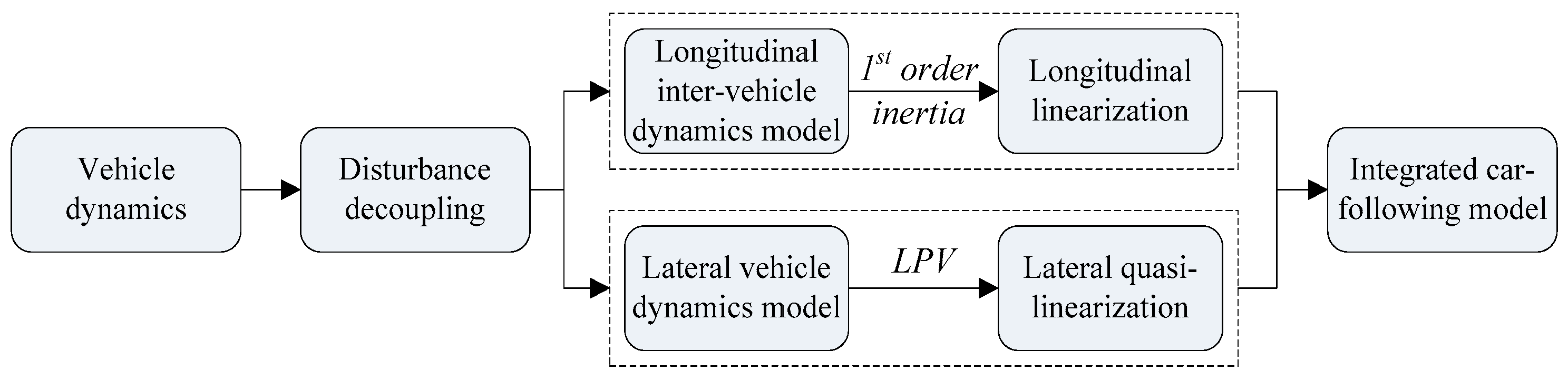
Section 2 is mainly organized as shown in Figure 1. During the car-following, vehicle dynamics, illustrating the forces acting on the tire contact patches, are established. To simplify the tightly coupled dynamics system, a state-feedback based disturbance decoupling method [15] is employed, by which longitudinal and lateral dynamics can be completely decoupled. After that, the longitudinal inter-vehicle model and lateral dynamics model are derived, as well as linearized, respectively. Finally, the integrated car-following state space model based on the MPC framework is designed.
2.1. Vehicle Dynamics
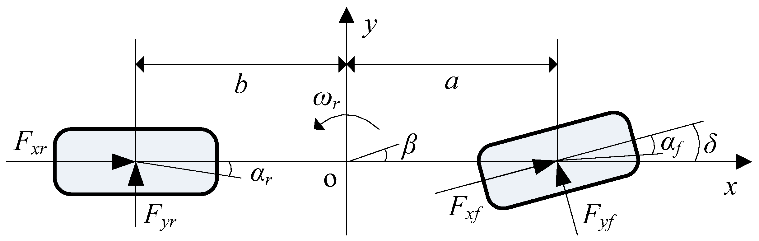
As illustrated in Figure 2, the longitudinal (x-direction), lateral (y-direction) and yaw dynamics during the car-following can be described as the equations below.
where and are longitudinal tire contact patch forces, while and are lateral ones. and are the moment of inertia of the front and rear tires, whose rolling radius is . is the longitudinal speed, is the lateral speed, and is the yaw rate. is the mass of the vehicle, is the gravitational acceleration, is the rolling resistance coefficient, is the road wheel angle of the front and is the road slope. is the drag coefficient, is the air density, and is the frontal area of the vehicle. and are the distances from the center of the mass (CM) of the vehicle to the front and rear axles respectively, is the yaw inertia, and is the desired yaw moment.
Now the assumptions below are made to simplify Equation (1):
- road wheel angle is tiny so that .
- road slope is assumed to be neglected.
Then we obtain
where , .
2.2. Disturbance Decoupling
Furthermore, the lateral forces and are assumed to linearly vary with the tire slip angles and respectively [16].
where and are the cornering stiffness of the front and rear tires respectively.
Besides, the tire slip angles associated with each wheel can be related to the body side-slip angle , road wheel angle and the yaw rate by the relationships below.
Integrating Equations (3)–(5), we obtain a 2-DOF vehicle model, which can be used for a lateral stability controller design.
Regarding Equation (2), there is a time-varying item: , which changes with the road wheel angle , longitudinal speed , lateral speed and the yaw rate . The idea of disturbance decoupling, as shown in Figure 3, is trying to find a state-feedback so as to construct a closed-loop system [15].
Then the decoupled longitudinal dynamics is rewritten as
2.3. Longitudinal Dynamics Model
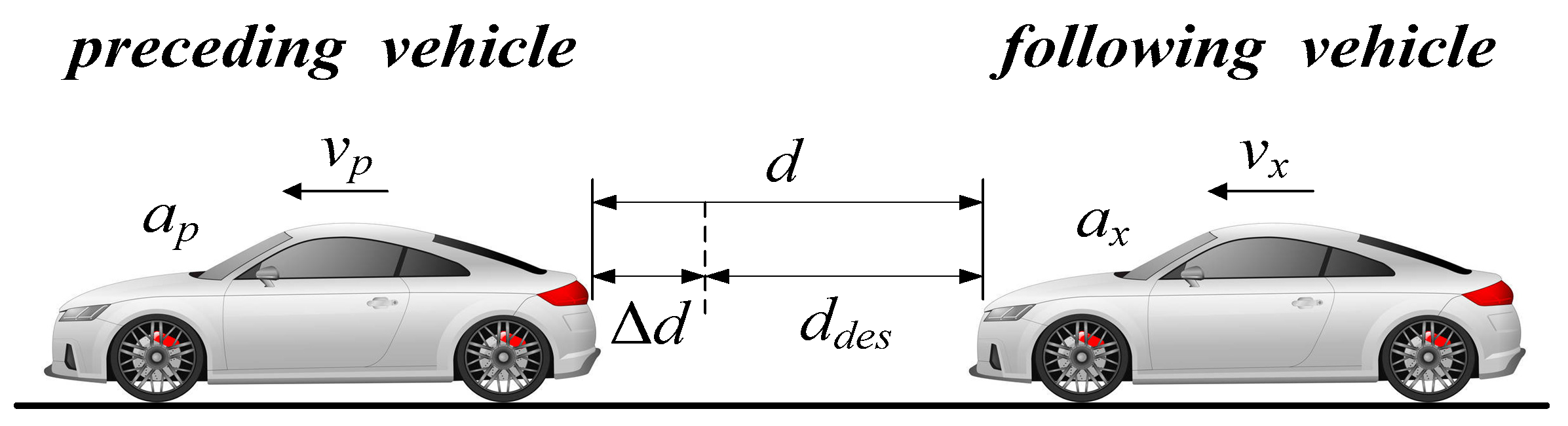
As illustrated in Figure 4, three state variables are defined: the distance error , speed error and derivative of the longitudinal acceleration (jerk for short) j, which can be described as
where is the actual inter-vehicle distance, is the desired inter-vehicle distance, , and , are the longitudinal speed/acceleration of the preceding vehicle and the following vehicle respectively.
With respect to , the constant time headway (CTH) spacing policy [17] is employed, which changes linearly with the speed of the following vehicle.
where is the nominal time headway and is the zero-speed clearance.
In addition, the decoupled longitudinal dynamics of the vehicle (see Figure 3) is still nonlinear, mainly due to the nonlinearity of the engine torque maps, time-varying gear position, as well as aerodynamic drag force [18]. In order to linearize the longitudinal dynamics of the vehicle, we introduce a first-order inertial system [5], whose transfer function is described as
where is the system gain and is the time constant.
Integrating Equations (8)–(10), a four state space model for longitudinal car-following dynamics can be formulated as
where , , , k represents the kth sampling point, , and are the state matrices, mathematically expressed as
2.4. Lateral Dynamics Model
As shown in Equation (6), a 2-DOF model is always used for the lateral stability controller design [12,19]. Additionally, the matrix representation of Equation (6) is described as
where , , , , and are the state matrices, mathematically expressed as
Unlike the longitudinal dynamics model, the lateral dynamics model, whose state matrices change with the longitudinal speed , is time-varying. This means that the discretization of the state matrices should be carried out in every control cycle, with (the length of the predictive horizon) times increased on this basis if the receding horizon control (e.g., MPC) method is employed. Additionally, the main problem this causes is that the system’s real-time performance will be greatly worsened. To reduce the considerable computational burden, a linear parameter-varying (LPV) method [20] is applied, changing the nonlinear model into a linear parameter-varying one.
Firstly, the state matrix can be described as
where , , .
Secondly, two boundary vectors can be obtained because and achieve maximum / minimum values at the same time.
Then, the local linearization of Equation (13) in the boundaries can be expressed as
Thirdly, employing the zero-order hold (ZOH) method [5] with a sample time , the discretization of the state matrices in the boundaries can be expressed as
Finally, a two state space model for the lateral dynamics can be formulated as
where , , , , , , is weight coefficient, and .
During the MPC control process, the discretization of the state matrices, shown as Equation (16), is just carried out once. Additionally, in each control cycle, only the weight coefficient needs to be adjusted. Therefore, the LPV method has its merits in solving the problem earlier mentioned.
2.5. Integrated Car-Following Model
Via the integration of the longitudinal dynamics model (refer to Equation (11)) and lateral dynamics model (refer to Equation (17)), the IACC control plant model is built as
where , , , , , and are the state matrices, mathematically expressed as
3. Quantification of Performance Indexes
3.1. Cost Function for Longitudinal Car-Following Performance
It is accepted that the longitudinal car-following performance is usually evaluated via tracking errors: and . However, the strong convergence of tracking errors will result in a frequent acceleration or deceleration, which might weaken the lateral stability and also reduce the longitudinal ride comfort or fuel economy, while the poor convergence will also cause a great amount of problems such as frequent cut-in, unsatisfied driver response, or even rear-end collision. Thus, the longitudinal performance indexes are designed to achieve:
- During the steady car-following scenario, the tracking errors should converge to tiny values;
- If the preceding vehicle accelerates, the tracking errors should be in a driver-permissible tracking error range to reduce frequent cut-in or driver intervention, and while it decelerates, rear-end collision must be avoided;
- As the fuel consumption increases with the absolute increase of the vehicle acceleration [7], the fuel economy can be improved indirectly via penalizing acceleration;
- To promote longitudinal ride comfort, the longitudinal jerk should be decreased as much as possible [5];
- The level of longitudinal acceleration should be restrained to some extent to guarantee sufficient lateral stability [12].
Accordingly, employing a 2-norm for tracking errors, actual acceleration, jerk and desired acceleration, the longitudinal cost function is built as
where , , , and are the corresponding weight coefficients.
3.2. Cost Function for Lateral Stability
Generally, the direct yaw control (DYC) is introduced to improve the vehicle lateral stability which is critical to vehicle safety [11,12]. The purpose of DYC is to make the yaw rate error and side-slip angle error convergent to zero by means of adding an external yaw moment. However, the yaw moment is always generated from a differential braking, which will weaken the longitudinal tracking capability. Thus, the yaw rate error, side-slip angle error, as well as desired yaw moment should be penalized simultaneously.
Similarly, the lateral cost function is built as
where , and are the corresponding weight coefficients. , , , is the nominal vehicle lateral dynamics response [12].
3.3. Rear-End Safety
To avoid rear-end collisions, an inequality for rear-end safety is specified as
where is the actual inter-vehicle distance, is the safe inter-vehicle distance, is the critical minimum safe distance, and is the time-to-collision (TTC) value [5].
The constraint, shown as Equation (21), should be considered as a hard constraint, owing to the fact that a rear-end collision cannot be tolerated at all.
3.4. Adhesion Workload
As the longitudinal tracking capability, along with the lateral stability, is closely related to road adhesion, the adhesion workload is defined as
where is the maximum road adhesion coefficient and is the lateral acceleration. This further indicates that dangerous situations such as drift will occur if Equation (22) is violated. Thus, Equation (22) should also be considered as a hard constraint.
3.5. I/O Constraints
In view of vehicular physical limitations as well as the driver-permissible tracking error range, the minimum/maximum values of the control commands and state variables are constrained as follows.
3.6. Predictive Expression of Cost Function
To guarantee lateral stability, the differential braking which is used for generating the direct yaw moment, gives rise to the longitudinal deceleration, accordingly weakening the longitudinal car-following performance, while the over-pursuit for tracking capability would affect the lateral stability, which is extremely crucial to vehicle safety. Thus, the longitudinal tracking capability as well as lateral stability control should be coordinated simultaneously.
Integrating Equations (19) and (20), the p-steps predictive expression of the cost function is built as
where is the reference trajectory, and are the diagonal weight matrices, are the desired input values to be optimized.
4. Predictive Control Algorithm for IACC
4.1. Addressing Computing Infeasibility
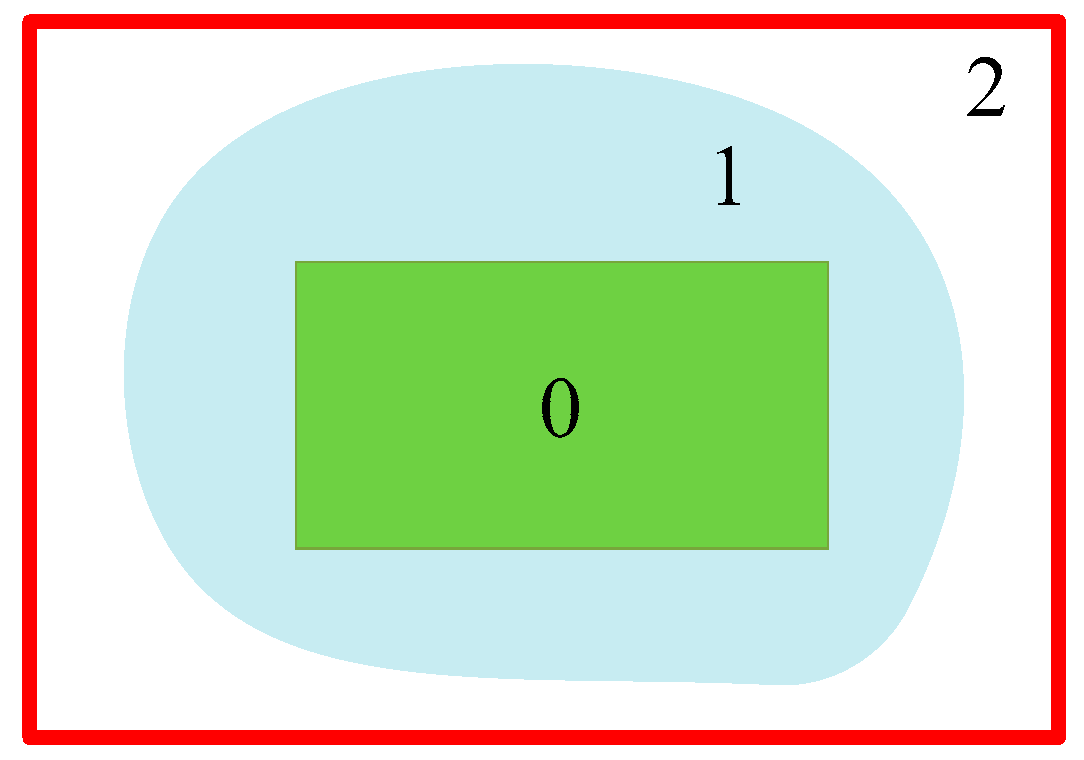
During the process of the receding horizon control, a key issue is the problem of computing infeasibility. There will be no optimal solution in case constraints, shown as Equations (21)–(23), are not satisfied. To avoid such issues, a constraint softening method, as illustrated in Figure 5, is employed to relax the hard I/O constraints [5,21].
As mentioned above, Equations (21) and (22) are so strict that they cannot be softened. Therefore, we just soften Equation (23) with a slack variable vector, and the corresponding soft constraint is expressed as
where , , , , are the corresponding slack variables, , and , , , , , , , , are the corresponding slack coefficients.
Moreover, when the boundaries of the hard constraints are not exceeded, the slack variables equal 0. Otherwise, the slack variables will increase automatically so as to guarantee the existence of a solution.
4.2. Multi-Objective Weights Self-Turning Strategy
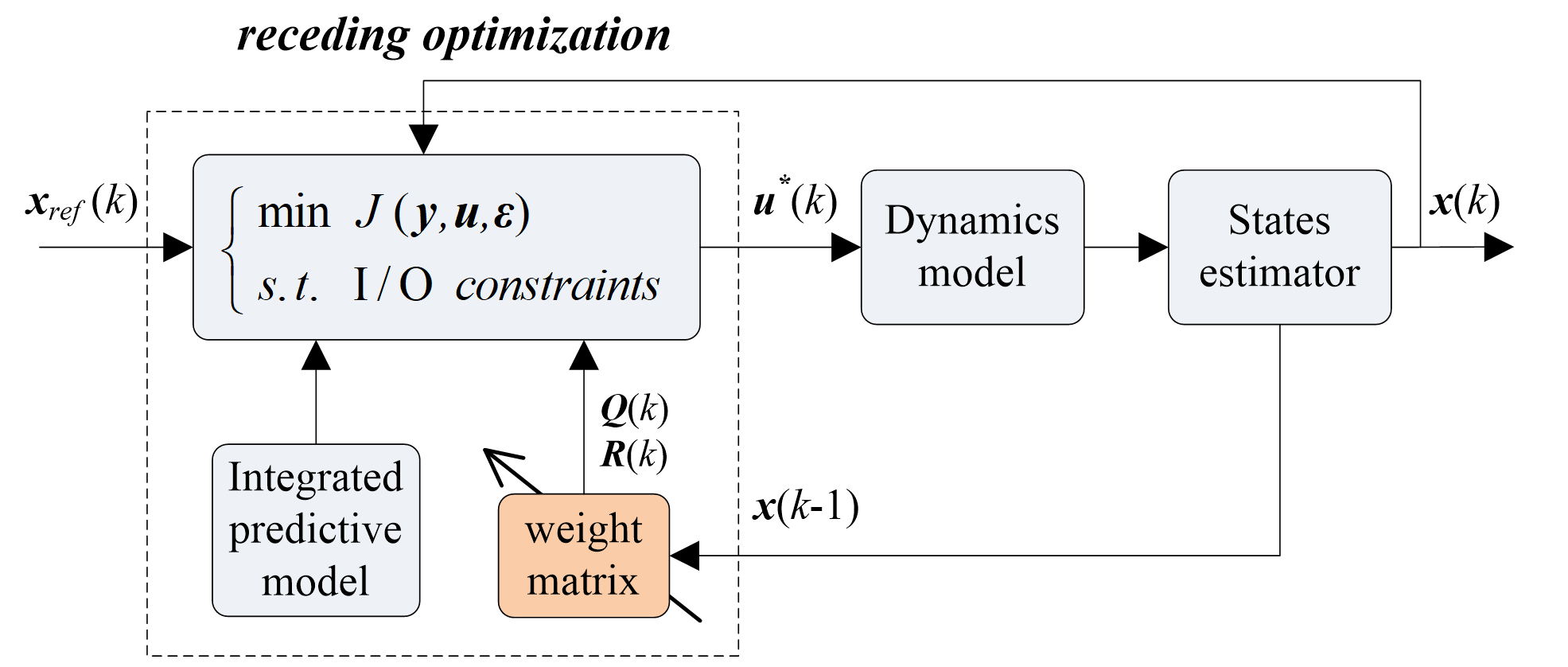
Regarding the multi-objective model predictive control algorithm, the value of the weight coefficient indicates the importance of the corresponding sub-objective. As previously mentioned, the traditional MPC control with a constant weight matrix (refer to Equation (24)) has inadequate adaptabilities against some transient traffic scenarios in particular. In addition, sub-objectives commonly conflict with each other. To increase the weight coefficient of one sub-objective will probably weaken the performance of others, which might cause the overall performance to be sub-optimal and sometimes even worsen the control quality. This indeed challenges the design of the ACC system especially, with regards to taking the complicated and volatile traffic scenarios into account.
To this end, it is worthwhile and also necessary to attempt to dynamically adjust the weight matrix with the change of traffic scenarios, as shown in Figure 6. For instance, when the road adhesion is poor or road curvature is large, the vehicle lateral stability should be paid more attention to in view of driving safety; accordingly, the corresponding weight coefficients will be larger than ever before. When the lateral stability is well-satisfied, priority should be given to the longitudinal tracking capability.
As the variance reflects the deviation degree of the random variable from the mathematical expectation, it can reflect the fluctuation of the variable more accurately than the mean.
The variance of each sub-objective is defined as
where is the variance of the corresponding sub-objective, such as .
The ratio of the sub-objective variance in the current cycle to that in last cycle is regarded as a tunable factor to adjust in correspondence with the weight coefficient. As a consequence, the weight coefficient self-tuning strategy is suggested as
where is the adjustment factor of the weight coefficient of the corresponding sub-objective, together with are the design parameters, and is the tuned weight coefficient for the cost function optimization in the next receding horizon.
4.3. Final Expression of Predictive Control Algorithm
In order to prevent the slack variables from increasing toward infinity, an additional quadratic term of slack variables is defined to penalize the violation of hard constraints so that it will be possible to make a balance between computing feasibility and the relaxation of constraints. The cost function in the finite predictive horizon, shown as Equation (24), is rewritten as
where is the slack variable vector, and is the penalized matrix.
Finally, the predictive optimization problem is to minimize the cost function Equation (28) subject to I/O constraints Equations (21), (22) and (25), which is eventually equivalent to solving Equation (29), as follows.
5. Simulations and Analysis
To validate and evaluate the improved performance of the proposed IACC controller with the weight coefficient self-tuning strategy, several numerical comparative simulations are conducted utilizing Matlab/Simulink and Carsim. The main parameters of the IACC controller are shown in Table 1.
The test scenario is supposed to be that the preceding vehicle, with an initial speed of 30 m/s, slows into the curve road with an emergent deceleration of −4.0 m/s2, then maintains a speed of 10 m/s for 15 s, and afterwards speeds up with an acceleration of 1.5 m/s2 to drive away, provided that the radius of the curve road is 350 m and that the tire-road friction coefficient is 0.8. What is more, the MPC based integrated control algorithm with tunable weight coefficients is simply called MPC-TW for short, while MPC-CW is short for the comparative one with constant weight coefficients.
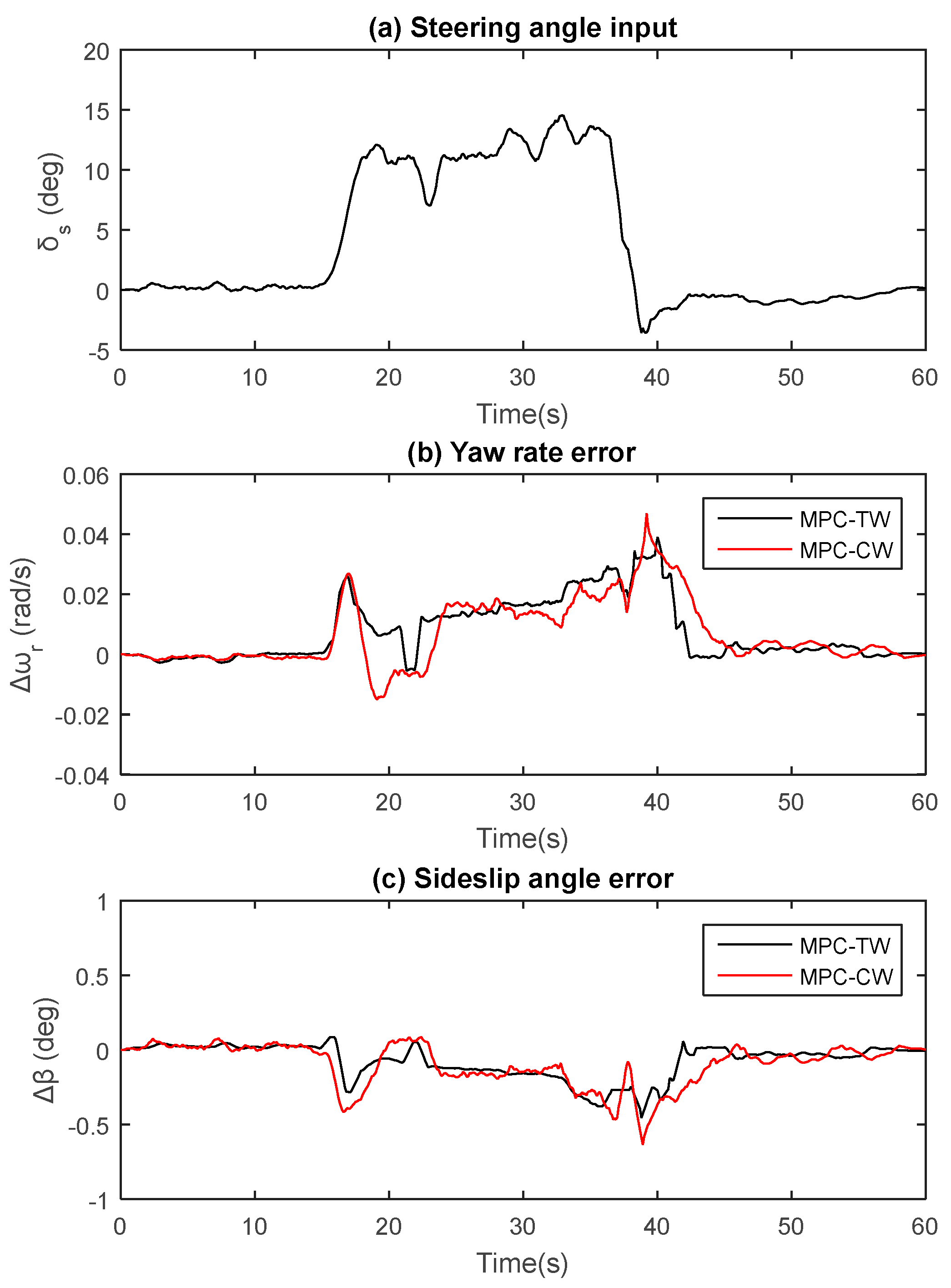
During the steering maneuver, priority should be given to lateral stability for driving safety consideration. Lateral stability (maintaining a small lateral stability error range) should be guaranteed for both MPC-TW and MPC-CW. As shown in Figure 7, both control methods can achieve a better performance in lateral stability.
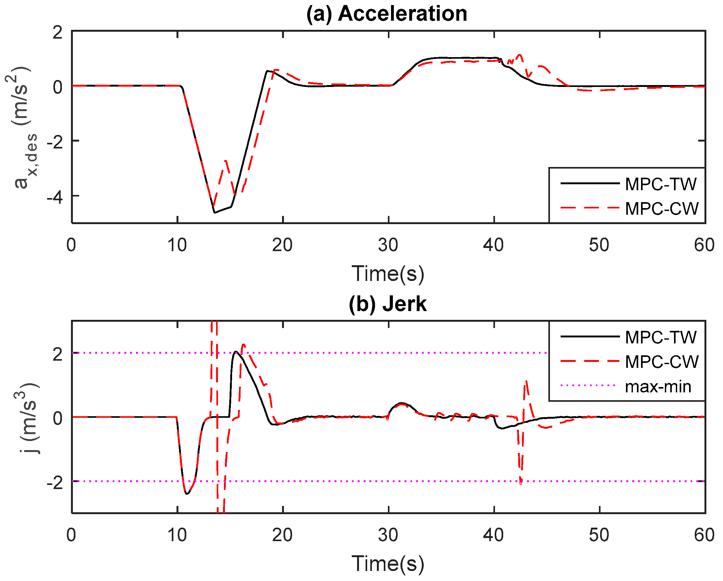
Figure 8, Figure 9 and Figure 10 show the longitudinal tracking response of speed, distance, acceleration and jerk, respectively. From Figure 8 and Figure 9, one can see that the MPC-CW cannot provide a substantial braking force in time when the preceding vehicle decelerates emergently at 10 s, and accordingly the inter-vehicle distance becomes shorter than that of MPC-TW. As shown in Figure 10, the MPC-TW can take an immediate brake as a result of tunable weights and also avoid overshooting to some extent, accordingly improving the longitudinal ride comfort. Furthermore, during the steering maneuver, the tracking capability of MPC-CW (from 30 s or so in Figure 8 and Figure 9) is somewhat sacrificed due to the extra brake pressure generated from the direct yaw moment. However, MPC-TW is able to weaken the impact of DYC applied to the longitudinal car-following performance by automatically tuning the weights of , and (see Figure 11), while maintaining a small lateral stability error range (see Figure 7). Moreover, from Figure 9, one can see that the introduction of a slack variable vector into the hard constraints (refer to Equation (23)) is able to satisfy the upper/lower boundary of inequality by increasing the corresponding slack variable when the boundary exceeds, shown as Equation (25), accordingly avoiding computing infeasibility.
Figure 11 shows the adjustment factor of the weight coefficient based on the self-tuning strategy suggested as Equation (27). Under the emergent scenario (from 10 s to 20 s or so), the weight of the desired acceleration, as well as the speed error, decreases because the corresponding adjustment factor shifts to less than 1, which indicates that the penalty for in the cost function becomes weakened, accordingly achieving a substantial braking force (see Figure 10) and also maintaining a better tracking capability (see Figure 8 and Figure 9).
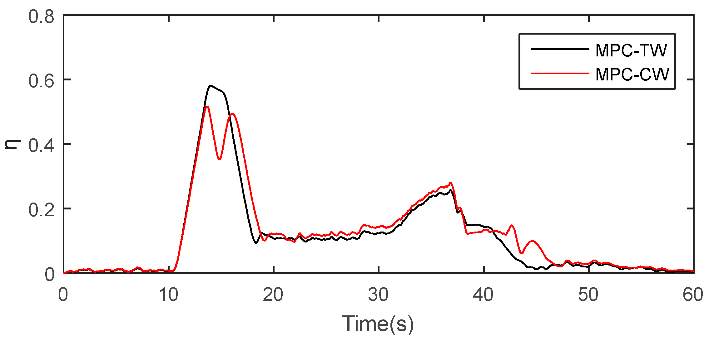
Additionally, a small adhesion workload means that the tires are far from the adhesion limit and that the vehicle still has great capacity for acceleration/deceleration and lateral stability [12]. As shown in Figure 12, the peak values for MPC-TW and MPC-CW are about 59% and 52%, respectively, accordingly guaranteeing another hard constraint, shown as Equation (22). Dangerous situations, such as spin or drift, always happen when the adhesion workload tends to its peak [12]. Although the proposed model improves the longitudinal tracking capability and lateral stability, it therefore clearly reduces vehicle safety. That is to say, under the transient scenarios, the pursuit for the longitudinal tracking capability as well as lateral stability should be sought under the premise of sufficient road adhesion capacity. Additionally, this means that the designing of an upper/lower boundary of the adjustment factor, shown as Equation (27), is in relation to the adhesion workload.
6. Conclusions
An IACC control plant model with a weight coefficient self-tuning strategy is suggested so as to achieve the maximization of the longitudinal car-following performance while guaranteeing lateral stability. The main conclusions drawn are as follows.
- (i)
- During the car-following, lateral stability should be given priority and can be well-guaranteed while satisfying a driver-permissible tracking range because input constraints, namely the longitudinal acceleration level, in the suggested IACC control algorithm, can be limited to a specific range.
- (ii)
- Compared with the traditional MPC control with a constant weight matrix, the weight coefficient self-tuning strategy can hopefully solve time-varying multi-objective coordinated optimization issues, where the weight coefficient for each sub-objective can be adjusted automatically with the change of traffic scenarios, thus improving the overall car-following performance.
- (iii)
- In addition, during the steering maneuver, MPC-TW is able to weaken the impact of DYC applied to the longitudinal tracking capability by automatically tuning the weight coefficients of the sub-objectives, while maintaining a small lateral stability error range.
Author Contributions
D.C. and Q.L. conceived and designed the experiments; J.Z. performed the experiments; J.Z. analyzed the data; S.L. from Tsinghua University contributed analysis tools; J.Z. wrote the paper.
Acknowledgments
The authors would like to thank all anonymous reviewers for their constructive comments and helpful suggestions on this research work. Meanwhile, the authors would like to thank financial support of STS Plan of Chinese Academy Science (No.: KFJ-STS-ZDTP-045).
Conflicts of Interest
The authors declare no conflicts of interest.
References
- Filho, C.; Terra, M.; Wolf, D. Safe optimization of highway traffic with robust model predictive control-based cooperative adaptive cruise control. IEEE Trans. Intell. Transp. Syst. 2017, 18, 3193–3203. [Google Scholar] [CrossRef]
- Dang, R.; Wang, J.; Li, S.; Li, K. Coordinated adaptive cruise control system with lane-change assistance. IEEE Trans. Intell. Transp. Syst. 2015, 16, 2373–2383. [Google Scholar] [CrossRef]
- Li, K.; Chen, T.; Luo, Y.; Wang, J. Intelligent environment-friendly vehicles: Concept and case studies. IEEE Trans. Intell. Transp. Syst. 2012, 13, 318–328. [Google Scholar] [CrossRef]
- Xiao, L.; Gao, F. A comprehensive review of the development of adaptive cruise control systems. Veh. Syst. Dyn. 2010, 48, 1167–1192. [Google Scholar] [CrossRef]
- Li, S.; Li, K.; Rajamani, R.; Wang, J. Model predictive multi-objective vehicular adaptive cruise control. IEEE Trans. Control Syst. Technol. 2011, 19, 556–566. [Google Scholar] [CrossRef]
- Li, S.; Jia, Z.; Li, K.; Cheng, B. Fast online computation of a model predictive controller and its application to fuel economy-oriented adaptive cruise control. IEEE Trans. Intell. Transp. Syst. 2015, 16, 1199–1209. [Google Scholar] [CrossRef]
- Ioannou, P.A.; Stefanovic, M. Evaluation of ACC vehicles in mixed traffic: Lane change effects and sensitivity analysis. IEEE Trans. Intell. Transp. Syst. 2005, 6, 79–89. [Google Scholar] [CrossRef]
- Jonsson, J. Fuel Optimized Predictive Following in Low Speed Conditions. Master’s Thesis, Department of Electrical Engineering, Linköping University, Linköping, Sweden, 2003. [Google Scholar]
- Ioannou, P.; Xu, Z. Throttle and brake control systems for automatic vehicle following. IVHS J. 1994, 1, 345–377. [Google Scholar] [CrossRef]
- Pi, D.W.; Chen, N.; Zhang, B.; Zhong, G.H. Enhancements in vehicle stability with yaw moment control via differential braking. In Proceedings of the 2009 IEEE Vehicular Electronics and Safety, Pune, India, 11–12 November 2010; pp. 136–140. [Google Scholar]
- Anwar, S. Generalized predictive control of yaw dynamics of a hybrid brake-by-wire equipped vehicle. Mechatronics 2005, 15, 1089–1108. [Google Scholar] [CrossRef]
- Zhang, D.; Li, K.; Wang, J. A curving ACC system with coordination control of longitudinal car-following and lateral stability. Veh. Syst. Dyn. 2012, 50, 1085–1102. [Google Scholar] [CrossRef]
- Zhao, R.C.; Wong, P.K.; Xie, Z.C.; Zhao, J. Real-time weighted multi-objective model predictive controller for adaptive cruise control systems. Int. J. Automot. Technol. 2017, 18, 279–292. [Google Scholar] [CrossRef]
- Zheng, D.; Gen, M.; Cheng, R. Multiobjective optimization using genetic algorithms. Eng. Valuat. Cost Anal. 1999, 2, 303–310. [Google Scholar]
- Bin, Y.; Li, K.; Hiroshi, U. Nonlinear disturbance decoupling control of heavy-duty truck stop and go cruise system. Veh. Syst. Dyn. 2009, 47, 29–55. [Google Scholar]
- Kiencke, U.; Nielsen, L. Automotive Control Systems: For Engine, Driveline, and Vehicle. Sens. Rev. 2005, 11, 1828. [Google Scholar]
- Yi, K.; Kwon, Y. Vehicle-to-vehicle distance and speed control using an electronic-vacuum booster. JSAE Rev. 2001, 22, 403–412. [Google Scholar] [CrossRef]
- Rajamani, R. Vehicles Dynamics and Control; Springer: New York, NY, USA, 2006. [Google Scholar]
- Cho, W.; Yoon, J.; Kim, J.; Hur, J.; Yi, K. An investigation into unified chassis control scheme for optimised vehicle stability and manoeuvrability. Veh. Syst. Dyn. 2008, 46, 87–105. [Google Scholar] [CrossRef]
- Apkarian, P.; Gahinet, P.; Becker, G. Self-scheduled H∞ control of linear parameter-varying systems: A design example. Automatica 1995, 31, 1251–1261. [Google Scholar] [CrossRef]
- Maciejowski, J. Predictive Control with Constraints; Pearson Education: Harlow, UK, 2002. [Google Scholar]
Figure 1.
Flow chart of integrated car-following decoupling and linearization; LPV: linear parameter-varying.
Figure 1.
Flow chart of integrated car-following decoupling and linearization; LPV: linear parameter-varying.

Figure 2.
Schematic representing vehicle dynamics.

Figure 3.
Disturbance decoupling via a state-feedback.
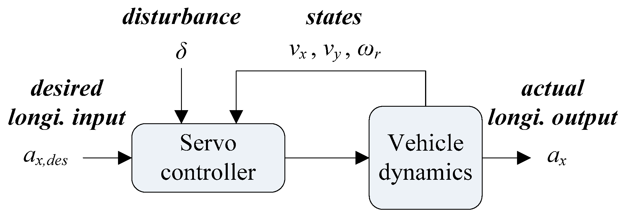
Figure 4.
Sketch of longitudinal car-following.

Figure 5.
Sketch of system IO constraints. 0—steady driving zone, 1—computing feasible sets, and 2—collision boundary.
Figure 5.
Sketch of system IO constraints. 0—steady driving zone, 1—computing feasible sets, and 2—collision boundary.

Figure 6.
Schematic diagram of IACC control algorithm with tunable weight coefficients.
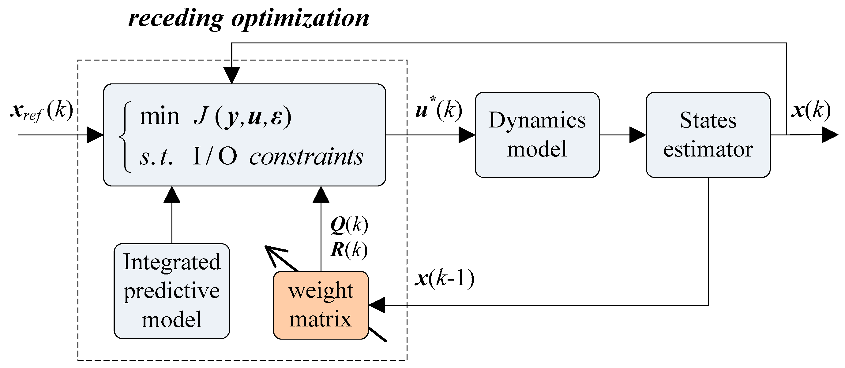
Figure 7.
Yaw rate error and side-slip angle error.

Figure 8.
Speed.
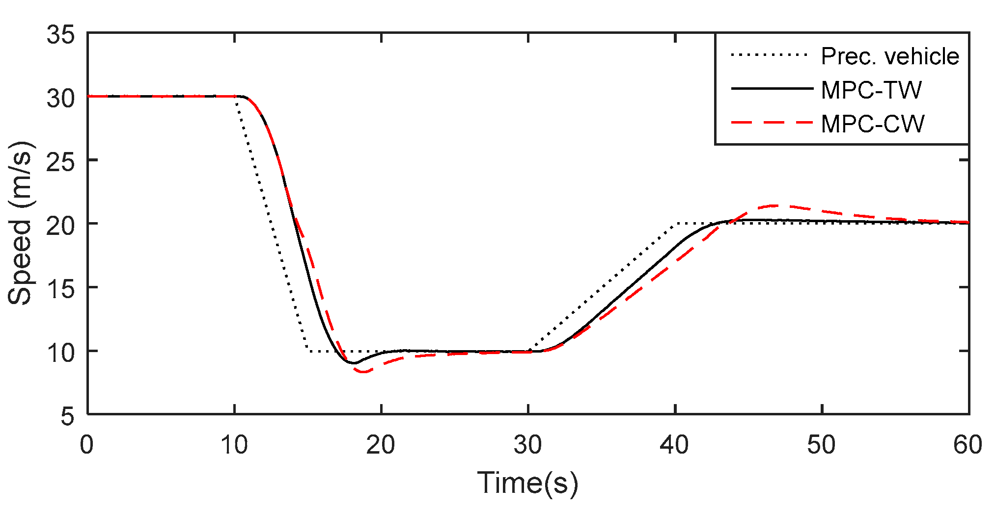
Figure 9.
Actual inter-vehicle distance and distance error.
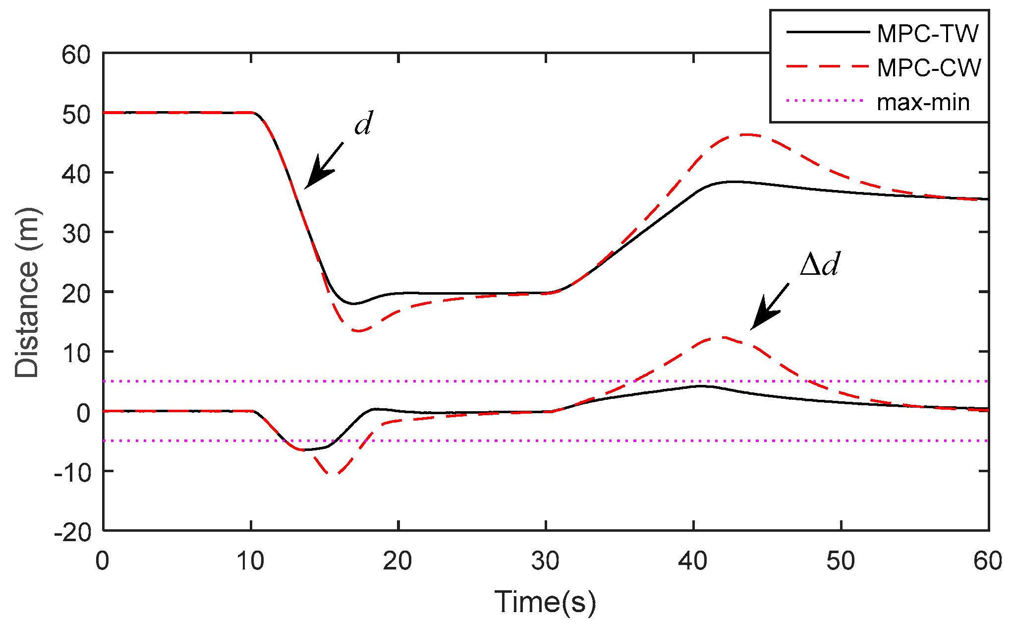
Figure 10.
Acceleration and jerk.

Figure 11.
Adjustment factor for weight coefficient.
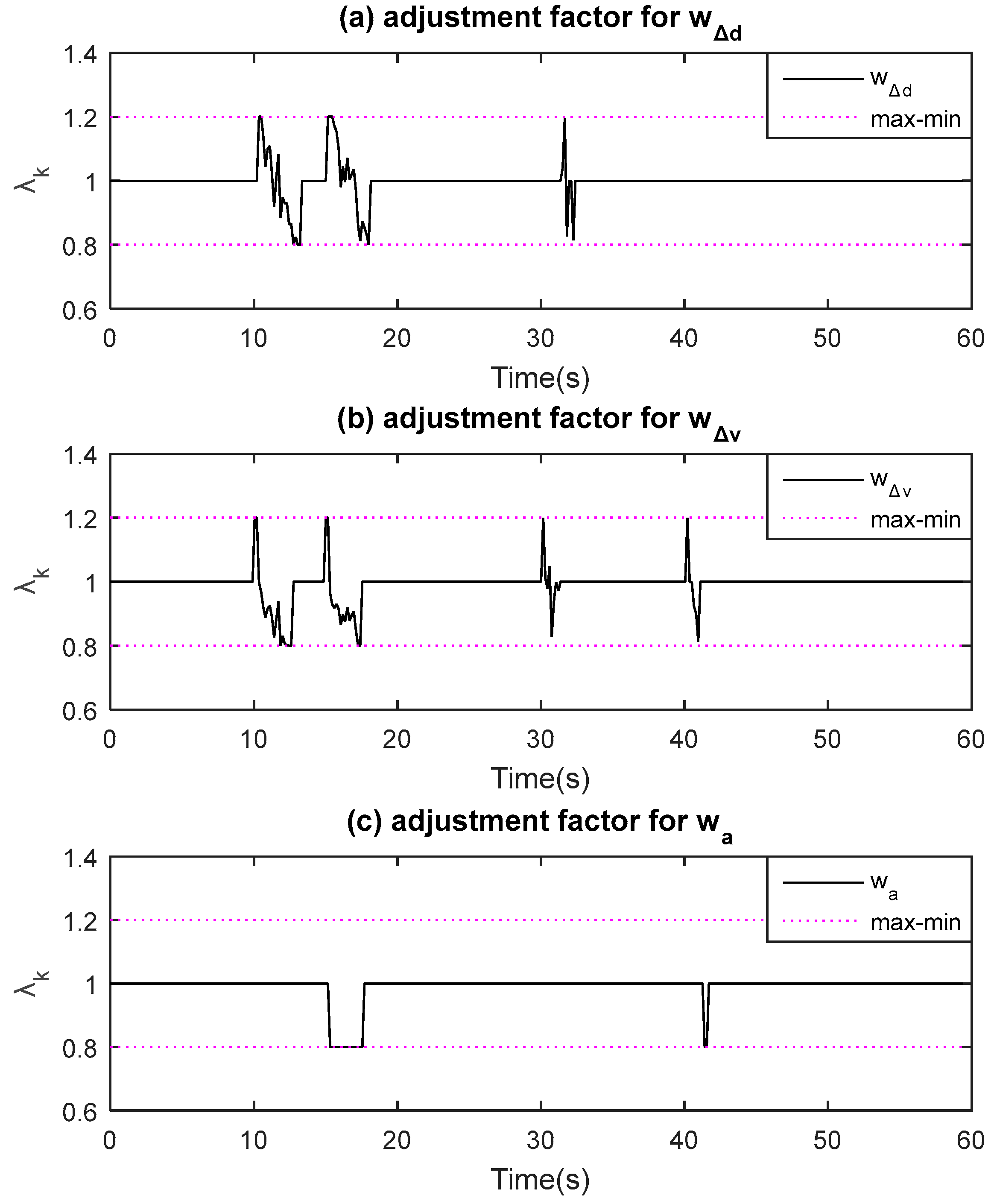
Figure 12.
Adhesion workload.


Table 1.
Parameters of the IACC Controller. IACC: integrated adaptive cruise control.
| Para. | Value | Para. | Value |
|---|---|---|---|
| 1.0 | 5 | ||
| 0.40 | −5 | ||
| 0.1 | 0.9 | ||
| −3 | −1.0 | ||
| 1.5 | 1.0 | ||
| 5 | −4.0 | ||
| 5 | 2 | ||
| p | 5 | −2 | |
| 1444 | 3 | ||
| 9.81 | −3 | ||
| 0.018 | 0.9 | ||
| 1.10 | −1.0 | ||
| 1.57 | 0.1 | ||
| 0.30 | −0.1 | ||
| 0 | 0.05 | ||
| 2.22 | −0.05 | ||
| 0.37 | diag(10,10,1,1,10,10) | ||
| 1750 | diag(1,1) | ||
| diag(3,3,3,3,3) |
© 2018 by the authors. Licensee MDPI, Basel, Switzerland. This article is an open access article distributed under the terms and conditions of the Creative Commons Attribution (CC BY) license (http://creativecommons.org/licenses/by/4.0/).
Share and Cite
MDPI and ACS Style
Zhang, J.; Li, Q.; Chen, D. Integrated Adaptive Cruise Control with Weight Coefficient Self-Tuning Strategy. Appl. Sci. 2018, 8, 978. https://doi.org/10.3390/app8060978
AMA Style
Zhang J, Li Q, Chen D. Integrated Adaptive Cruise Control with Weight Coefficient Self-Tuning Strategy. Applied Sciences. 2018; 8(6):978. https://doi.org/10.3390/app8060978
Chicago/Turabian StyleZhang, Junhui, Qing Li, and Dapeng Chen. 2018. "Integrated Adaptive Cruise Control with Weight Coefficient Self-Tuning Strategy" Applied Sciences 8, no. 6: 978. https://doi.org/10.3390/app8060978
Note that from the first issue of 2016, this journal uses article numbers instead of page numbers. See further details here.