Quantum Antenna as an Open System: Strong Antenna Coupling with Photonic Reservoir

School of Electrical Engineering, Tel Aviv University, Tel Aviv 39040, Israel
*
Author to whom correspondence should be addressed.
Appl. Sci. 2018, 8(6), 951; https://doi.org/10.3390/app8060951
Submission received: 25 April 2018
/
Revised: 29 May 2018
/
Accepted: 5 June 2018
/
Published: 8 June 2018
(This article belongs to the Special Issue Nano-Antennas)
Abstract
:We propose a general concept of quantum antenna in the strong coupling regime. It is based on the theory of open quantum systems. Antenna emission into space is considered an interaction with a thermal photonic reservoir. For antenna dynamics modeling, we formulate master equations with a corresponding Lindblad super-operators for the radiation terms. It is shown that strong coupling dramatically changes the radiation pattern of antenna. The total power pattern splits to three partial components, each of which corresponds to a spectral line in Mollow triplet. We analyzed the dependence of splitting on the length of antenna, shift of the phase, and Rabi-frequency. The predicted effect opens a way for implementation of multi-beam electrically tunable antennas, potentially useful in different nano-devices.
1. Introduction
Traditionally, the field of quantum optics deals with a control of quantum statistical correlations of light using elements such as interferometers, cavities, photonic crystals, beam splitters, etc. [1]. Purcell effect [2] and Dicke’s superradiance effect [3] are two of the most intriguing effects in quantum optics. Purcell predicted in 1946 the dependence of spontaneous emission rate on the environment of the light source. The effect is based on the ability of the specific environment to control the photonic density of states at the source position. In 1954, Dicke introduced the concept of enhanced spontaneous emission by an optically small ensemble of identical two-level atoms collectively interacting via a common electromagnetic field [3]. This effect involves the collective Dicke’s states which turn out to be highly entangled. The problem becomes even more fascinating if instead of a small atomic cloud, the size of the system becomes comparable to the wavelength. In 2006, Scully with co-workers focused on the problem of a single photon stored in a large cloud of atoms, which exists in a collective N-atom state [4,5,6,7,8,9]. The photon is shared among the atoms, thus one of them is excited, but we do not know which one. When the atoms in various positions are excited at different moments in time (Dicke’s states timing), the usual picture of collective emission, which treats each atom as a tiny antenna, is no longer valid. In this case, peculiar features of the directional and temporal characteristics of the cooperatively emitted radiation have been predicted. In particular, a single photon absorption by the cloud of N atoms is followed by the spontaneous emission in the same direction. These investigations gave birth to what is known today as “correlated spontaneous emission” and opened one of the possible ways for quantum antenna design.
Rapid progress in communication and radar technologies for the radio frequency ranges (from microwaves to terahertz) led to the development of various types of antennas that control electromagnetic fields on the wavelength scale [10,11,12,13]. The progress in modern nanotechnologies brings about the general trend of the transferring principles of radio-communication to the optical range. Thus, optical antennas became a promising tool for manipulating and controlling optical radiation [10,11,12,13].
In general, the classical antenna is defined as a device transforming the energy of coupled near field to the free far field (transmitting antennas) and vice versa (receiving antennas) [14]. Such a definition becomes unsuitable for nano-antennas of classical and quantum origin. The reason for this is that, in contrast to the classical case, the antenna emitters and detectors cannot be considered independently of the antenna’s elements. The radiation antenna properties are not separable from the source’s and detector’s origin. It becomes incorrect to speak about antennas as passive linear elements. Antennas become nonlinear and active (for recent reviews—see [15,16]). Antenna nonlinearities in their typical implementations are so strong that consideration of nonlinearity as a weak perturbation breaks down. Strong and even ultra-strong coupling of emitter and EM field became a reality [17]. As a result, such fundamental effects as spontaneous emission [18,19], Rabi-oscillations [20,21], and solitons [22,23] became the basis principles for quantum nano-antennas. The different types of nanostructures (plasmonic nanowires [24], quantum dots [25], carbon nanotubes [26,27,28], etc.) have been considered as promising models for their implementation. As a result, a new way is opened for antenna’s design control by directed quantum emission and correlation of light properties [29]. In many cases the effect of non-reciprocity manifests itself in quantum antennas [30,31], which leads to the difference of the same antenna’s properties in transmitting and receiving regimes without using the ordinary types of non-reciprocal materials. On the other hand, the quantum origin leads to some fundamental limitations, which are not installation-specific classical antennas (for example, Heisenberg uncertainty principle [32]).
The classical antenna concept is based on such conventional parameters as a field radiation pattern, power pattern, radiation resistance, directivity, gain, etc. [14]. All these values are completely defined by the current distribution of the antenna. The field and power patterns are exactly square-law coupled. In the quantum case, the field and power are defined as expectation values of the corresponding photonic operators [1] with respect to the quantum states of antenna emitter. As a result, the coupling between observable fields and powers becomes unobvious and strongly dependent on the initial state of emitter. It should be taken into account when introducing the conventional antenna parameters mentioned above. On the other hand, the quantum antennas pen the way for producing the quantum light with special coherent properties. For example, for the two particle entangled states of antenna, the directional photon pairs emission that are strongly correlated in momentum were predicted [29]. It requires an introduction of some other antenna’s characteristics, which do not have classical analogs, such as the second-order correlation photonic functions [29]. Still incomplete, this list shows that conventional antenna concepts [14] need a fundamental reconsideration when dealing with quantum antenna design.
In this paper, we focus on the theory of quantum-optical antenna with fermionic type of excitation. Our description is based on such general principles of quantum physics as theory of open systems [1,33] with their bridging to the classical antenna theory [14]. The general principle of open system theory is based on the separation of the actual system and evanescent space (reservoir). The last one assumed to be so large that its interaction with the actual system does not change its quantum state. We consider the quantum antenna as a radiating actual system and a surrounding space in which radiation takes place—as a reservoir. The interaction between the actual system and reservoir leads to losses in the former. Therefore, the theory of open systems is an effective general technique for description of losses of different physical origin and may be applied to the problem of antenna emission. The antenna’s emission has been considered as a loss of energy of a source placed in space (this is the place to speak about radiative losses). The influence of antenna on the state of surrounding area is negligibly small. Therefore, the later may be considered as photonic reservoir. The model of photonic reservoir in the thermal state corresponds to the transmitting antenna (the antenna’s evanescent field appears in a thermal equilibrium state and produces the thermal noise). Our considerations have yielded the fundamental properties of quantum antennas, which have no analogs in the classical ones and provide applications in the future.
The paper is organized as follows: in Section 2 we formulate the model of quantum antenna as a quantum system, and formulate the basis Hamiltonian and corresponding master equation. In Section 3, we study the dynamics of quantum antenna basing on the approximate analytical solutions in the regimes of weak and strong coupling. The power radiative patterns of quantum antenna are studied in Section 4. The conclusions, main results, and their promising applications are formulated in Section 5.
2. Model of Quantum Antenna as an Open System
The general model of the antenna is shown in Figure 1. We consider the antenna as a quantum dot placed inside a quantum wire which behaves as a waveguide (Figure 1a). Such structures were implemented experimentally in the form of tapered InP nanowire waveguide containing a single InAsP quantum dot [34,35,36]. The quantum dot is perfectly positioned on the axis of InP nanowire waveguides, where the emission is efficiently coupled to the fundamental waveguide mode.
From a theoretical point of view, this system may be considered as a defect of a crystal lattice. Therefore, the general model of the bulk crystal defects, which is based on Wannier functions [37], may be used for the antenna analysis. Similarly to [37], we define Wannier functions mutually coupled to Bloch functions via relations
where is a number of zone and is a quasi-momentum of the charge. The Wannier function is strongly localized in the vicinity of the atom at the point . An arbitrary wave-function is given by , where the envelope in the continuous limit satisfies the Schrodinger equation
where is the potential, averaged with respect to the crystal lattice, and and are the effective mass and energy of charge carrier, respectively.
The Bloch function may be presented as , where is a periodic function such that . The Wannier and Bloch states satisfy the uncertainty principle [37] in the form . This means that, for rather long antenna (large ), the main support to the wave-function is defined by a small region near the band minimum at the zone center. As a result, we obtain the approximate presentation for the wave function at the given zone
Equation (4) shows that the quantum properties of antenna may be modeled by a two-level artificial atom with Fermionic quantum states , separated by the energy with the same spatial envelope (Figure 1b).
We assume the length of antenna to be comparable to the wavelength. The area of quantum confinement is also comparable to a wavelength. It makes the retardation of EM field in its interaction with quantum emitter to be essential. The antenna is driven by the classical external field in the regime of arbitrary coupling. Particularly, an essential role in the formation of radiation is played by the Rabi-oscillations produced by the antenna feeding. Therefore, its interaction with the EM field cannot be considered by different types of perturbation theories.
The total Hamiltonian of antenna in the EM-field within the bounds of given model is , where
is Hamiltonian of free antenna and
is the interaction Hamiltonian with the external field. We will limit our consideration to the strong coupling regime and not consider the ultra-strong one [17], thus Hamiltonian (6) is written in rotating-wave approximation [1]. The states are the excited and ground states of antenna without field, are the frequencies of optical transition and driven field, respectively and is the Rabi-frequency.
The radiation of quantum antenna coupled to photonic reservoir is described in rotating-wave approximation [1] by Hamiltonian
where is a coupling factor of k-th EM-field mode of reservoir with antenna, is the dipole moment, is a Fermionic-type lowering operator of antenna excitation, is a creation operator of photon in the k-th mode, is the unit vector along the antenna axis, are the frequency and wave-vector of k-th mode, respectively and is the normalization volume.
We will use the Eigenfunctions of Hamiltonian as a basis functions. For this, we transform all operators according to , where is the transformation operator. The transformed Hamiltonian components are and , where is the frequency detuning. The Eigenmodes are defined by relation where The eigenvalues are given by , with corresponding Eigenmodes
where is a normalization factor and . The Eigenmodes (8) and (9) are orthonormal: . These states describe the interaction of excited and ground states via Rabi-oscillations with frequency .
The state of emitting antenna is characterized by a density matrix, , which satisfies the master equation
The last term is the Lindblad super-operator which models antenna emission as its coupling to a photonic thermal reservoir. It reads in its conventional form
The next step of simplification consists in the standard transition from summation over to the frequency integration [1] using the replacement
where azimuthal integration have been carried out and the new variable of integration have been used. As a result, we obtain
where
The main support to the time integral is given by the narrow vicinity of frequencies . It allows us to use the approximation and integrate using . Thus, we have
The relaxation parameter is a spontaneous emission frequency. Its difference from Weisskopf–Wigner result for individual atoms [1] consists in the special interference dictated by the relative phase shift of different EM-modes over antenna axis. As a result, its frequency dependence does not add up to as for the case of individual atom.
The presentation of operator at the basis (8) and (9) reads
where coefficients are elements of matrix . The equations of density matrix elements in the basis (8) and (9) are
The relaxation parameters are obtained from rather long, but trivial calculations. They are given by
The element may be found from the probability conservation law [1].
3. Dynamics of Quantum Antenna: Qualitative Analysis
The strong coupling regime corresponds to the condition , which gives . For simplicity, we will analyze the antenna dynamics in the regime of exact resonance (zero detuning). In this case the approximations , , become appropriate. Therefore, the system (9)–(11) simplifies to
The system (25)–(27) is equal to the equations of resonant fluorescence [1]. The temporal evolution described by this system goes to the steady state defined by the condition . For the strong fields such that the last two terms in [1] have been neglected. As a result, the steady state values and . We are keeping these terms and obtain the steady state as
where
As it follows from (20), the antenna emission has not vanished, while the emission properties are independent on its initial state.
4. Radiation Properties of Quantum Antenna
In this section, we will consider the power radiation pattern of quantum antenna in the strong coupling regime. The far field emitted by antenna [1] presented as a superposition of the partial supports produced by elementary dipoles induced at the antenna surface. The positive-frequency part of field operator produced by the single dipole quantum emitter [1] in spherical system is given by , where is the spherical radial coordinate (dipole assumed to be placed at the origin). The corresponding operator of the antenna field is given by
The normally ordered operator of intensity in the far field zone is given by
The observable value of intensity is expressed through the two-time correlation function of polarization [1]. It reads
where
We will consider the steady state of antenna given by Equations (23) and (24). It is a stationary process for which the correlation function is time-independent. Thus, Equation (28) may be rewritten as
The correlation function (29) is equal to the correlation function of resonance fluorescence considered in detail in [1]. An approximate relation for steady state is given by
where . The time shift in antenna is stipulated by the phase shift of radiation from different points and is given by . For simplifying the integration in (27), we will use the conventional assumptions from macroscopic antenna theory [14]
for amplitude and phase factors, respectively, where are coordinates for the spherical system with origin at the antenna center (exponentially attenuated factors in (30) are related to the amplitude and thus approximated according to (36). As a result, the intensity of radiation may be presented in terms of radiation pattern from conventional antenna theory [14]. It reads
where
().
For illustrating the qualitative properties of radiation pattern we consider the simplest model of perfect linear antenna [14], quantum envelope of which has the constant spatial amplitude and the linear phase distribution , where is a normalized phase shift per unit length. The integration in (33) gives
with , .
Let us consider now the angular pattern of power spectrum of quantum antenna for the strong-field limit (). Following Wiener–Khintchine theorem, it is given in terms of the two-time correlation function by the field in the far zone by
where
Making the integrations in (35) and (36), we obtain the final result in the form
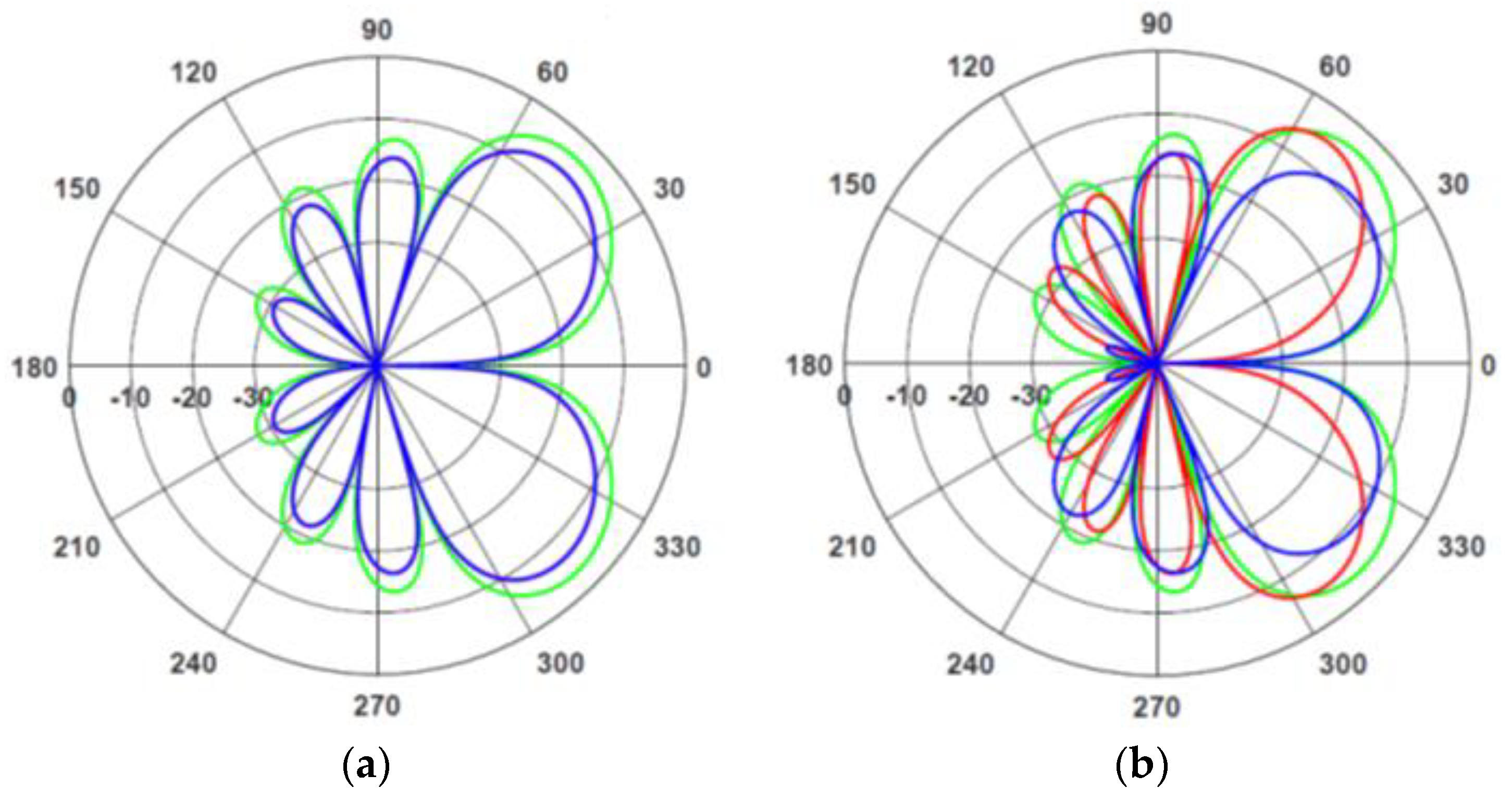
Equation (37) allows us to analyze the qualitative behavior of radiation pattern, some aspects of which are seen to be in agreement with theory of resonance fluorescence [1]. The total radiation pattern represents the sum of three elementary patterns having the form of perfect wire antenna [14], centered at the three different angles , . The weight of the elementary pattern is defined by the corresponding resonant line centered at one of the frequencies , , . Such a form of frequency spectrum corresponds to a Mollow triplet in resonance fluorescence for the case of strong driving field [1]. The element of novelty in the antenna is that the radiation of each triplet-line occurs in its own direction. The value of angle splitting depends on the driving field, phase shift of the quantum envelope along antenna, and its length compared to the wavelength.
The trends of mentioned behavior are illustrated in Figure 2, Figure 3 and Figure 4. The elementary radiation patterns of the lines (colored green), (colored red), and (colored blue) in logarithmic scale for different values of various parameters have been shown in these Figures. The patterns are in the ratio 2:1:1 according to the ratio of integrated intensities in the peaks. It means that every elementary pattern corresponds to the signal formed by the broadened spectral line with the width , respectively. Figure 2a corresponds approximately to the typical pattern of a wire antenna. The lines that correspond to and not seen separately since are merged for such a small value of driving field. A rather small difference between the powers of central line and side ones is observed, but not such a case for angle splitting. Increasing of Rabi-frequency (Figure 2b) does not change the number of lobes but leads to an angle splitting of rather small value for the side lobes.
The patterns become more and more jagged with the increase of length (Figure 3 and Figure 4). Simultaneously, the effect of pattern separation increases and even the absolute separation becomes reachable (the angle of maximum for the main lobe of one pattern coincides with the minimum for another one). The typical radiation patterns of wire antennas are highly dependent on the value of phase shift. The value defines the regime of axial radiation. For the phase shift exceeding the critical value , the main lobe moves to the invisible region [14] and disappears from the observable range of angles . Therefore, the antenna emission is completely formed out of a superposition of side lobes, which are not coherent. As a result, the emitted power decreases, making this regime unsuitable for a lot of applications. For classical wire antennas [14]. In our case we have own critical shift for each partial diagram: for central line and for two side lines. The last two critical values depend on Rabi-frequency and become controllable via the adiabatic field variation. For example, the right-hand line may be removed to the invisible region while the two others are left in the visible one. This mechanism manifests itself in the strong decrease of the emitted power at the line compared to two others for rather large Rabi-frequency (Figure 3a and Figure 4a).
The conventional antenna parameters—such as directivity, gain, etc. [14]—may be defined by the ordinary way for the quantum antenna considered in this paper. However, it is more natural to consider separately each component of Mollow triplet. For the side lobes (the two last terms in Equation (37)) these values will depend on the driving electromagnetic field.
5. Conclusions
In summary, we developed a model of quantum antenna in the strong coupling regime basing on the general theory of open quantum systems [1,33]. The far-field zone of antenna radiation is considered as the thermal photonic reservoir. We formulated and solved the master equation with Lindblad-terms related to the energy losses via antenna emission. The general concept was applied to the wire antenna with Fermionic type of excitation. Spectral density of power in the far-field zone was calculated. It is shown that the strong coupling regime dramatically changes the radiation pattern compared to the macroscopic antennas and optical nano-antennas of different well-known types. The calculated radiation pattern consists out of three components, each of which corresponds to the resonance line in the Mollow triplet and turned one with respect to another at some angle. The value of this angle strongly depends on the geometric parameters of antenna, energy spectra of used materials, and the value of coupling (Rabi-frequency). It opens new ways for highly effective electric control of antenna’s characteristics for using in different nano-photonic applications. On the other hand, the influence of EM field on the pattern should be accounted from the point of view of electromagnetic compatibility in nanoscale [38,39].
Author Contributions
Developments of the physical models, derivation of the basis equations, interpretation of the physical results, and paper writing have been done by A.K. and G.S. jointly.
Conflicts of Interest
The authors declare no conflict of interest.
References
- Scully, M.O.; Zubairy, M.S. Quantum Optics; Cambridge University Press: Cambridge, UK, 2001. [Google Scholar]
- Purcell, E.M.; Torrey, H.C.; Pound, R.V. Resonance Absorption by Nuclear Magnetic Moments in a Solid. Phys. Rev. 1946, 69, 37. [Google Scholar] [CrossRef]
- Dicke, R.H. Coherence in Spontaneous Radiation Processes. Phys. Rev. 1954, 93, 99. [Google Scholar] [CrossRef]
- Scully, M.O. Collective Lamb Shift in Single Photon Dicke Superradiance. Phys. Rev. Lett. 2009, 102, 143601. [Google Scholar] [CrossRef] [PubMed]
- Scully, M.O. Single Photon Subradiance: Quantum Control of Spontaneous Emission and Ultrafast Readout. Phys. Rev. Lett. 2015, 115, 243602. [Google Scholar] [CrossRef] [PubMed]
- Scully, M.O.; Fry, E.S.; Ooi, C.R.; Wódkiewicz, K. Directed Spontaneous Emission from an Extended Ensemble of N Atoms: Timing Is Everything. Phys. Rev. Lett. 2006, 96, 010501. [Google Scholar] [CrossRef] [PubMed]
- Svidzinsky, A.A.; Chang, J.-T.; Scully, M.O. Cooperative spontaneous emission of N atoms: Many-body eigenstates, the effect of virtual Lamb shift processes, and analogy with radiation of N classical oscillators. Phys. Rev. A 2010, 81, 053821. [Google Scholar] [CrossRef]
- Svidzinsky, A.A.; Chang, J.-T.; Scully, M.O. Dynamical Evolution of Correlated Spontaneous Emission of a Single Photon from a Uniformly Excited Cloud of N Atoms. Phys. Rev. Lett. 2008, 100, 160504. [Google Scholar] [CrossRef] [PubMed]
- Das, S.; Agarwal, G.S.; Scully, M.O. Quantum Interferences in Cooperative Dicke Emission from Spatial Variation of the Laser Phase. Phys. Rev. Lett. 2008, 101, 153601. [Google Scholar] [CrossRef] [PubMed]
- Biagioni, P.; Huang, J.-S.; Hecht, B. Nanoantennas for visible and infrared radiation. Rep. Prog. Phys. 2012, 75, 024402. [Google Scholar] [CrossRef] [PubMed] [Green Version]
- Novotny, L.; van Hulst, N. Antennas for light. Nat. Photonics 2011, 5, 83. [Google Scholar] [CrossRef]
- Alu, A.; Engheta, N. Input Impedance, Nanocircuit Loading, and Radiation Tuning of Optical Nanoantennas. Phys. Rev. Lett. 2008, 101, 043901. [Google Scholar] [CrossRef] [PubMed]
- Greffet, J.-J.; Laroche, M.; Marquier, F. Impedance of a Nanoantenna and a Single Quantum Emitter. Phys. Rev. Lett. 2010, 105, 117701. [Google Scholar] [CrossRef] [PubMed]
- Balanis, K. Antenna Theory; John Wiley and Sons, Inc.: New York, NY, USA, 1997. [Google Scholar]
- Chen, P.-Y.; Argyropoulos, C.; Alù, A. Enhanced nonlinearities using plasmonic nanoantennas. Nanophotonics 2012, 1, 221–233. [Google Scholar] [CrossRef]
- Monticone, F.; Argyropoulos, C.; Alù, A. Optical antennas, Controlling electromagnetic scattering, radiation, and emission at the nanoscale. IEEE Antennas Propag. Mag. 2017, 59, 43–61. [Google Scholar] [CrossRef]
- Todorov, Y.; Sirtori, C. Few-electron ultrastrong light-matter coupling in a quantum LC Circuit. Phys. Rev. X 2014, 4, 041031. [Google Scholar]
- Mokhlespour, S.; Haverkort, J.E.M.; Slepyan, G.; Maksimenko, S.; Hoffmann, A. Collective spontaneous emission in coupled quantum dots: Physical mechanism of quantum nanoantenna. Phys. Rev. B 2012, 86, 245322. [Google Scholar] [CrossRef]
- Egglestona, M.S.; Messera, K.; Zhangb, L.; Yablonovitch, E.; Wu, M.C. Optical antenna enhanced spontaneous emission. Proc. Natl. Acad. Sci. USA 2015, 112, 1704–1709. [Google Scholar] [CrossRef] [PubMed] [Green Version]
- Slepyan, G.Y.; Yerchak, Y.D.; Hoffmann, A.; Bass, F.G. Strong electron-photon coupling in a one-dimensional quantum dot chain: Rabi waves and Rabi wave packets. Phys. Rev. B 2010, 81, 085115. [Google Scholar] [CrossRef]
- Slepyan, G.Y.; Yerchak, Y.D.; Maksimenko, S.A.; Hoffmann, A.; Bass, F.G. Mixed states in Rabi waves and quantum nanoantennas. Phys. Rev. B 2012, 85, 245134. [Google Scholar] [CrossRef]
- Gligorić, G.; Maluckov, A.; Hadžievski, L.; Slepyan, G.Y.; Malomed, B.A. Discrete solitons in an array of quantum dots. Phys. Rev. B 2013, 88, 155329. [Google Scholar] [CrossRef] [Green Version]
- Gligorić, G.; Maluckov, A.; Hadžievski, L.; Slepyan, G.Y.; Malomed, B.A. Soliton nanoantennas in two-dimensional arrays of quantum dots. J. Phys. Condens. Matter 2015, 27, 225301. [Google Scholar] [CrossRef] [PubMed] [Green Version]
- Agio, M.; Alu, A. Optical Antennas; Cambridge University Press: Cambridge, UK, 2013. [Google Scholar]
- Gaponenko, S.V. Introduction to Nanophotonics; Cambridge University Press: Cambridge, UK, 2010. [Google Scholar]
- Hanson, G. Fundamental transmitting properties of carbon nanotube antennas. IEEE Trans. Antennas Propag. 2005, 53, 3426–3435. [Google Scholar] [CrossRef] [Green Version]
- Slepyan, G.Y.; Shuba, M.V.; Maksimenko, S.A.; Lakhtakia, A. Theory of optical scattering by achiral carbon nanotubes and their potential as optical nanoantennas. Phys. Rev. B 2006, 73, 195416. [Google Scholar] [CrossRef]
- Ren, L.; Zhang, Q.; Pint, C.L.; Wójcik, A.K.; Bunney, M., Jr.; Arikawa, T.; Kawayama, I.; Tonouchi, M.; Hauge, R.H.; Belyanin, A.A.; et al. Collective antenna effects in the terahertz and infrared response of highly aligned carbon nanotube arrays. Phys. Rev. B 2013, 87, 161401. [Google Scholar] [CrossRef] [Green Version]
- Mikhalychev, A.; Mogilevtsev, D.; Slepyan, G.Y.; Karuseichyk, I.; Buchs, G.; Boiko, D.L.; Boag, A. Synthesis of Quantum Antennas for Shaping Field Correlations. Phys. Rev. Appl. 2018, 9, 024021. [Google Scholar] [CrossRef] [Green Version]
- Slepyan, G.Y.; Boag, A. Quantum Nonreciprocity of Nanoscale Antenna Arrays in Timed Dicke States. Phys. Rev. Lett. 2013, 111, 023602. [Google Scholar] [CrossRef] [PubMed]
- Caloz, C.; Alu, A.; Tretyakov, S.; Sounas, D.; Achouri, K.; Leger, Z.-L.D. What is Nonreciprocity? Part II. arXiv 2018, arXiv:1804.00238. [Google Scholar]
- Slepyan, G.Y. Heisenberg uncertainty principle and light squeezing in quantum nanoantennas and electric circuits. J. Nanophoton. 2016, 10, 046005. [Google Scholar] [CrossRef]
- Breuer, H.-P.; Petruccione, F. The Theory of Open Quantum Systems; Oxford University Press: Oxford, UK, 2007. [Google Scholar]
- Reimer, M.E.; Bulgarini, G.; Akopian, N.; Hocevar, M.; Bavinck, M.B.; Verheijen, M.A.; Bakkers, E.P.A.M.; Kouwenhoven, L.P.; Zwiller, V. Bright single-photon sources in bottom-up tailored nanowires. Nat. Commun. 2012, 3, 737. [Google Scholar] [CrossRef] [PubMed] [Green Version]
- Bulgarini, G.; Reimer, M.E.; Zehender, T.; Hocevar, M.; Bakkers, E.P.; Kouwenhoven, L.P.; Zwiller, V. Spontaneous emission control of single quantum dots in bottom-up nanowire waveguides. Appl. Phys. Lett. 2012, 100, 121106. [Google Scholar] [CrossRef] [Green Version]
- Van Weert, M.H.; Akopian, N.; Perinetti, U.; van Kouwen, M.P.; Algra, R.E.; Verheijen, M.A.; Bakkers, E.P.A.M.; Kouwenhoven, L.P.; Zwiller, V. Selective Excitation and Detection of Spin States in a Single Nanowire Quantum Dot. Nano Lett. 2009, 9, 5. [Google Scholar] [CrossRef] [PubMed]
- Yu, P.; Cardona, M. Fundamentals of Semiconductors: Physics and Material Properties; Springer: Berlin/Heidelberg, Germany, 2001. [Google Scholar]
- Slepyan, G.; Boag, A.; Mordachev, V.; Sinkevich, E.; Maksimenko, S.; Kuzhir, P.; Miano, G.; Portnoi, M.E.; Maffucci, A. Anomalous electromagnetic coupling via entanglement at the nanoscale. New J. Phys. 2017, 19, 023014. [Google Scholar] [CrossRef] [Green Version]
- Slepyan, G.Y.; Boag, A.; Mordachev, V.; Sinkevich, E.; Maksimenko, S.; Kuzhir, P.; Maffucci, A. Nanoscale electromagnetic compatibility: quantum coupling and matching in nanocircuits. IEEE Trans. Electromagn. Compat. 2015, 57, 1645–1654. [Google Scholar] [CrossRef]
Figure 1.
General illustration of the system used as a model of quantum antenna in the strong coupling regime. (a) The antenna configuration. The semiconductor InAsP quantum dot (red colored) positioned inside the semiconductor InP quantum wire (green colored). The quantum dot is coupled with quantum wire via quantum tunneling through the potential barriers. (b) The energy spectrum of the shown system in the case of EM field absence. It consists of two zones, valence and conduction, which are separated by the energy gap. The dominant support to the energy of quantum transitions is given by the small region near the band minimum at the zone center and is approximately equal to .
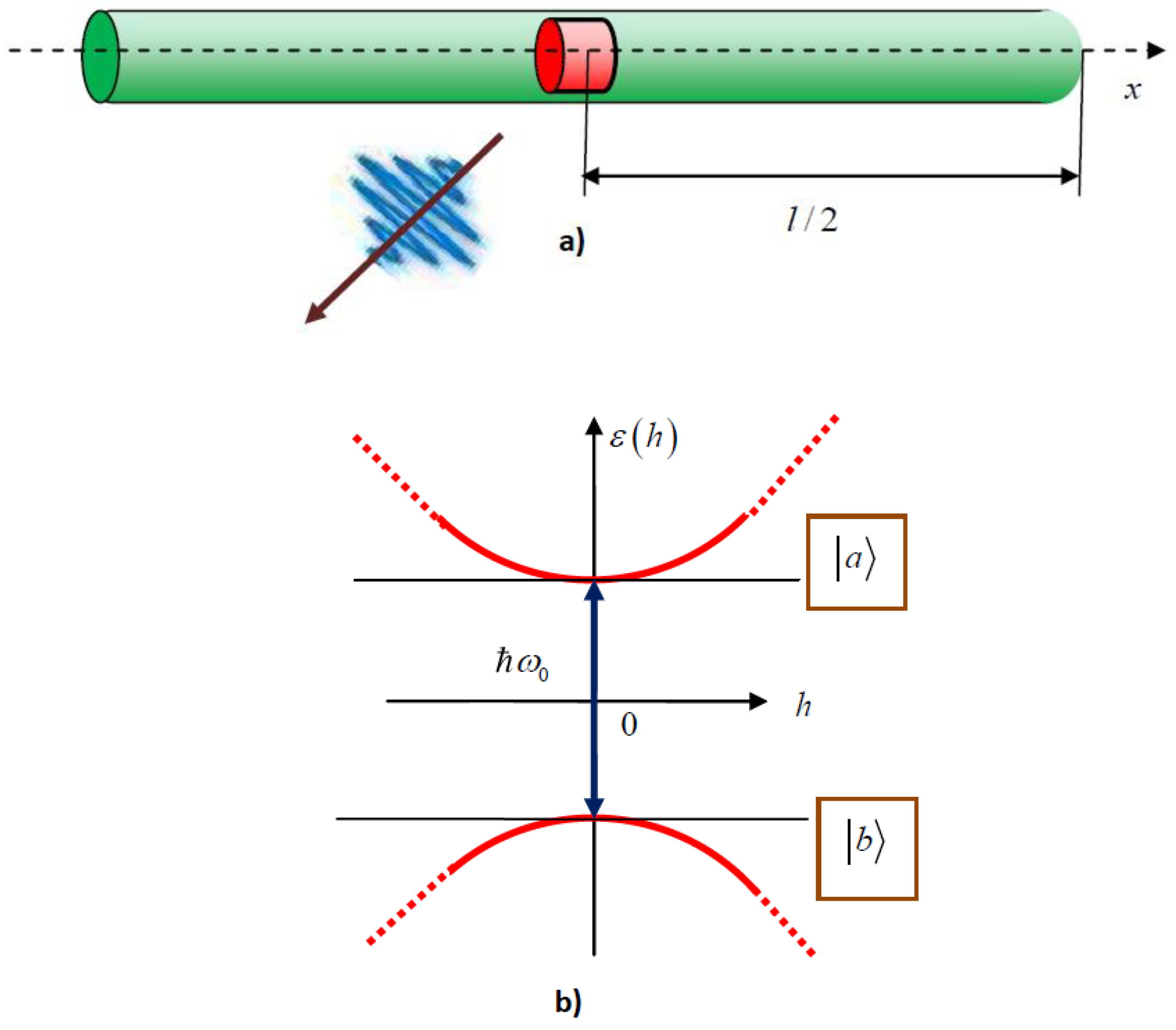
Figure 2.
The elementary radiation patterns of the lines (green), (red), and (blue) for different values of Rabi-frequency. The patterns are in the ratio 2:1:1 according to the ratio of integrated intensities in the peaks. The patterns are presented in logarithmic scale. . (a) ; (b) .
Figure 2.
The elementary radiation patterns of the lines (green), (red), and (blue) for different values of Rabi-frequency. The patterns are in the ratio 2:1:1 according to the ratio of integrated intensities in the peaks. The patterns are presented in logarithmic scale. . (a) ; (b) .

Figure 3.
The elementary radiation patterns of the lines (green), (red) and (blue) in logarithmic scale for different values of phase shift. . (a) ; (b) .
Figure 3.
The elementary radiation patterns of the lines (green), (red) and (blue) in logarithmic scale for different values of phase shift. . (a) ; (b) .
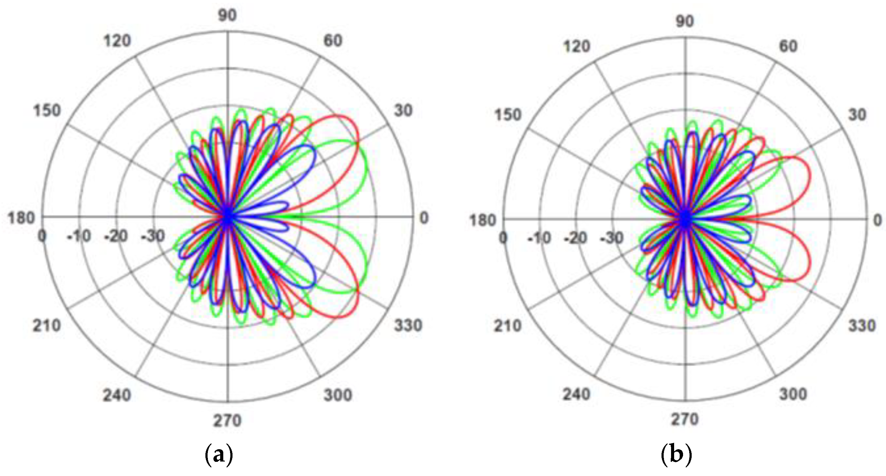
Figure 4.
The elementary radiation patterns of the lines (green), (red), and (blue) in logarithmic scale for different values of phase shift. . (a) ; (b) .
Figure 4.
The elementary radiation patterns of the lines (green), (red), and (blue) in logarithmic scale for different values of phase shift. . (a) ; (b) .

© 2018 by the authors. Licensee MDPI, Basel, Switzerland. This article is an open access article distributed under the terms and conditions of the Creative Commons Attribution (CC BY) license (http://creativecommons.org/licenses/by/4.0/).
Share and Cite
MDPI and ACS Style
Komarov, A.; Slepyan, G. Quantum Antenna as an Open System: Strong Antenna Coupling with Photonic Reservoir. Appl. Sci. 2018, 8, 951. https://doi.org/10.3390/app8060951
AMA Style
Komarov A, Slepyan G. Quantum Antenna as an Open System: Strong Antenna Coupling with Photonic Reservoir. Applied Sciences. 2018; 8(6):951. https://doi.org/10.3390/app8060951
Chicago/Turabian StyleKomarov, Alexei, and Gregory Slepyan. 2018. "Quantum Antenna as an Open System: Strong Antenna Coupling with Photonic Reservoir" Applied Sciences 8, no. 6: 951. https://doi.org/10.3390/app8060951
Note that from the first issue of 2016, this journal uses article numbers instead of page numbers. See further details here.