Analytical Modeling for Underground Risk Assessment in Smart Cities


Computer Engineering Department, Jeju National University, Jeju-si 63243, Korea
*
Author to whom correspondence should be addressed.
Appl. Sci. 2018, 8(6), 921; https://doi.org/10.3390/app8060921
Submission received: 16 April 2018
/
Revised: 18 May 2018
/
Accepted: 24 May 2018
/
Published: 4 June 2018
Abstract
:In the developed world, underground facilities are increasing day-by-day, as it is considered as an improved utilization of available space in smart cities. Typical facilities include underground railway lines, electricity lines, parking lots, water supply systems, sewerage network, etc. Besides its utility, these facilities also pose serious threats to citizens and property. To preempt accidental loss of precious human lives and properties, a real time monitoring system is highly desirable for conducting risk assessment on continuous basis and timely report any abnormality before its too late. In this paper, we present an analytical formulation to model system behavior for risk analysis and assessment based on various risk contributing factors. Based on proposed analytical model, we have evaluated three approximation techniques for computing final risk index: (a) simple linear approximation based on multiple linear regression analysis; (b) hierarchical fuzzy logic based technique in which related risk factors are combined in a tree like structure; and (c) hybrid approximation approach which is a combination of (a) and (b). Experimental results shows that simple linear approximation fails to accurately estimate final risk index as compared to hierarchical fuzzy logic based system which shows that the latter provides an efficient method for monitoring and forecasting critical issues in the underground facilities and may assist in maintenance efficiency as well. Estimation results based on hybrid approach fails to accurately estimate final risk index. However, hybrid scheme reveals some interesting and detailed information by performing automatic clustering based on location risk index.
1. Introduction
Globally, urbanization is taking place in many countries. More job opportunities, better healthcare, education and entertainment facilities along with other privileges, attracts people living in rural areas for permanent migration. Rapid population growth in urban areas puts more pressure on available resources in city areas which results in pollution, traffic congestion and environmental degradation. In every big city, land is one of most precious resource and, to overcome this challenge, underground facilities are increasing day-by-day, as it is considered an improved utilization of available space in smart cities. Typical facilities include underground railway lines, parking lots, electric and water supply, sewerage lines, etc. Besides its utility, these facilities also pose serious threats to citizens and property. Despite care and precautions, many severe and unfortunate incidents have happened in underground facilities around the globe. Besides natural disasters, technical faults and human mistakes, there are other silent factors which pose constant and serious threats, e.g., continuous leakage of water and sewerage supply lines, structure fault and underground soil deformation. In most cases, the damage does not happen at once, rather the hazard builds up slowly and gradually behind the scene as many underground facilities are invisible and inaccessible. This is mainly attributed to poor construction and the slow degradation process in underground facility structures and materials due to continuous deterioration effects of weathering, aging, chemicals processes, corrosion, etc. [1,2]. To avoid any accidental loss, a sensor based real time monitoring system is highly desirable to conduct automated and continuous risk assessment to report any abnormality before it happens.
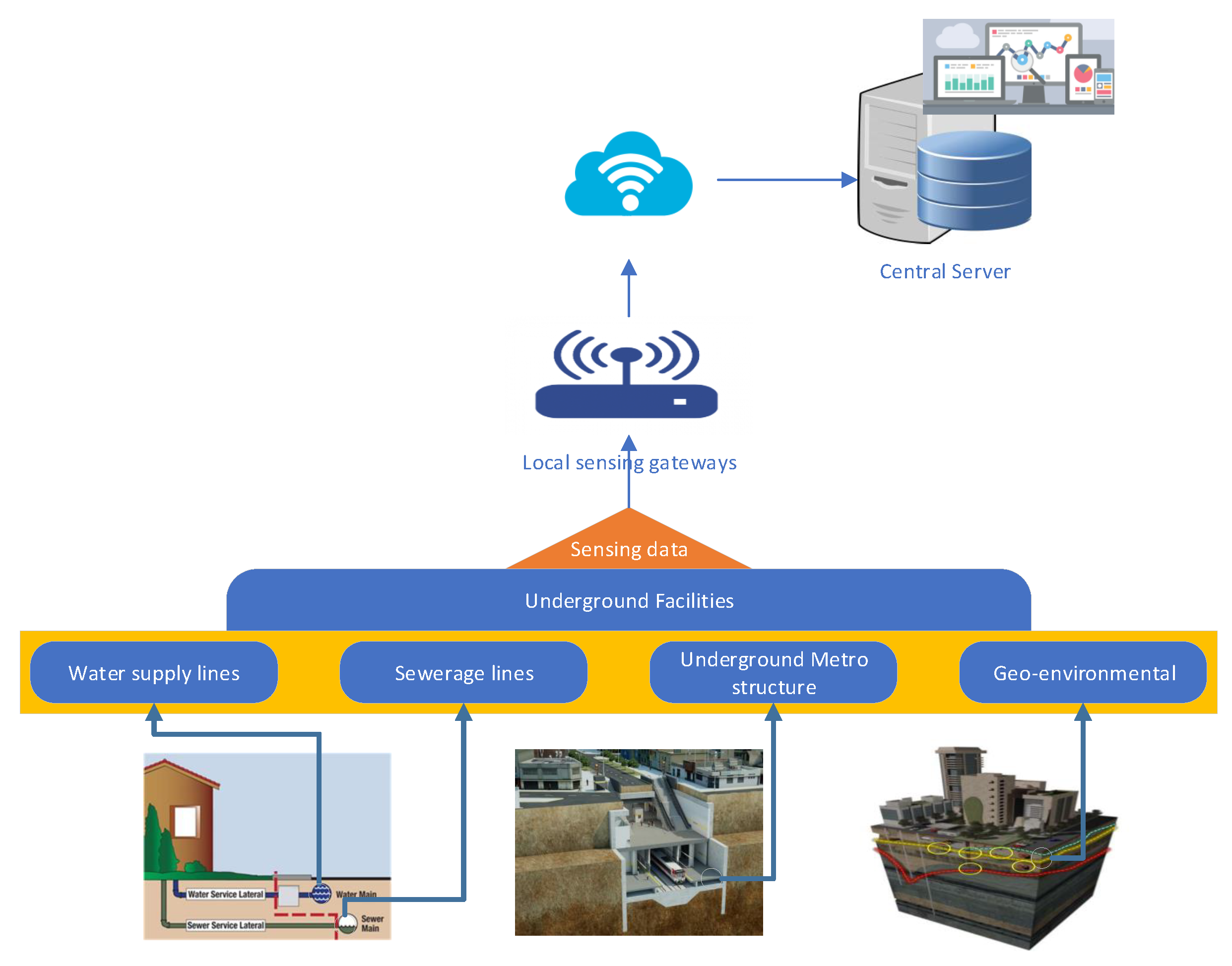
Risk at any location, at any point in time, depends on various associated factors, e.g., ground status, pipeline leakage, structure health, etc. These individual risk factors are referred to here as risk contributing factors (RCFs). Each RCF contributes towards final risk index (FRI) at that particular location. For underground risk analysis and assessment, the first step is to collect data about parameters of interest (i.e., RCF) via sensors deployed at selected locations. Risk index value of each individual factor is calculated by fusion and aggregation of relevant sensors data after necessary processing. Figure 1 shows the conceptual design for risk assessment of underground facilities. In a given geographical area, sensors are installed at selected locations for monitoring and risk assessment. Every RCF demands its own set of sensors. For example, water supply pipeline leakage is a risk contributing factor and its risk index is estimated by pressure sensors, flow sensors, and leakage sensors, as shown in Figure 1.
Several risk contributing factors are involved in underground risk assessment, each having its own risk index values. We need a single risk index value for a given location that is somehow representative of risk index values of all risk contributing factors. There is no known formulation to get final risk index from associated risk contributing factors and the actual relationship can be very complex in reality. Several approaches are adopted in the literature to address this problem. A brief summary of some related techniques is presented in next section. Normally, subjective risk assessment can be done by experts by visiting the site and observing the risk point. Besides subjectivity, manual risk assessment is very time consuming and costly.
Nonlinear and complex nature of relationship between risk score and risk rating contributing factors and corresponding final risk index demands an analytical modeling of the system. In this paper, we present analytical modeling for three different approximation schemes for estimation of final risk index from associated risk contributing factors: (a) simple linear approximation based on weights assignment to each factor; (b) hierarchical fuzzy logic based technique in which related risk factors are combined through fuzzy sub-systems in a tree like structure; and (c) hybrid approximation approach which is a combination of (a) and (b). Comprehensive evaluation of the proposed approximation is done using data for 100 underground facilities. Integrated hierarchical fuzzy inference system with maximum based rule definition scheme provides the best results, which gives us confidence to further explore this approach in the future. Hybrid scheme proves to be an effective approach for performing automatic clustering based on location risk index.
The rest of this paper is organized as follows: Brief description of related work is covered in Section 2. Problem formulation for underground risk assessment is done in Section 3. Afterwards, we present our approximation schemes in Section 4. Section 5 is about experimental design for evaluation of approximation schemes. A brief description about the implementation of proposed approximation schemes is given in Section 6. Section 7 is dedicated to performance analysis and discussion on results. Finally, we conclude this paper with an outlook to our future work in Section 8.
2. Related Work
Despite care and precautions, many severe and unfortunate incidents have happened in underground facilities around the globe. Investigation reveals that the major causes of incidents include natural disasters, technical faults, human mistakes and underground leakage and soil deformation. Improved structural design and strict adherence to standard operational procedures can help in building safer and disaster resilient communities. Designing for disaster is a platform for engineers, designers, planners, environmentalists and others to share their experiences by showcasing their innovative research findings [3]. Here, we try to address and design solutions for silent risk factors that pose constant and serious threats, e.g., continuous leakage of water and sewerage supply lines, structure fault and underground soil deformation. Contrary to natural disasters, in such cases, the damage does not happen at once, rather the hazard builds up slowly and gradually behind the seen as many underground facilities are invisible and least accessible. To avoid any accidental loss, a sensor based real time monitoring system is highly desirable to conduct automated and continuous risk assessment to report any abnormality before happening.
Many research contributions are made to build a safe and risk free environment with particular emphasis on risk assessment of underground facilities. Khan et al. [4] presents a generic risk assessment model for data acquisition and surveillance of underground facilities. Data collected from diverse sources/sensors are forwarded through gateways to main application server for detailed analysis. However, they did not evaluate the model with any simulated or real data. Choi et al. proposed a four-step methodology for risk assessment in underground construction projects, i.e., identifying, analyzing, evaluating and managing the risk [5]. They developed a fuzzy inference based solution to perform risk assessment of a subway construction project in Korea. A similar system was deployed for underground risk assessment and analysis during expansion of Incheon Airport, South Korea [6]. The objective was to carry out intensive ground investigation to ensure safety while constructing a subway under an operational runway. Likewise, case studies are conducted highlighting the significance and utility of underground risk assessment [7,8]. Mayers et al. developed a system for data collection in underground construction works to ensure safety while tunnel boring either through tunnel boring machine (TBM) or traditional methods [9]. During Warsaw (capital of Poland) Metro construction project, comprehensive risk assessment was done by collecting data from 7993 sites using 11 different devices to evaluate land and water conditions [10]. Continuous monitoring was performed by central station by receiving the data for analysis from selected sites and alerts were generated to control the process upon detecting of any abnormality. The key difference between these systems and approach is that they focus on ongoing construction projects, whereas our objective is monitoring of underground facilities.
To perform automated and continuous monitoring on underground facilities, different types of sensors are required. With advancement in sensing technology, a variety of sensors is available to collect data about different kind of underground hazardous situation. Early detection following by necessary correction measures can avoid potential damage and save human lives. State of the art technologies for inspection of water pipes is presented in [11]. Assessment methods can be categorized into direct and indirect. Direct method includes visual inspection, e.g., cameras, CCTV, Laser scanning, electromagnetic radiation based devices, acoustic method, etc. SmartBall comprises several sensors including acoustic, accelerometer, GPS and temperature sensors [12]. It is shaped like a ball which makes it easy to travel through water pipes to detect, locate and estimate leakage in pipes while rolling. PipeDiver is a small robot designed by Pure Technologies that can freely swim inside a pipe using flexible fins [13]. This device has three main modules: (a) tracking module; (b) battery module; and (c) sensing module. PipeDiver sends and receive radio signals to detect distortion to identify stress point. In many settings, specialized cameras are used to take pictures of underground facilities that are later processed and analyzed for cracks detection. Kuttisseril et al. [14] developed a Raspberry Pi based system to detect cracks in structures using image processing and computer vision algorithms. To monitor civil structure surface from outside, real time images were collected by Unmanned Air Vehicle (UAV) and integrated with data collected from other sources for analysis in [15]. Sun et al. [16] proposed a real time image processing based scheme for displacement monitoring during excavation works using camera attached to sensors. Similarly, Jahanshahi and Masri [17] constructed a 3D scene from 2D images to perform improved assessment of the structure. Qi et al. [18] presented an image processing based algorithm for crack detection in underground tunnel sub-way. Defects in heavy industrial pipelines are usually detected through manual inspection, which is time consuming and expensive. Alam et al. [19] presented a three step image processing based algorithm to automate process of damage hole and crack detection. Underground structure diversity and varying spatial and lighting conditions requires different image and video stream processing algorithms to detect anomaly and risk. Various approaches are described in [20] to address underlying complexity by complementing with augmented reality based solutions for faster and accurate risk assessment in underground facilities. Indirect method is based on water auditing, flow testing and conducting soil test to identify risk. Metal pipe corrosion can be estimated by measuring polarization resistance with weak potential difference. Similarly, different kinds of tests can be conducted on soil surrounding the buried pipelines to estimate the risk index. Some example tests include soil resistivity; pH value; chloride and moisture content; sulfates; shrinking, swelling or buffering capacity; LPR; redox potential; contaminants; soil compaction; etc. For continuous monitoring and inspection, the idea of “smart pipes” is coined, i.e., pipes equipped with range of sensors [21]. Smart pipe based project was initiated in Europe for installation of deep-sea pipelines in 2006. Several robotic platforms are developed that can swim and move inside the pipe to collect data regarding pipe status and condition [22].
Risk identification and quantification is a challenging task due to underlying nonlinear and complex relationship among the risk contributing factors. A model for estimating underground pipe failure risk is proposed in [23] based on four sub-models, i.e., pipe-segment corrosion model, pipe stress model, pipe wrap protection model and stress model. Failure probabilities estimated from Monte Carlo simulation reveals that improving accuracy and acquiring knowledge can make the model more reliable. Several models found in the literature are empirical in nature based on data fitting [24,25,26,27,28], such as the famous two-parameter corrosion model (given below) initially proposed by Romanoff in 1957 using historical data [24].
where w is resultant loss in pipe thickness with exposure time T (years), k is proportionality constant and n is exponential constant. Values of k and n depend on location and pipe material. Fault tree analysis based model [29] is a famous scheme for risk analysis that uses top-down approach to analyze related hazards in a sequence to estimate occurrence probability of each and system capability to avoid the same. Risk quantification is normally done simply by multiplying probability of risk occurrence and its impact (damage) [30] as below
where R is risk index value, P is probability of risk occurrence and S is the impact severity. Associated with risk rating, probability impact matrix is another commonly used method for risk quantification [31].
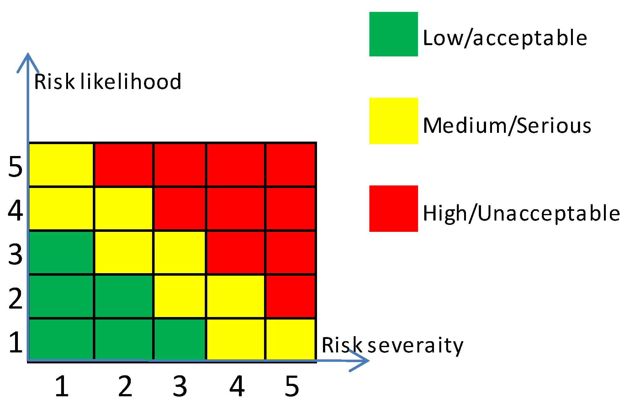
When a risk is classified as unacceptable/high risk, then one or more actions can be initiated for mitigation: control, eliminate, suppress or shift operation. Awati [32] identified violation of weak consistency condition in typical risk matrix based quantification and derived surprising consequences. Definition for Cox’s weak consistency is given below:
“A risk matrix with more than one ’color’ (level of risk priority) for its cells satisfies weak consistency with a quantitative risk interpretation if points in its top risk category (red) represent higher quantitative risks than points in its bottom category (green)” [32]. As a result, to satisfy weak consistency condition, risk matrix shall have at least three colors, as shown in Figure 2.
3. Problem Formulation
For underground risk analysis and assessment, we need to collect certain parameters of interest via sensors deployed at selected locations. Risk at any location and at any point in time depends on various associated factors, e.g., ground status, pipeline leakage, etc. These individual risk factors are referred to risk contributing factors (RCFs) here and denoted as . Each RCF has its contribution towards final risk index (FRI) at that particular location. We can express set of risk contributing factors as
For the sake of generality, we assume that m is the total number of RCFs. The risk index value for individual factor is expressed as and is calculated by fusion and aggregation of relevant sensor data after necessary processing.
In the real world, we cannot have sensors at every location; rather sensors are deployed at selected locations. Assume we have n selected locations in our area of interest, i.e., . We are interested in collecting information of about each for selected locations where value of each RCF is calculated by fusion and aggregation of various related sensors data, e.g., water supply pipeline leakage is calculated by fusing camera sensor data with water leak sensors along with flow and pressure sensors.
For the sake of simplicity, we express set of sensors required for estimation of RCF as . As we are considering m RCFs, therefore, at each selected location, we can have m different set of sensors, i.e., collecting information about every individual RCF. Thus, we need at most set of sensors in our area of interest. Each set of sensor gives us reading of a particular parameter on a selected location at particular time t expressed as . Sensor reading defines risk probability at particular location where impact of the risk is estimated by experts depending upon the location sensitivity.
Risk at any location and at any point in time depends on various associated RCF, e.g., ground status, pipeline leakage, etc., contributing towards the final risk index at that particular location. Thus, first we need to estimate risk index value for individual RCF at every selected location.
As mentioned previously, we assume m risk contributing factors (RCF) where risk index of factor at time t at location , i.e., depends on two main factors: (a) risk probability; and (b) risk severity. Mathematically, we can express it as below
In Equation (3), H is used to express an unknown function (because the actual relationship is unknown) taking two parameters, i.e., and , to compute . Here, is the risk probability calculated from sensors readings for factor at time t and is the impact severity of the risk factor at location . Risk probability of factor depends on the sensors reading at time t deployed at , i.e.,
In other words, risk probability of risk contributing factor depends on the sensor reading installed for that purpose. Various sensor readings are considered for concluding risk index of a particular risk contributing factor and individual sensors reading can be combined in several ways, for instance simple or weighted averaging scheme. Actual sensors reading and experts knowledge will be required to formulate the relationship among sensors readings and corresponding risk index value.
Risk severity of factor is a constant value depending upon the sensitivity and significance of the risk location, i.e.,
Equation (5) is a general equation for expressing risk severity of risk contributing factor and the equation shows that it only depends on the location sensitivity and significance which is to be determined by experts by visiting and inspecting the site. Risk severity of a location will be high if more damage to human lives and properties can occur in the case of collapse and vice versa.
After calculating individual risk for every parameter, we can now express final risk index on location at time t, i.e., as below.
In Equation (6), F is used to express an unknown function (because the actual relationship is unknown) taking risk index values of all m individual risk contributing factors as input to estimate the final risk index at given location. Here, is the risk index of factor at time t and location .
4. Approximation Schemes for Underground Risk Index
In our general formulation, we have two unknown functions given in Equations (3) and (6), respectively. In reality, these functions can be a very complex but, here, we try to find its approximation using three techniques: (a) linear approximation; (b) hierarchical fuzzy inference system based approximation; anf (c) hybrid approach based approximation. Next, we present brief description of these techniques.
4.1. Linear Approximation
First, we assume linear approximation for the unknown function in Equation (3) as below
where and are the weight assigned to risk probability and risk severity, respectively, such that . is the risk probability calculated from sensors readings for factor at time t and is the impact severity of the risk factor at location . After calculating individual risk for every parameter, we can now express a linear approximation for the final risk index on location at time t, i.e., given in Equation (6) as below.
where is contribution coefficient of factor towards final risk index and its values can be determined using multiple linear regression analysis.
4.2. Hierarchical Fuzzy Inference System based Approximation
This is a novel idea where related inputs are combined by various FIS systems in a tree-like structure to produce output. The hierarchical structure is a not strict tree because one input can serve as input to more than one parent nodes. Leaf nodes are used to express input variables in our system. Every internal node is an FIS system taking input from its child nodes and producing output for upper nodes. Output of root node is final outcome of hierarchical fuzzy inference system. We can have different possible formation for the hierarchical structure depending upon input-output relevancy, each forming a separate Model.
4.2.1. General Hierarchical Fuzzy Inference System
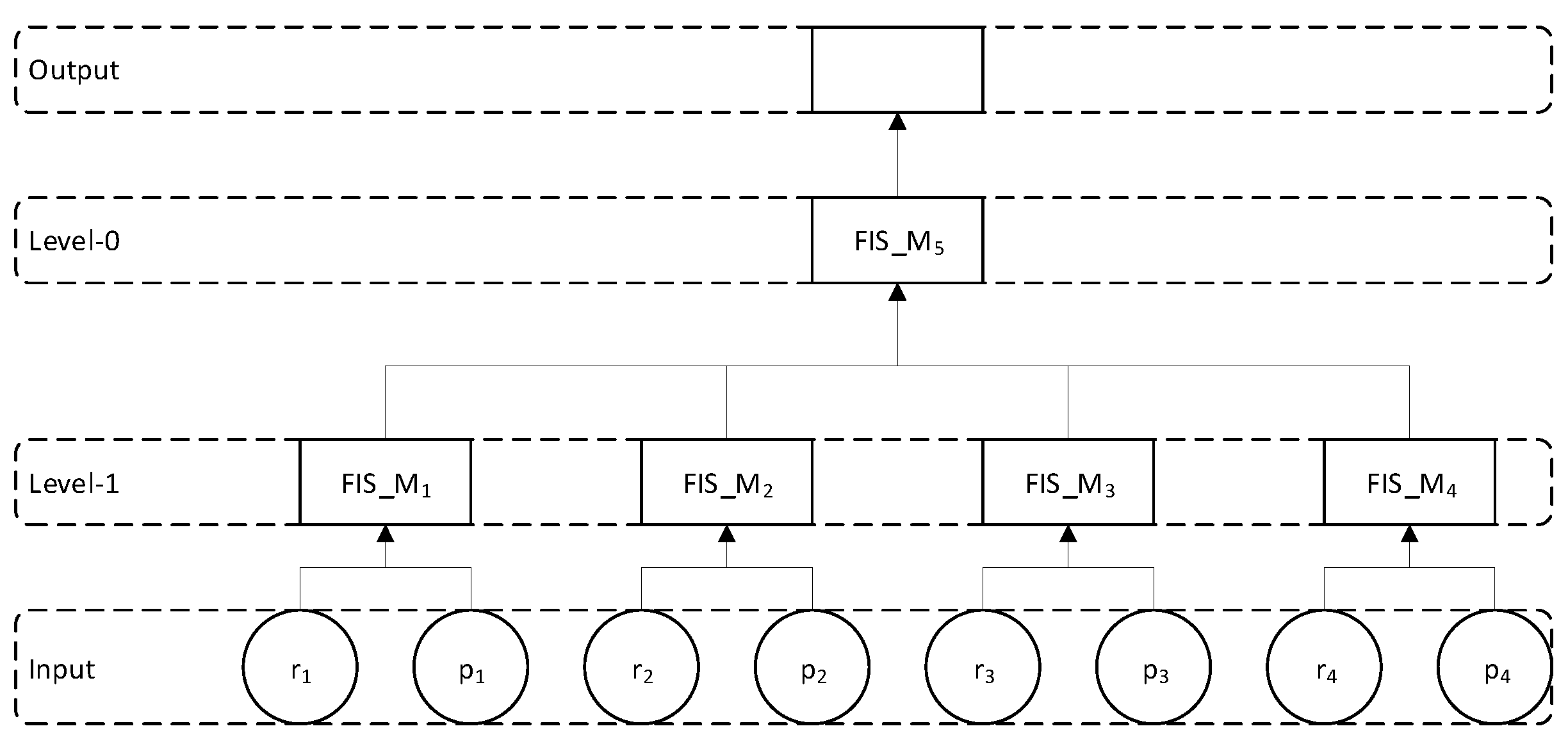
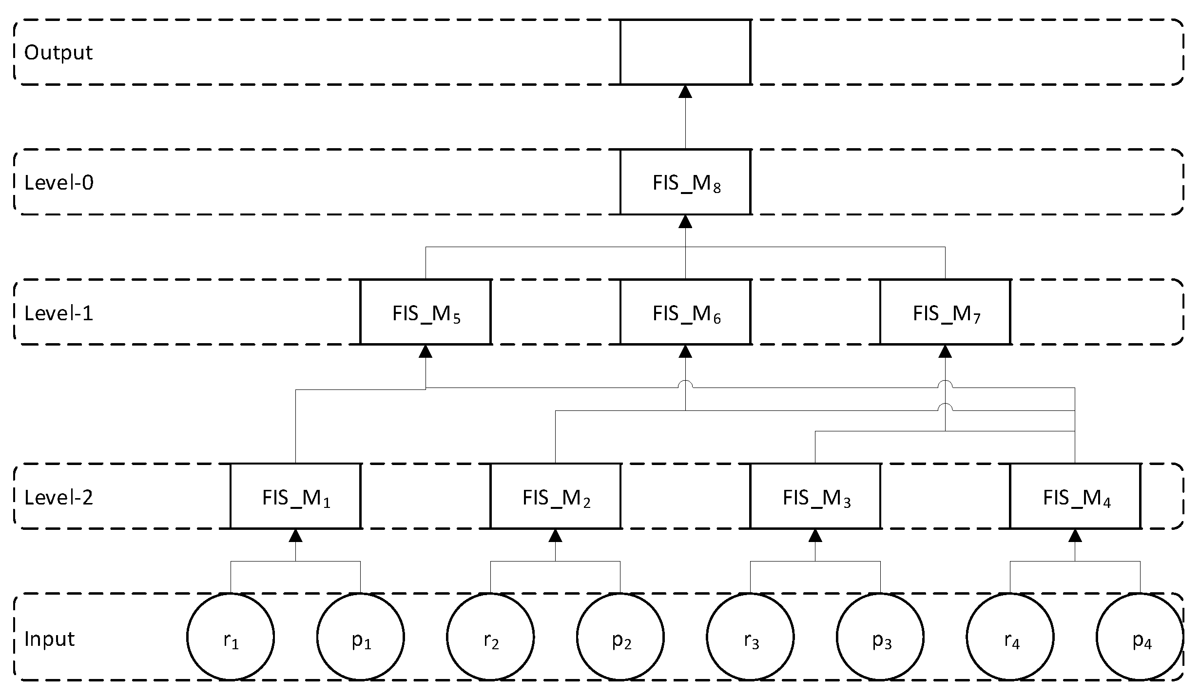
Figure 3 shows the general model for hierarchical fuzzy inference system. Depending on the number of inputs and its types, we can define and combine FIS system at various layers. In this example, we have seven input variables. Related variables are given to the FIS system at bottom Level 2. Output of FIS system at Level 2 is then given to FIS system at Level-1. Finally, at Level 0, we combine the output of FIS at Level 1 and Level 2. Same variables can be given as input to different FIS system if they are contributing to multiple fuzzy systems.
4.2.2. Approximation using Hierarchical Fuzzy Inference System
At the core of Hierarchical Fuzzy Inference System (FIS), we have several basic fuzzy inference systems connected together in a tree-like structure. Related inputs are fed to bottom layer FIS and its output is given to intermediate layer FIS. Finally, root nodes generates the system overall output. For example, in Figure 3, is a basic FIS taking and as input and generate output as . Different fuzzy inference system models can be used but we consider using Mamdani-type fuzzy inference system in this paper [33]. is then given as input to and so on. The final output of this hierarchical FIS system is which is calculated at top layer (Level 0). Output of Hierarchical FIS is obtained from repeated evaluation of all basic FIS, starting from the bottom layer and working upward to the root node. For the sample Hierarchical Model given in Figure 3, we have the following evaluations
i.e., in takes and as input and generate output as . is then given as input to and so on. The following evaluations are performed at intermediate layers.
where is the resultant output of the hierarchical FIS which is calculated at top layer, as shown in Figure 3.
4.3. Hybrid Approach Based Approximation
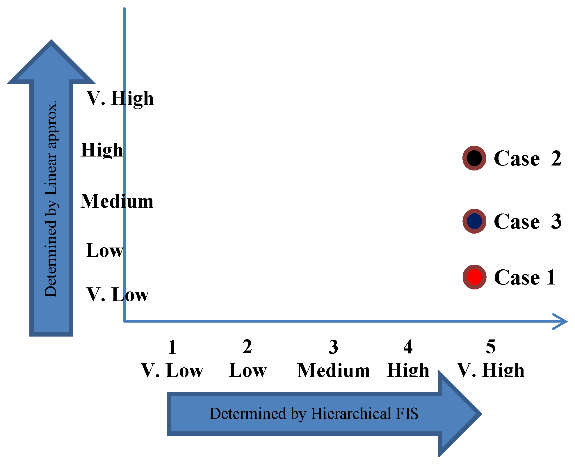
Hybrid approach is a combination of both linear approximation and hierarchical FIS system to capture teh strength of both and overcome their limitations. Here, final risk index is expressed as a point on 2D plot, as shown in Figure 4.
To map any risk index on this plot, we need its two coordinates, i.e., x and y. As shown in Figure 4, x-coordinate is determined by hierarchical FIS, whereas y-coordinate is determined by linear approximation. Thus, for risk information of a given location, we first apply hierarchical FIS approximation method to get x-coordinate of the risk point. Then, linear approximation model is applied on the same data values to obtain y-coordinate of the risk point. Afterwards, we can easily map the given risk information on the plot to determine its severity. Color coding used in Figure 2 also helps in improved visual representation of risk index information over map using heat mapping.
The bottom left corner is the safest situation and top right corner is the riskiest situation. Gradual increase along y-axis values can be observed while moving from left to right along x-axis. Hierarchical FIS tends to find final risk index by giving more preference to maximum risk index. If maximum risk index among all factors is low on x-axis, then linear approximated risk index cannot be more than low along y-axis. This is why, when maximum risk index along x-axis increases, possible average risk index also grows along y-axis.
For numerical computation and comparison, we can quantify the risk point on hybrid map into a single risk index value, as shown in Figure 5. Final risk values on hybrid map ranges from [0, 15) where 0 signifies most safe situation and 14.99 implies the extremely risky condition.
Every box is labeled with a numeric value inside showing the range of risk indexes for the corresponding point of mapping, e.g., the box for (medium, low) labeled as 4 covers the range of risk indexes from [4, 5), i.e., 4.0 is the bottom line and 4.99 for the top line.
5. Experimental Design
For experimental purposes, we restrict the set of risk contributing factors to four elements, i.e.,
where express water supply risk index, express sewerage line risk index, express metro structure risk index, and express ground state risk index. For every risk contributing factor, we have a corresponding risk probability and impact severance denoted as and , respectively.
5.1. Linear Approximation
Risk index of individual contributing factors on location at time t becomes
These experiments are conducted by assuming and . Total risk index can be calculated by linear approximation as below
Experiments are conducted for estimation of values using multiple linear regression analysis.
5.2. Hierarchical Fuzzy Inference System based Approximation
As stated earlier, we can combine the given input in many different ways to form the hierarchical structure named as model. For these experiments, we consider two models, as shown in Figure 6 and Figure 7.
In Model 2, risk index of selected contributing factors is calculated using risk probability and risk severity of each factor via basic FIS at Level 2. Next, ground state risk index is combined with the three other risk factors to get their effective risk index at Level 1. Finally, effective risk index of the three factors is combined at Level 0 to produce overall risk index for the given location.
Rules definition for Hierarchical Fuzzy Inference System
We have four risk contributing factors and their respective risk index is expressed as to . We need a single risk index value for a given location that is somehow representative of all four risk index values. In Hierarchical FIS, we selected two different possible formations for the hierarchical structure for experimental purposes, i.e., Model 1 and Model 2. To define rules for our hierarchical FIS, we tried two different strategies, i.e., maximum based and average based. For the sake of illustration, we consider five different linguistic variables for individual risk contributing factor, i.e., very low, low, medium, high, abd very high. Numeric values assigned to each risk label are shown in Table 1. Rules definition as per both schemes are demonstrated in Table 2 for three sample rules representing three different cases. These three cases were carefully selected for two reasons. (a) To illustrate the working of the two schemes used for rules definition in fuzzy inference system, i.e., maximum based scheme and average based scheme. Different values are assigned to individual risk contributing factors M1 to M4 for the three selected cases and the corresponding output calculation is shown in the Table 2 using the two schemes. (b) To highlight a weakness in the two selected schemes for rules definition using these three sample cases (briefly discussed in Section 5.3). Case 2 and Case 3 are quite different but the resultant output is almost same for both maximum and average based schemes. In other words, maximum based scheme treat all three cases as the same (critical) and fails to capture the difference among the three cases. Average based scheme treats Case 2 and Case 3 almost the same, which is not true in reality.
5.3. Hybrid Approach Based Approximation
This is a combination of both linear approximation and hierarchical FIS system, which captures the strengths of both and overcomes their limitations. We can see in Table 2 that three sample cases are different but not reported appropriately by average based or maximum based schemes.
- For Case 1, average based scheme result is Low, thus ignoring M4, which may be critical.
- Case 2 and Case 3 are treated as the same by both schemes which is not true.
Thus, for any given data values of risk index, we first apply hierarchical FIS approximation method to get x-coordinate of the risk point. Then, linear approximation model is applied on the same data values to obtain y-coordinate of the risk point. It can be seen in Figure 8 that hybrid approach accurately reports the cases while maintaining their differences. As per hybrid approach, all three cases are critical but Case 1 is less critical, having one critical risk index and low y-coordinate. Case 2 is positioned near the top right corner, showing that it is the most critical situation.
6. Implementation of Approximation Schemes for Underground Risk Index
6.1. Linear Approximation
We have risk index of individual contributing factors on location . Final risk index can be calculated by linear approximation as below
Using multiple linear regression analysis, estimated values for are as follows: , , , , and . Putting these values into Equation (18), we get
Thus, we calculate final risk index as a linear combination of the four risk contributing factors by linear approximation scheme.
6.2. Hierarchical Fuzzy Inference System Based Approximation
We implemented the two selected models as shown in Figure 6 and Figure 7 in MATLAB for evaluating results of hierarchical FIS. For all fuzzy inference sub-systems, we used the Mamdani-type fuzzy inference system which follows a four-step process to compute the crisp output from given inputs. A very useful tutorial on the internal working of Mamdani-type fuzzy inference system can be found in [34]. Table 3 presents the settings used in each step of Mamdani-type fuzzy inference system.
Range of risk index values of selected risk contributing factors is [0, 10] which is covered by five overlapping triangular membership functions with details given in Table 4. The same scheme is also used for output, i.e., final risk index.
Every model is separately evaluated twice: (a) average based scheme for rule definition; and (b) maximum based scheme for rule definition. Illustration of both schemes is given in Table 2 for three sample rules. After fuzzification process, antecedent of each rule is computed by selecting minimum (or maximum) value if the inputs of the rule are combined via AND (or OR) operation. Minimum operation is used in implication step to compute consequent of the rule from given antecedent values. In the third step, aggregation is performed using maximum operation to combine resultant consequent of all rules. Finally, centroid method is applied to compute crisp output in the last defuzzification step.
6.3. Hybrid Approach Based Approximation
Hybrid approach based approximation is similar to scatter plotting of risk index calculated by two different schemes on x–y plane. We choose best Hierarchical FIS results value for x-axis and linear approximation results are taken as its y-axis. Higher values along y-axis show that average value is high which means more factors are critical and vice versa. Higher values along x-axis show that final risk index is high, as reported by hierarchical FIS. Suppose we have risk index of individual contributing factors on location then,
and
Next, for x- and y-coordinate of the point on x–y plane expressing hybrid risk index, we perform scaling on and as below.
We divide and by 10 as both maximum value as 10. Similarly, we multiply the result with 5 because maximum value for x- and y-coordinate on hybrid risk point is 5. For quantification of hybrid risk point from x–y plane into a single final risk index on scale 0 to 10, we use the following formula.
where the final risk index, i.e., FinalRiskIndex computed in Equation (23) through hybrid approximation scheme is the same as the final risk index calculated in Equation (6).
7. Results and Discussion
For experimental purposes, we used synthetic data to evaluate accuracy and effectiveness of proposed models. Various input parameters are considered to estimate values of the four risk contributing factors for every location which serve as input data to our system. Length, depth, size and age (years of burial), leakage probability and pipeline ductability are the input parameters for water supply risk index () and sewerage line risk index (); age and degree of peripheral depression for metro structure risk index (); and granularity, compaction and ground water level for ground state risk index (). We have considered 100 different locations and values for each parameter are carefully selected from a valid range as given in Table 5 to have maximum diversity in the final dataset. Each parameter value is then scaled in range [0, 10]. Risk index for each factor is calculated by taking simple average of three schemes, i.e., simple average, weighted average and maximum based scheme. Finally, risk index values are also scaled in range [0, 10] where zero mean no risk and 10 means very high risk. To get estimated final risk index, data generated are first labeled for various selected parameters by assigning a descriptive label to express the corresponding parameters in a formal language such as very low, low, medium, high and very high. Descriptive data for each location with labeled parameters are then provided to three experts and they were asked to provide expected risk index for given locations based on their experience and expertise. Average values were taken to get estimated final risk for corresponding locations which is then used for comparative analysis with proposed method.
First, we present results of linear approximation scheme. In this method, we estimate weights for all risk contributing factors using multiple linear regression analysis. As shown in Figure 9, linear approximation results match fairly well but are not fully aligned with estimated risk index as desired. This shows that final risk index cannot be estimated from simple linear combination of risk contributing factors.
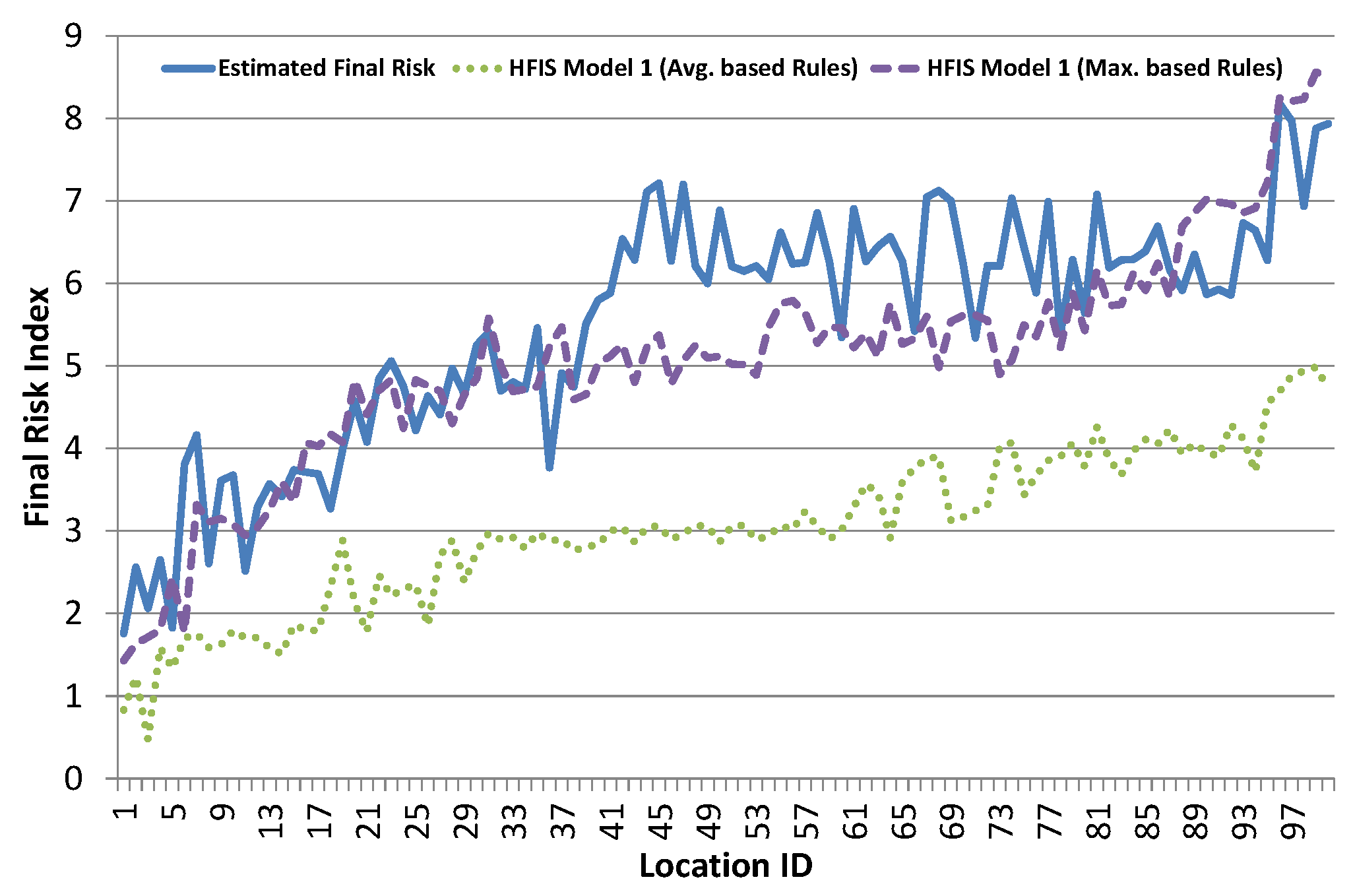
Next, we evaluate hierarchical FIS models. As discussed earlier, we have selected two different models for evaluating results of hierarchical FIS, as shown in Figure 6 and Figure 7. Every model is separately evaluated for rules defined via both average based and maximum based schemes. Result of Basic Hierarchical FIS Model 1 is shown in Figure 10. Average based rule definition scheme results are not good, as they lag far behind the estimated risk index. This shows that average based rules definition scheme suppresses the final risk index and fails to capture desired results. Maximum based rule definition scheme results are much better for all locations except for the middle part.
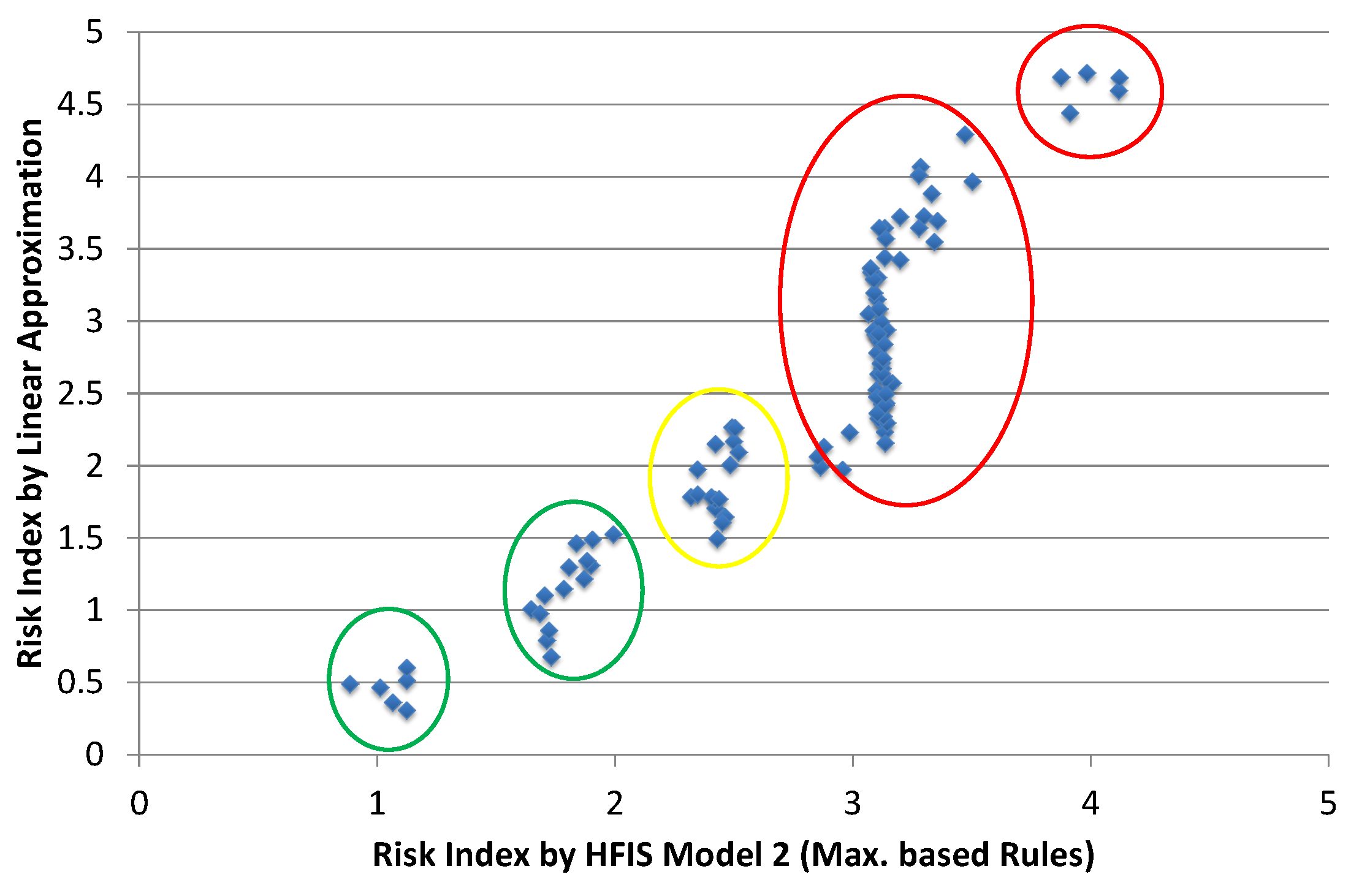
Result of Integrated Hierarchical FIS Model 2 is shown in Figure 11. As in Model 1, average based rule definition scheme results are even worse in Model 2 as intermediate layers further suppress the final risk index and fail to produce desired output. Maximum based rule definition scheme results are much better and very close to estimated risk index. It seems better than Model 1 maximum based scheme results. This shows that intermediate layer in Model 2 helps in revealing the hidden structure among risk contributing factors.
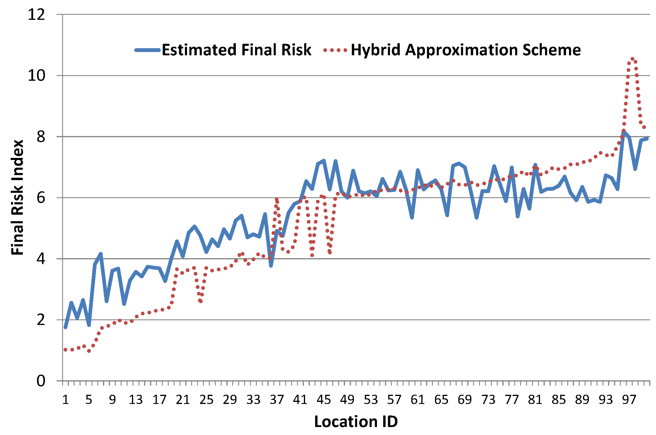
Hybrid approach estimation results for final risk index are shown in Figure 12. These results show that hybrid scheme fails to accurately estimate final risk index. However, scatter plot of hybrid scheme carries some interesting and detailed information, as shown in Figure 13. It somehow performs automatic clustering and five different clusters are indicated in Figure 13. Movement along x-axis shows increase in risk index due to any single factor. However, vertical rise along y-axis shows that risk index of contributing factors is growing, which results in increase average risk index. Location plotted in left bottom area has the lowest risk (highlighted in green circle). In the center, there are few locations with medium risk. Horizontal part in estimated risk index, i.e., from location ID 50 to 90, is reflected in the biggest cluster having vertical tendency. Small cluster at the top right corner shows the most critical locations.
Comparison results of risk index approximation schemes for four statistical measures are given in Table 6. Average based rule definition results for both Hierarchical FIS system (i.e., Model 1 and Model 2) are worse than simple linear approximation. Maximum based scheme results for Model 2 have the best correlation (+0.917) with estimated risk index. Furthermore, it can also be seen that Model 2 (maximum based) results are best in all statistical measures which proves that: (a) layering structure of Model 2 accurately captures the relationship among risk contributing factors; and (b) maximum based rule definition scheme allows the model to produce better results than average based scheme.
8. Conclusions and Future Work
In this paper, we have presented analytical modeling for underground risk assessment in smart cities. For evaluation purposes, we have selected three different schemes: (a) linear approximation schemes, in which we tried to establish a linear relationship between risk contributing factors using multiple linear regression analysis, however its results were not promising, indicating that linear relationship do not exist among risk contributing factors; (b) hierarchical fuzzy logic based schemes were tested using two different models, i.e., simple and integrated with two different schemes for rules definition; and (c) hybrid approach is a combination of both linear approximation and hierarchical FIS system to capture the strengths of both as well as overcome their limitations. Comparative analysis of the statistical results shows that integrated hierarchical Model 2 with maximum based scheme for rules definition produce the best results. Estimation results based on hybrid approach fail to accurately estimate final risk index. However, hybrid scheme reveals some interesting and detailed information, i.e., it somehow performs automatic clustering and five different clusters are indicated based on risk index. Thus, hybrid approach is useful for segregating locations based on their estimated risk index. This is also helpful in preparing priority list for maintenance teams to perform necessary corrective measure on urgent basis for most critical locations. These initial results give us confidence to further explore and extend this work by performing experiments on real data. We will also explore other advanced schemes for risk assessment and approximation.
Author Contributions
I.U. proposed the analytical model for underground risk assessment, conducted the experiments and wrote the manuscript. M.F. assisted in performing the comparative analysis and results collection. D.K. conceived the overall idea of underground risk assessment in smart cities and supervised this work. All authors contributed to this paper.
Acknowledgments
This research was supported by the MSIT(Ministry of Science and ICT), Korea, under the ITRC(Information Technology Research Center) support program(IITP-2017-2016-0-00313) supervised by the IITP(Institute for Information & communications Technology Promotion) and this research(paper) was performed for the Development of Radar Payload Technologies for Compact Satellite in Korea Aerospace Research Institute, funded by the Ministry of Science and ICT. Any correspondence related to this paper should be addressed to DoHyeun Kim; [email protected].
Conflicts of Interest
The authors declare no conflict of interest.
References
- De Stefano, A. On-line monitoring and resilient design for a longer construction life. In Proceedings of the 46th ESReDA Seminar, Turin, Italy, 29–30 May 2014. [Google Scholar]
- Ortiz, P.; Antunez, V.; Martín, J.M.; Ortiz, R.; Vázquez, M.A.; Galán, E. Approach to environmental risk analysis for the main monuments in a historical city. J. Cult. Heritage 2014, 15, 432–440. [Google Scholar] [CrossRef]
- Designing for Disaster. 2010. Available online: http://www.design4disaster.org/ (accessed on 12 February 2018).
- Khan, M.S.; Park, D.H.; Kim, D. System Modelling Approach Based on Data Acquisition and Analysis for Underground Facility Surveillance. Int. J. Smart Home 2016, 10, 93–102. [Google Scholar] [CrossRef]
- Choi, H.H.; Cho, H.N.; Seo, J. Risk assessment methodology for underground construction projects. J. Constr. Eng. Manag. 2004, 130, 258–272. [Google Scholar] [CrossRef]
- Kim, S.; Choi, D.; Ahn, C. Tunnel design underneath the operating runway of Incheon airport. In Geotechnical Aspects of Underground Construction in Soft Ground; Korean Geotechnical Society: Seoul, Korea, 2014; pp. 43–48. [Google Scholar]
- Sturk, R.; Olsson, L.; Johansson, J. Risk and decision analysis for large underground projects, as applied to the Stockholm ring road tunnels. Tunn. Undergr. Space Technol. 1996, 11, 157–164. [Google Scholar] [CrossRef]
- Ghosh, S.; Jintanapakanont, J. Identifying and assessing the critical risk factors in an underground rail project in Thailand: A factor analysis approach. Int. J. Proj. Manag. 2004, 22, 633–643. [Google Scholar] [CrossRef]
- Mayer, P.; Corriols, A.; Hartkorn, P.; Messing, M. Risk assessment for infrastructures of urban areas. Undergr. Infrastruct. Urban Areas 2014, 3, 125. [Google Scholar]
- Lej, K. The technical and economic conditions for the construction of the central section of metro line II in Warsaw. Undergr. Infrastruct. Urban Areas 2014, 3, 85. [Google Scholar]
- Liu, Z.; Kleiner, Y. State of the art review of inspection technologies for condition assessment of water pipes. Measurement 2013, 46, 1–15. [Google Scholar] [CrossRef] [Green Version]
- Fletcher, R.; Chandrasekaran, M. SmartBall™: A New Approach in Pipeline Leak Detection. In 2008 7th International Pipeline Conference; American Society of Mechanical Engineers: New York, NY, USA, 2008; pp. 117–133. [Google Scholar]
- Kong, X.; Tang, X.; Humphrey, D.; Mergelas, B.; Mascarenhas, R. Live inspection of large diameter PCCP using a free-swimming tool. In Pipelines 2010: Climbing New Peaks to Infrastructure Reliability: Renew, Rehab, and Reinvest; American Society of Civil Engineers: Reston, VA, USA, 2010; pp. 1006–1015. [Google Scholar]
- Kuttisseril, J.; Kuang, K. Development of a low-cost image processing technique for crack detection for structural health monitoring. In 3rd ASEAN Australian Engineering Congress (AAEC 2015): Australian Engineering Congress on Innovative Technologies for Sustainable Development and Renewable Energy; Engineers Australia: Barton, Australia, 2015; p. 55. [Google Scholar]
- Sankarasrinivasan, S.; Balasubramanian, E.; Karthik, K.; Chandrasekar, U.; Gupta, R. Health monitoring of civil structures with integrated UAV and image processing system. Procedia Comput. Sci. 2015, 54, 508–515. [Google Scholar] [CrossRef]
- Sun, M.H.; Zhao, Y.X.; Jiang, W.; Feng, T.T. A scheme for excavation displacement monitoring based on image processing. Appl. Mech. Mater. 2012, 226, 1923–1926. [Google Scholar] [CrossRef]
- Jahanshahi, M.R.; Masri, S.F. Adaptive vision-based crack detection using 3D scene reconstruction for condition assessment of structures. Autom. Constr. 2012, 22, 567–576. [Google Scholar] [CrossRef]
- Qi, D.; Liu, Y.; Wu, X.; Zhang, Z. An algorithm to detect the crack in the tunnel based on the image processing. In Proceedings of the 2014 Tenth International Conference on Intelligent Information Hiding and Multimedia Signal Processing (IIH-MSP), Kitakyushu, Japan, 27–29 August 2014; pp. 860–863. [Google Scholar]
- Alam, M.A.; Ali, M.N.; Syed, M.A.A.A.; Sorif, N.; Rahaman, M.A. An algorithm to detect and identify defects of industrial pipes using image processing. In Proceedings of the 2014 8th International Conference on Software, Knowledge, Information Management and Applications (SKIMA), Dhaka, Bangladesh, 18–20 December 2014; pp. 1–6. [Google Scholar]
- Kleta, H.; Heyduk, A. Image processing and analysis as a diagnostic tool for an underground infrastructure technical condition monitoring. Undergr. Infrastr. Urban Areas 2014, 3, 39. [Google Scholar]
- Knudsen, O.O.; Giertsen, E.; Schjolberg-Henriksen, P.; Ostby, E.; Grythe, K.; Oldervoll, F. SmartPipe: Self Diagnostic Pipelines and Risers. In Proceedings of the ASME 2007 26th International Conference on Offshore Mechanics and Arctic Engineering, San Diego, CA, USA, 10–15 June 2007; pp. 161–166. [Google Scholar]
- Schempf, H. In-Pipe-Assessment Robot Platforms-Phase I-State-Ofthe-Art Review; Report to National Energy Technology Laboratory REP-GOV-DOE-20041102; CMU: Pittsburgh, PA, USA, 2004. [Google Scholar]
- Datta, K.; Fraser, D.R. A corrosion risk assessment model for underground piping. In Proceedings of the 2009 Annual Reliability and Maintainability Symposium, Fort Worth, TX, USA, 26–29 January 2009; pp. 263–267. [Google Scholar]
- Romanoff, M. Underground corrosion, National Bureau of Standards Circular 579; US Government Printing Office: Washington, DC, USA, 1957; Volume 25.
- Rossum, J.R. Prediction of pitting rates in ferrous metals from soil parameters. J. Am. Water Works Assoc. 1969, 61, 305–310. [Google Scholar] [CrossRef]
- Kumar, A.; Meronyk, E.; Segan, E. Development of Concepts for Corrosion Assessment and Evaluation of Underground Pipelines; Technical Report; US Army Construction Engineering Research Laboratory (ARMY): Champaign, IL, USA, 1984. [Google Scholar]
- Rajani, B. Investigation of Grey Cast Iron Water Mains to Develop A Methodology for Estimating Service Life; American Water Works Association: Denver, CO, USA, 2000. [Google Scholar]
- Sheikh, A.; Boah, J.; Hansen, D. Statistical modeling of pitting corrosion and pipeline reliability. Corrosion 1990, 46, 190–197. [Google Scholar] [CrossRef]
- Ericson, C.A. Fault tree analysis. Hazard Anal. Tech. Syst. Saf. Wiley Online Library 2005, 183–221. [Google Scholar]
- Avestedt, L. Comparison of Risk Assessments for Underground Construction Projects A Study about Distinctions and Common Features and Suggestions for Improvements. Master’s Thesis, Royal Institute of Technology, Stockholm, Sweden, 2012. [Google Scholar]
- Dumbravă, V.; Iacob, V.S. Using probability—Impact matrix in analysis and risk assessment projects. J. Knowl. Manag. Econ. Inf. Technol. 2013, 42, 76–96. [Google Scholar]
- Awati, K. Cox’s Risk Matrix Theorem and Its Implications for Project Risk Management. 2011. Available online: https://eight2late.wordpress.com/2009/07/01/cox%E2%80%99s-risk-matrix-theorem-and-its-implications-for-project-risk-management/ (accessed on 07 January 2018).
- Mamdani, E.H.; Assilian, S. An experiment in linguistic synthesis with a fuzzy logic controller. Int. J. Man-Mach. Stud. 1975, 7, 1–13. [Google Scholar] [CrossRef]
- Alonso, S.K. eMathTeacher: Mamdani’s Fuzzy Inference Method. 2014. Available online: http://www.dma.fi.upm.es/recursos/aplicaciones/logica_borrosa/web/fuzzy_inferencia/mamdani_en.htm (accessed on 13 January 2018).
Figure 1.
Conceptual design of underground risk assessment system.

Figure 2.
Typical risk matrix.

Figure 3.
General Hierarchical Fuzzy Inference System.
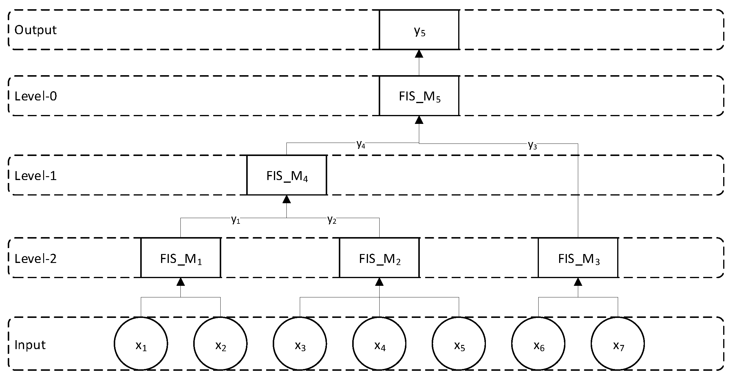
Figure 4.
Risk index mapping using hybrid approach.
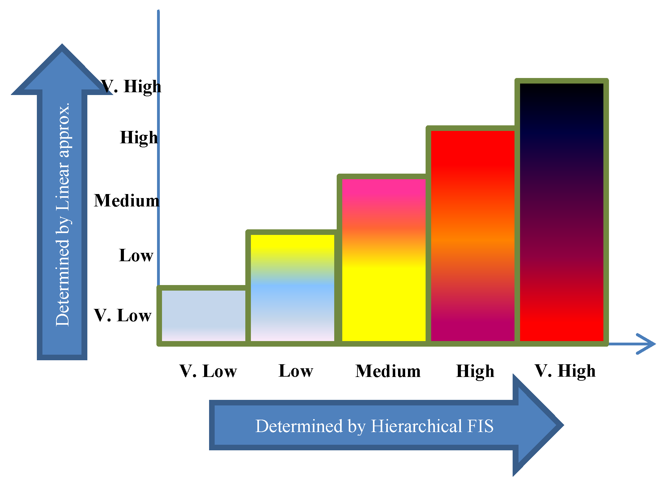
Figure 5.
Quantifying risk index using hybrid approach.
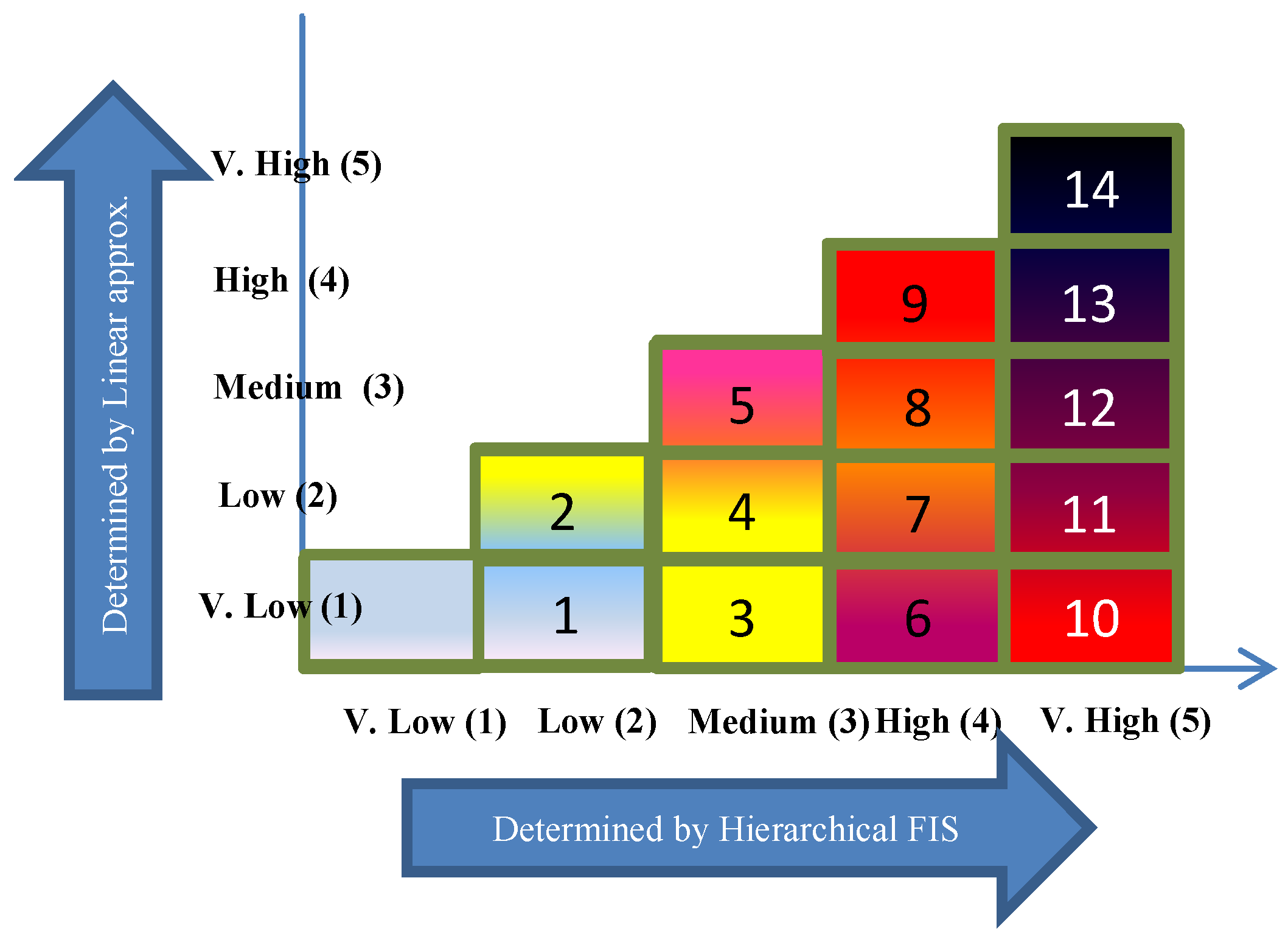
Figure 6.
Model 1: basic hierarchical FIS.

Figure 7.
Model 2: integrated hierarchical FIS.

Figure 8.
Risk mapping of three sample cases using hybrid approach.

Figure 9.
Final risk index results based on linear approximation.
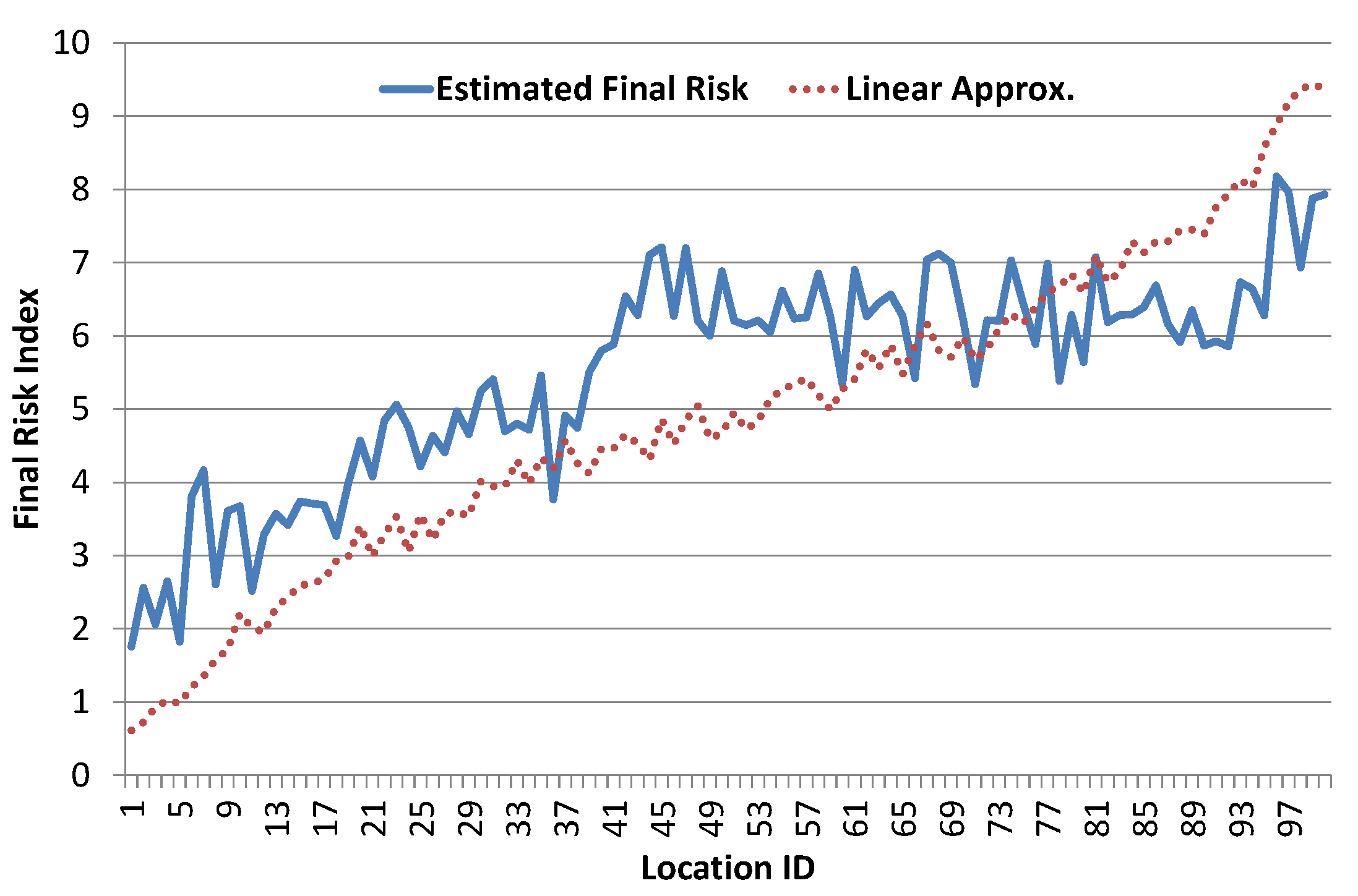
Figure 10.
Results of basic hierarchical FIS Model 1.

Figure 11.
Results of integrated hierarchical FIS Model 2.
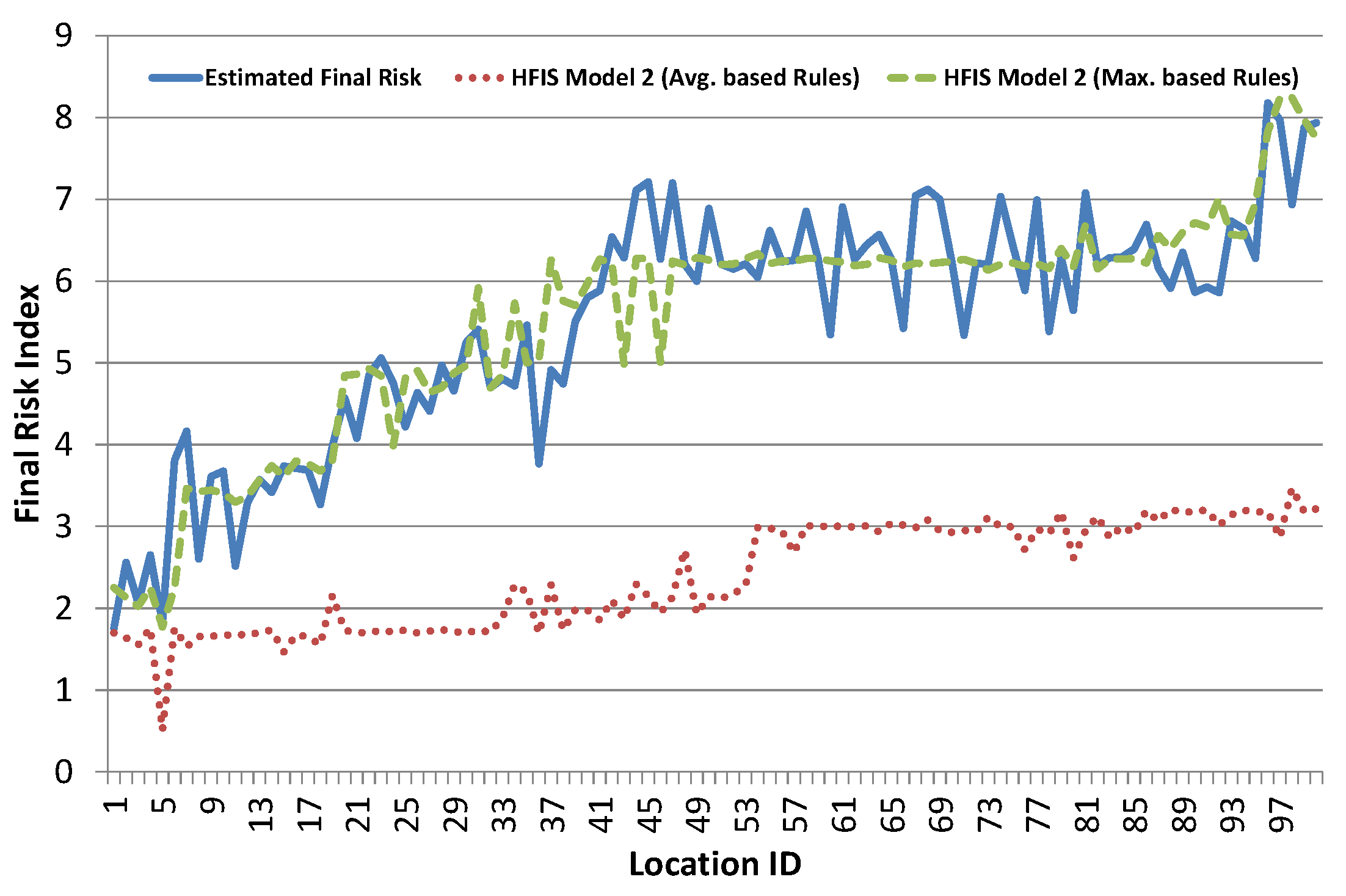
Figure 12.
Final risk index results using hybrid approach.

Figure 13.
Clustering of locations based on risk index using hybrid approach.


Table 1.
Numeric values for corresponding linguistic variables.
| Label | Very Low | Low | Medium | High | Very High |
|---|---|---|---|---|---|
| Value | 1 | 2 | 3 | 4 | 5 |
Table 2.
Example cases for illustration of rules definition using average and maximum based schemes.
Table 2.
Example cases for illustration of rules definition using average and maximum based schemes.
| S. No. | Input | Output | ||||
|---|---|---|---|---|---|---|
| M1 | M2 | M3 | M4 | Max-Based | Avg.-Based | |
| Case 1 | V.Low | V.Low | V.Low | V.High | V.High | Low |
| 1 | 1 | 1 | 5 | 5 | (1 + 1 + 1 + 5)/4 = 2 | |
| Case 2 | High | High | High | V.High | V.High | High |
| 4 | 4 | 4 | 5 | 5 | (4 + 4 + 4 + 5)/4 = 4.25 | |
| Case 3 | - | - | Medium | V.High | V.High | High |
| 3 | 5 | 5 | (3 + 5)/2 = 4 | |||
Table 3.
FIS Components Configuration.
| FIS Component | Membership Function | Fuzzification | Implication | Aggregation | Defuzzification |
|---|---|---|---|---|---|
| Method used | Triangular | Min for AND Max for OR | Min | Max | Centroid |
Table 4.
Labels, ranges of input and output membership functions.
| Membership Function Name | Membership Function Labels | Range |
|---|---|---|
| Very Low | VL | (0.0 to 1.5) |
| Low | L | (0.5 to 4.0) |
| Medium | M | (3.0 to 7.0) |
| High | H | (6.0 to 9.5) |
| Very High | VH | (8.5 to 10) |
Table 5.
Selected parameters range and units for four risk contributing factors.
| Risk Contributing Factor | Parameter | Unit | Range |
|---|---|---|---|
| Water supply risk index (M1) | Length | [m] | (0–300) |
| Depth | [mm] | (0–2500) | |
| Years of burial | [year] | (0–30) | |
| Leakage probability | [%] | (0–100) | |
| Pipeline ductability | [cm] | (0–100) | |
| Sewerage line risk index (M2) | Length | [m] | (0–300) |
| Depth | [mm] | (0–2500) | |
| Years of burial | [year] | (0–30) | |
| Leakage probability | [%] | (0–100) | |
| Pipeline ductability | [cm] | (0–100) | |
| Metro structure risk index (M3) | Age | [year] | (0–30) |
| Degree of peripheral depression | [%] | (0–100) | |
| Ground state risk index (M4) | Granularity | [%] | (0–100) |
| Compaction | [%] | (0–100) | |
| Ground water level | [m] | (0–10) |
Table 6.
Statistical comparison of selected risk index approximation schemes.
| Statistical Measure | Linear Approximation | Basic Hierarchical FIS Model 1 | Integrated Hierarchical FIS Model 2 | ||
|---|---|---|---|---|---|
| Avg. based | maximum based | Avg. based | maximum based | ||
| Mean Absolute Deviation (MAD) | 1.16 | 2.46 | 0.73 | 3.1 | 0.43 |
| Mean Square Error (MSE) | 1.71 | 6.72 | 0.82 | 10.67 | 0.33 |
| Root Mean Square Error (RMSE) | 1.31 | 2.59 | 0.91 | 3.26 | 0.57 |
| Correlation Coefficient (R) | 0.77 | 0.85 | 0.83 | 0.77 | 0.91 |
© 2018 by the authors. Licensee MDPI, Basel, Switzerland. This article is an open access article distributed under the terms and conditions of the Creative Commons Attribution (CC BY) license (http://creativecommons.org/licenses/by/4.0/).
Share and Cite
MDPI and ACS Style
Ullah, I.; Fayaz, M.; Kim, D. Analytical Modeling for Underground Risk Assessment in Smart Cities. Appl. Sci. 2018, 8, 921. https://doi.org/10.3390/app8060921
AMA Style
Ullah I, Fayaz M, Kim D. Analytical Modeling for Underground Risk Assessment in Smart Cities. Applied Sciences. 2018; 8(6):921. https://doi.org/10.3390/app8060921
Chicago/Turabian StyleUllah, Israr, Muhammad Fayaz, and DoHyeun Kim. 2018. "Analytical Modeling for Underground Risk Assessment in Smart Cities" Applied Sciences 8, no. 6: 921. https://doi.org/10.3390/app8060921
Note that from the first issue of 2016, this journal uses article numbers instead of page numbers. See further details here.