Abstract
Although the policy-gradient methods for reinforcement learning have shown significant improvement in image captioning, how to achieve high performance during the reinforcement optimizing process is still not a simple task. There are at least two difficulties: (1) The large size of vocabulary leads to a large action space, which makes it difficult for the model to accurately predict the current word. (2) The large variance of gradient estimation in reinforcement learning usually causes severe instabilities in the training process. In this paper, we propose two innovations to boost the performance of self-critical sequence training (SCST). First, we modify the standard long short-term memory (LSTM)based decoder by introducing a gate function to reduce the search scope of the vocabulary for any given image, which is termed the word gate decoder. Second, instead of only considering current maximum actions greedily, we propose a stabilized gradient estimation method whose gradient variance is controlled by the difference between the sampling reward from the current model and the expectation of the historical reward. We conducted extensive experiments, and results showed that our method could accelerate the training process and increase the prediction accuracy. Our method was validated on MS COCO datasets and yielded state-of-the-art performance.
1. Introduction
Image captioning is the task of automatically describing an image with natural language. As shown in Figure 1, image caption methods usually follow the encoder–decoder paradigm. The process often includes two parts: a convolutional neural network (CNN) to encode an image into semantic features, and a recurrent neural network (RNN) to decode the input features into a text sequence word-by-word. At the training stage, the RNN is typically given the previous ground-truth word and trained to predict the next word with the cross-entropy loss as target function, while at test-time the model is expected to generate the entire sequence from scratch. This discrepancy between training and testing which is regarded as an exposure bias causes error accumulation during generation at test time. This will lead to suboptimality of the maximum likelihood training [1,2].
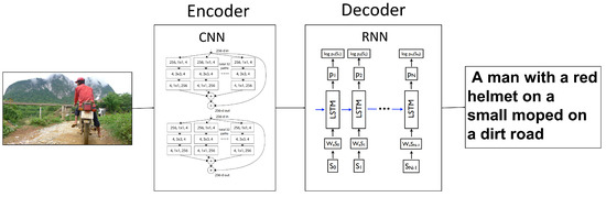
Figure 1.
Overview of the image caption model. It includes two parts: a convolutional neural network (CNN) to encode an image into semantic features, and a recurrent neural network (RNN) to decode the input features into a text sequence word-by-word. long-short term memory (LSTM) is a widely used decoder, because original RNN has vanishing and exploding gradients problems.
Recently, some reinforcement learning (RL)-based methods [1,3,4] have been proposed to tackle this problem. In these methods, the text generation is viewed as a stochastic procedure in which the word generation is modeled as action selection and the task-specific score (e.g., CIDEr [5] score) can be formulated as the reward directly. By using RL, the exposure bias problem can be addressed, and the non-differentiable task-specific metric can be directly optimized. However, it suffers from two significant issues. The first issue is that the image captioning has a high dimension of action space (e.g., token/word actions). It is challenging to learn an exact policy in such an action space. Besides, the high dimensionality of the sample space leads to high variance of the Monte Carlo estimates [6], which thus aggravates the instability of the RL training. Another issue is the high variance of the gradient estimation, which may cause the training to be unstable. Existing methods have attempted to reduce the variance via a learned baseline or a critic network [7] by training another network, which increased the difficulty of optimization. In order to avoid training a new network, self-critical sequence training (SCST) [4] was proposed. This model is based on the reward of the RL, which is obtained at the test inference time. However, the learned baseline is not a tight approximation of the expected reward signal. This also leads to high variance of the estimated gradient. In addition, we have found that the greedy method in SCST usually results in a higher reward than the multinomial sampling, and this is problematic since the baseline is too high for the agent to get positive feedback, and the training may get blocked.
To tackle the above two issues, we propose a boosted learning framework based on SCST with the following two innovations. First, we design a word-gated long short-term memory (LSTM) decoder to generate the output caption after encoding an input image with a deep CNN, in which the word gate function is used to predict the distribution of possible words regarding the input image. Specifically, the word gate is trained directly under the supervision of the words that appear in the ground-truth sentence. Our method draws inspiration from the observation that although the image captioning has large vocabulary, the actual quantity of valid words for a given image is relatively small. For example, given an image about the summer, the word “snow” is unlikely to be presented. From this viewpoint, the word gate function can significantly reduce the valid action space of the RL method, and further guide the output of the text generation model.
Secondly, for more stable gradient estimation, we give an improved version of SCST, called adaptive self-critical sequence training (ASCST), which brings a more approximate expected reward, and thus leads to easier optimization and better performance. The history reward information of the sample and greedy methods can tell approximately how wide the gap between the expected reward and the computed baseline is. By adaptively adjusting the greedily computed baseline with the history reward information of the sample and greedy methods, we can shrink the gap between the baseline and the expected reward, and thus significantly reduce the variance. We also introduce a novel control parameter to rescale the baseline adaptively with history reward information. Since natural learning progress moves from easy to hard, we introduce another parameter that gradually increases the baseline as the model converges. By adopting these two control parameters to the baseline, the performance of the agent can gradually ramp up and the training is stabilized.
The contributions of this paper are presented as follows:
- we introduce the word gate to dramatically reduce the valid action space of the text generation, which brings the reduced variance and easier learning.
- We present the adaptive SCST (ASCST), which incorporates two control parameters into the estimated baseline. We show that this simple yet novel approach significantly lowers the variance of the expected reward and gains improved stability and performance over the original SCST method.
- Experiments on MSCOCO dataset [8] show the outstanding performance of our method.
2. Related Work
2.1. Image Captioning
Inspired by the success of deep neural networks in neural machine translation, the encoder–decoder framework has been proposed for image captioning [9]. Vinyals et al. [9] first proposed an encoder–decoder framework which contained a CNN-based image encoder and an RNN-based sentence decoder, and was trained to maximize the log-likelihood. Various other approaches have been developed. Xu et al. [10] proposed a spatial mechanism to attend to different parts of the image dynamically. Authors in [11,12] integrated high-level attributes into the encoder–decoder framework by feeding the attribute features into RNNs. However, the attributes only concerned top-frequency words, which only account for about 10% of all the words in the vocabulary.
2.2. Image Captioning with Reinforcement Learning
Recently a few studies [1,3,4] have been proposed which used techniques from RL to address the exposure bias [1] and the non-differentiable task metric problems. However, compared to standard RL applications, image captioning has a much larger action space. The large action space will cause a high variance in gradient estimates in RL [6], which is proved to be the cause of unstable training. Variance reduction can often be achieved with a learned baseline or critic. Ranzato et al. [1] were the first to train the sequence model with policy gradient, and they used the RL algorithm [13] with a baseline estimated by a linear regressor. Zhang et al. [14] used the actor–critic algorithm in which a value network (critic) was trained to predict the value of each state. While the above works need to train an additional baseline network or critic, the SCST approach [4] avoids this by utilizing an improved RL with a reward obtained by the current model under test inference as the baseline.
However, the baseline estimated by the greedy decoding method has a large gap with the sample decoding method. This will lead to high variance, and the baseline will not be able to provide positive feedback.
3. Methodology
In this section, we first introduce our word gate decoder. Then, we give a brief explanation of the high variance of gradient estimation in basic RL-based methods. Finally, we introduce our adaptive self-critical training scheme.
3.1. Overview of the Proposed Model
As shown in Figure 2, our model contains two innovations: the word gate and the adaptive SCST. The word gate is used to reduce the search scope of the RNN. Adaptive SCST is a boosted RL method to help the model achieve better performance. The training method of the word gate model is shown in Section 3.2. The word gate model combines with the output of the LSTM to obtain better dictionary probabilities. The adaptive SCST needs two inferences: the sample inference and the argmax inference. The sample inference is at the top of the procedure of the overall model, as shown in Figure 2. The argmax inference is at the bottom of the procedure. The argmax inference is the baseline for the RL method to make the training become more stable. The proposed hyper-parameters help the training procedure become more stable. At the same time, the proposed adaptive SCST can achieve better performance.
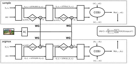
Figure 2.
Overview of the word gate (WG) model and the adaptive self-critical sequence training (ASCST) method. The adaptive SCST contains two components: the sample component and the argmax component. The sample component is regarded as the policy network of the reinforcement learning (RL) method. The inference component is the baseline method to make the training more stable. This harmonized learning with the inference can lower the variance of the gradients and improve the training procedure. FC is the full connected layer which projects the image vector to the word dictionary probabilities. CIDEr is an image captioning evaluation method proposed in [5].
3.2. Word Gate
In the neural image caption (NIC) model [9], the caption sentence is generated by an RNN, word-by-word. Given the target ground truth sequence , the RNN can be trained by minimizing the cross-entropy loss, as described in the NIC model [9]. The cross-entropy loss is formulated as:
where are the parameters of the RNN model, and I is an image vector. The probability is from the output of the RNN with a softmax function as follows:
where projects the hidden state to the prediction probability space and L is the size of the vocabulary.
Usually, L is pretty large and learning a distribution over such a large vocabulary space is a difficult task. However, when given a specific image, the candidate word set is usually small. For example, if the image is taken inside a room, then words like sofa, chair, wall, floor, etc. are in high probability to be the candidate words, while words such as train and river should not appear. Therefore, in order to reduce the prediction space, we introduce a gate mechanism for the words in the vocabulary, termed as the word gate (WG). In WG, the predicted distribution is gated by its gating score, which can be formulated as:
where is the word gate vector, to decide whether a word in the vocabulary should be a predicted candidate word, and ⊙ means the element-wise product. is the output of the LSTM at the last time. is the weight. The function is used to normalize the whole prediction of the LSTM.
The input of the LSTM is an embed vector. The embed vector is a continuous vector space with a much lower dimension which is converted from a space with one dimension per word or per image conception. Learning the gating score vector o is directly based on images without the need to consider syntax. As shown in Figure 3, a CNN is used to get the image feature I. Then, a fully connected layer is added to map the K-dimensional image vector to an L-dimensional embed vector, where K is the size which is same as that of the LSTM input and L is the size of the vocabulary. Then, we add a sigmoid layer to get the probability of all the words. We use the binary cross-entropy loss to train the WG:
where is the word probability learned from the image. is an indicator vector. If one word occurs in the caption, the corresponding position in t will be set to 1. The image feature used for the word gate is the same as the input of LSTM, and this could improve the learning performance of the image embedding vector.This image feature, which represents the global information of the image, is different from the spatial image matrix used in the attention, and its dimension is the same as that of the word embedding feature. The image embedding layer is equivalent to being trained twice and this layer can get better semantic information of the image.
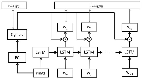
Figure 3.
The structure of the word gate model. The word gate model is trained by the binary cross-entropy loss. The LSTM model is trained by the cross-entropy loss. The output of the LSTM computes with the output of the word gate to get better dictionary probabilities.
Finally, we use the sum of the two losses as our final loss, which is given as:
where is the hyperparameter to decide the weight of these two losses. In this paper, we empirically set .
During testing, the WG first predicts a gating vector for all the words in the vocabulary. Then, the RNN generates the sentence word-by-word, predicting their distribution in each time step. The probability distribution is gated by the gating vector, and the final probabilities are output for each word.
The word gate is different from the image attributes used in [12]. Image attributes usually use the top 1000 words to train the CNN model. The image attribute model replaces the normal CNN to get the image vector which is the input to the LSTM. The word gate model does not need to train the attribute model independently. The CNN of the word gate is the same as the one used in [9], and it can be trained jointly. Furthermore, we do not need to select the top 1000 words—we use the whole vocabulary to learn the probabilities of all the words.
3.3. Adaptive Self-Critical Sequence Training
Similar to [1], we can cast image captioning as an RL problem, in which the “agent” (the LSTM) interacts with the external “environment” (i.e., words and image features). At each episode of the training process, the agent takes a sequence of “actions” (the predictions of the next word, ) according to a policy (the parameters of the network, ), and observes a “reward” R (e.g., the CIDEr score) at the end of the sequence. The goal of training is to find a policy (the parameters) of the agent that maximizes the following expected reward:
where is a sentence sampled from and is the words sampled at time step t. Using the REINFORCE algorithm [13], the gradient can be computed as:
In practice, the expectation can be approximated with a single Monte Carlo sample from the following distribution of actions:
However, the Monte Carlo estimation method is not stable, especially when the policy changes in the runtime, which usually causes high variance in the estimated gradient. A common solution is to reduce the following variance by shifting the reward with a “baseline” B:
where B can be any function that is independent with the action . The optimal baseline that yields the lowest variance estimator on is the following expected reward:
Finally, using the REINFORCE algorithm with a baseline B, the gradient of (the input to the softmax) is given as [1]:
For the full derivation of the gradients, please refer to [13,15] and Chapter 13 in [16].
Self-critical sequence training [4] gives a typical implementation of the RL-based method. Its core idea is to estimate the baseline with the reward obtained from the current policy model in testing reference:
where is the reward obtained by the Monte Carlo sampling, and is the reward obtained by the current model at the inference stage. If is higher than , the probability of these samples will be increased. If is lower than , this probability will be suppressed. Since the SCST baseline is based on the test-time estimate under the current model, it improves the performance of the model under the inference algorithm used at test time. This ensures the training/test time consistency and makes it possible to optimize with evaluation metrics directly. Self-critical sequence training minimizes the impact of baseline with the test-time inference algorithm on training time, which requires only one additional forward pass. It makes it so the model is optimized quickly, converges easily, and has a lower variance. Self-critical sequence training can be more effectively trained on mini-batches of samples with stochastic gradient descent (SGD).
The beam search method is a heuristic search algorithm that explores a graph by expanding the most promising node in a limited set. This method is widely used in the natural language generation model. SCST uses greedy decoding to select the current action for the baseline estimation in time step t:
This is used as the foundation of the beam search method, and the original training method with cross-entropy loss optimizes the probability of the max.
However, this method only considers the single-word probability, while the Monte Carlo sampling considers the probabilities of all words in the vocabulary. This inequivalence is harmful, since the aim of is to give a baseline for , but its value is computed in a very different way. Furthermore, we found that this greedy strategy causes SCST to be unstable in the training progress. As shown in Figure 4b, in SCST, the greedy reward () has higher variance than the Monte Carlo sampling reward (), and their gap is also very unstable. As a result, the CIDEr score in Figure 4a of SCST is lower than that of adaptive SCST.
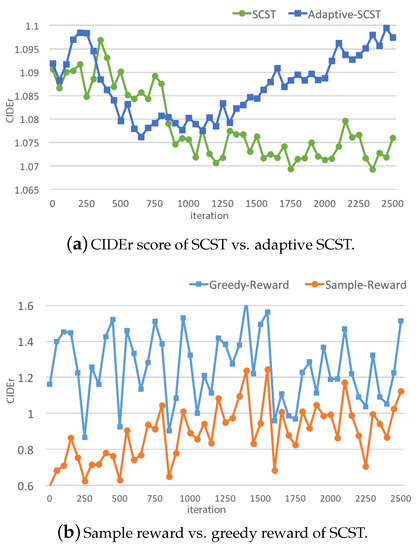
Figure 4.
The above two figures show the unstable training problem of SCST. The x-axis is the number of iterations, and the y-axis is the CIDEr score. Image (a) shows the plot of CIDEr score over iterations of SCST and our adaptive SCST, and image (b) shows the rewards (sample reward and greedy reward) of each iteration of SCST. All models were trained with the MSCOCO dataset [8].
In order to stabilize the estimation of baseline, we introduce a factor for as follows:
We argue that there exist at least two criteria for the factor : on one hand, it should be able to normalize so that will not shift severely; on the other hand, it must stabilize the gap between and to ensure that the gradient will not change rapidly. To this end, we formulate the factor in such a way that it not only takes account of the history of , but also considers the average level of . So, the factor is formulated as:
where denotes the expectation of the reward. In this formulation, is used to normalize the current greedy baseline with its expectation, and ensures the baseline has a similar level with the expectation value of . It is not realistic to compute and . Instead, we use the mean value of in previous v iterations (once the optimization for a mini-batch is defined as an iteration) as a estimation for the expectations.
Although the history factor can normalize the greedy baseline and stabilize the gap between and , it may lead the absolute value of the gap to an incorrect level (e.g., the loss may keep a negative value). Thus, we further introduce another factor to adjust the tradeoff of and . The final equation is shown as follows:
where is the in the ith iteration. Here we assume that t is the current iteration and h, which is called “history factor”, determines how many previous rewards are used to estimate the difference. Different from the history factor, is a hyper-parameter which was empirically set to be 0.9.
Our experiments show that the adaptive SCST method became more stable and reliable than the SCST method. It could reduce the variance of the gradient estimate, and we got better performance based on the adaptive SCST model.
4. Experiments
4.1. Dataset
We used the MSCOCO dataset [8], which is now the largest dataset of the image caption task to evaluate the performance of the proposed models. The official MSCOCO dataset includes 82,783 training images, 40,504 validation images, and 40,775 testing images. The image captioning model was evaluated on the offline testing dataset and the online server. For offline evaluation, we used the same dataset splits as in [17], which in recent papers have usually been used as offline evaluation. The training set in the offline dataset contains 113,287 images, and every image has five captions. We used a dataset of 5000 images for the validation and report results on a testing dataset of 5000 images.
We used words which appeared more than five times in all captions. In the end, we obtained a vocabulary with 9487 words. Words which occurred less than five times were replaced with the unknown token . We counted the length of all captions and found that the lengths of 97.7% captions were less than 16. We truncated the words to maintain the maximal length of the caption at 16.
4.2. Implementation Details
We used the feature map of the final convolution layer in the Resnext_101_64x4d [18] model to be regarded as our image feature. This model was pre-trained on the ImageNet dataset [19]. For the LSTM network, we set the hidden unit dimension to be 512 and the mini-batch to be 16. In order to avoid the gradient explosion problem, we used the gradient cutting strategy proposed in [20]. If the gradient was higher than 0.1, we set the gradient to be 0.1. In order to prevent the LSTM network from over-fitting, we added the dropout layer at the output of LSTM. We used the Adam method [21] to update the CNN and LSTM parameters. For the language model part, the initial learning rate was . For the convolution neural network, the initial learning rate was . The momentum and the weight decay were 0.8 and 0.999, respectively. We utilized the PyTorch deep learning framework to implement our algorithm. In testing, we used the beam search algorithm for better description generation. In practice, we used a beam size of 2.
In order to further verify the effect of the algorithm, we conducted a comparative experiment with the soft attention model. We selected our best model based on the CIDEr score as the initialization for the adaptive SCST training. We ran the adaptive SCST training by using Adam with a learning rate of .
We added the word gate method to the soft attention model, and the soft attention model was our baseline to evaluate the performance of our word gate method.
4.3. Results
We used CIDEr [5], BLEU [22], METEOR [23], and ROUGE_L metrics to evaluate the quality of the generated sentences.
In practice, we found that the reward obtained from the sample and the reward obtained from the greedy method were very different. This made the training loss become large, as shown in Figure 2. For comparison, we used both SCST and ASCST to fine-tune the same WG model. In Figure 2, the scores were evaluated every 50 iterations under the MSCOCO testing dataset. They were both trained with the same initial model, whose CIDEr was 1.092. From Figure 2, we can find that the ASCST model had better performance than the original SCST method. At the beginning of the RL, the SCST method obtained a lower result than the initial model, but ASCST was not affected by the difference of the two rewards, and it could improve the CIDEr score continuously.
In Table 1, we report the performance of the soft attention (Resnext_101_64x4d) baseline model [10], then we add the proposed word gate model (WG) to the baseline model without RL. Finally, we add SCST and ASCST to the soft attention + WG model for the comparison between the SCST method and the ASCST method. The above models were all validated on the test portion of the Karpathy splits, and they were all single models without ensemble method. From Table 1, we can find that the soft attention with WG model yielded a better performance than the soft attention model alone. Furthermore, to compare the SCST and the ASCST, we fine-tuned the same soft attention + WG model with the SCST method and ASCST method. Then, we obtained the soft attention + WG + SCST model and the soft attention + WG + ASCST model. From the results, we could find that the soft attention + WG + ASCST model had better performance than the soft attention + WG + SCST model reported in [4] on BLEU, ROUGE-L, and CIDEr metrics. This result shows that the proposed WG method could help the model to obtain better performance. Moreover, the ASCST could not only make the lRL training more stable, but could also improve the model’s performance. Compared with other state-of-the-art methods, our model also achieved competitive results.

Table 1.
Single-model image captioning performance without RL on the MSCOCO Karpathy test split. BLEU-n is a geometric average of precision over 1-to n-grams.NIC: neural image caption.
We then used our best model to get the test results with the official test split, and submitted our results to the official MSCOCO evaluation server. In Table 2, the state-of-the-art results on the leaderboard are also depicted. We outperformed the baseline method on all evaluation metrics.
Table 2.
Automatic evaluation on the online official MSCOCO [8] test split.
To further evaluate the ASCST method and get the appropriate hyper-parameters settings, we tried several comparison experiments where only h or in Equation (16) were different. In Figure 5 and Figure 6, we present the model with different h and settings. In Figure 5, we can find that the alpha_5000_beta_08 model had the best CIDEr score among these models ( alpha_5000 means the WG model trained with the ASCST method with h set to be 5000 iterations). From Figure 6, we can see that the performance of our model was significantly influenced by the . Figure 6 shows the influence of the hyper-parameter h. alpha_h_beta_08 refers to the WG model trained with the ASCST method with set to 0.8, and the h represent different hyper-parameters for the history factor. We found that with longer history reward information, better performance was obtained. In practice, set to be 0.8 and h set to be more than 2500 iterations could help our model to yield better performance.
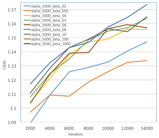
Figure 5.
The CIDEr scores of the WG-ASCST model with different . The x-axis is the number of iterations, and the y-axis is the CIDEr score. All the models in this figure have the same alpha. alpha_5000_beta_01 means the of the ASCST model is 0.1.
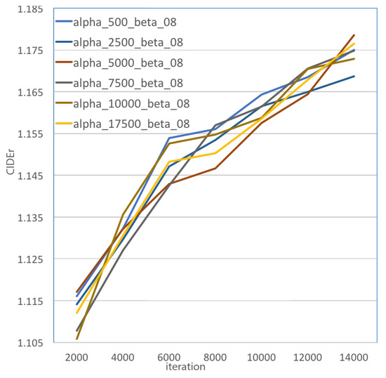
Figure 6.
The CIDEr scores of the WG-ASCST model with different h history rewards. The x-axis is the number of iterations, and the y-axis is the CIDEr score.
4.4. Quantitative Analysis
As shown in Figure 7, we selected some samples from the local test set for reference, and we can see that the model could generate readable text content and maintain rich semantic information about the image. For example, in the first image of Figure 7, we can see the generated text “a group of people playing tennis on a tennis court”. The generated caption successfully describes people and tennis in the image. In the second image of Figure 7, we can see our model could recognize people and skis in the image, and furthermore it could determine that people were standing in the snow.
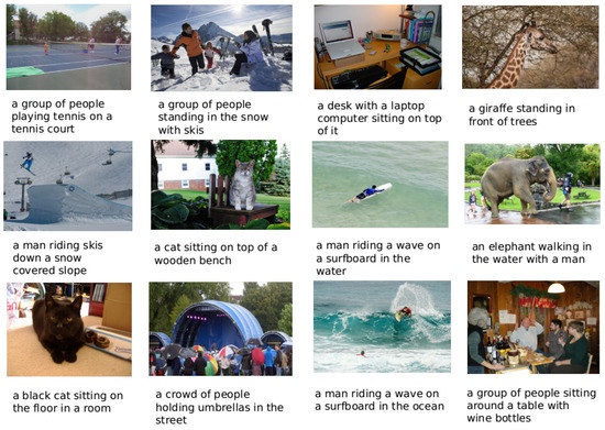
Figure 7.
Example of generated captions.
5. Conclusions
We present two innovations under the RL mechanism to boost the image captioning performance. First, a word gate function is introduced into the LSTM-based decoder model to reduce the search scope of the vocabulary for the sequence generation. Second, during the gradient updating along with the self-critic learning framework, two additional control parameters are defined to rescale the baseline with history reward information, in order to lower the variance of the expected reward. Finally, extensive experimental results show that the two innovations jointly obtained a boosted captioning performance and increased the stability of model training. Furthermore, we obtained impressive performance on the MSCOCO benchmark compared with some state-of-the-art approaches. We intend to study the application of the proposed method in the field of digital virtual asset security in future research.
Author Contributions
X.Z., L.L., J.L. and H.P. conceived and designed the experiments; X.Z. performed the experiments; X.Z., L.L., J.L. and H.P. analyzed the data; X.Z., L.L., L.G., Z.F. and J.L. wrote the paper. All authors interpreted the results and revised the paper.
Acknowledgments
This work is supported by the National Key Research and Development Program of China (Grant No. 2016YFB0800602) and the National Natural Science Foundation of China (Grant Nos. 61771071, 61573067).
Conflicts of Interest
The authors declare no conflict of interest.
References
- Ranzato, M.; Chopra, S.; Auli, M.; Zaremba, W. Sequence level training with recurrent neural networks. arXiv 2015, arXiv:1511.06732. [Google Scholar]
- Bengio, S.; Vinyals, O.; Jaitly, N.; Shazeer, N. Scheduled sampling for sequence prediction with recurrent Neural networks. arXiv 2015, arXiv:1506.03099. [Google Scholar]
- Liu, S.; Zhu, Z.; Ye, N.; Guadarrama, S.; Murphy, K. Improved Image Captioning via Policy Gradient optimization of SPIDEr. In Proceedings of the 2017 IEEE International Conference on Computer Vision (ICCV), Venice, Italy, 22–29 October 2017. [Google Scholar]
- Rennie, S.J.; Marcheret, E.; Mroueh, Y.; Ross, J.; Goel, V. Self-critical Sequence Training for Image Captioning. arXiv 2016, arXiv:1612.00563. [Google Scholar]
- Vedantam, R.; Zitnick, C.L.; Parikh, D. CIDEr: Consensus-based image description evaluation. arXiv 2015, arXiv:1411.5726. [Google Scholar]
- Mnih, A.; Gregor, K. Neural Variational Inference and Learning in Belief Networks. arXiv 2014, arXiv:1402.0030. [Google Scholar]
- Bahdanau, D.; Brakel, P.; Xu, K.; Goyal, A.; Lowe, R.; Pineau, J.; Courville, A.; Bengio, Y. An actor-critic algorithm for sequence prediction. arXiv 2016, arXiv:1607.07086. [Google Scholar]
- Lin, T.; Maire, M.; Belongie, S.J.; Hays, J.; Perona, P.; Ramanan, D.; Dollar, P.; Zitnick, C.L. Microsoft COCO: Common Objects in Context. arXiv 2014, arXiv:1405.0312. [Google Scholar]
- Vinyals, O.; Toshev, A.; Bengio, S.; Erhan, D. Show and tell: Lessons learned from the 2015 mscoco image captioning challenge. IEEE Trans. Pattern Anal. Mach. Intell. 2017, 39, 652–663. [Google Scholar] [CrossRef] [PubMed]
- Xu, K.; Ba, J.L.; Kiros, R.; Cho, K.; Courville, A.C.; Salakhudinov, R.; Zemel, R.; Bengio, Y. Show, Attend and Tell: Neural Image Caption Generation with Visual Attention. arXiv 2015, arXiv:1502.03044. [Google Scholar]
- Wu, Q.; Shen, C.; Liu, L.; Dick, A.R.; Den Hengel, A.V. What Value Do Explicit High Level Concepts Have in Vision to Language Problems. arXiv 2016, arXiv:1506.01144. [Google Scholar]
- Yao, T.; Pan, Y.; Li, Y.; Qiu, Z.; Mei, T. Boosting Image Captioning with Attributes. arXiv 2016, arXiv:1611.01646. [Google Scholar]
- Williams, R.J. Simple statistical gradient-following algorithms for connectionist reinforcement learning. Mach. Learn. 1992, 8, 229–256. [Google Scholar] [CrossRef]
- Zhang, L.; Sung, F.; Liu, F.; Xiang, T.; Gong, S.; Yang, Y.; Hospedales, T.M. Actor-Critic Sequence Training for Image Captioning. arXiv 2017, arXiv:1706.09601. [Google Scholar]
- Zaremba, W.; Sutskever, I. Reinforcement Learning Neural Turing Machines-Revised. arXiv 2015, arXiv:1505.00521. [Google Scholar]
- Sutton, R.S.; Barto, A.G. Reinforcement Learning: An Introduction; MIT Press: Cambridge, MA, USA, 1998; Volume 1. [Google Scholar]
- Karpathy, A.; Feifei, L. Deep visual-semantic alignments for generating image descriptions. In Proceedings of the IEEE Conference on Computer Vision and Pattern Recognition, Boston, MA, USA, 7–12 June 2015; pp. 3128–3137. [Google Scholar]
- Xie, S.; Girshick, R.B.; Dollar, P.; Tu, Z.; He, K. Aggregated Residual Transformations for Deep Neural Networks. arXiv 2016, arXiv:1611.05431. [Google Scholar]
- Krizhevsky, A.; Sutskever, I.; Hinton, G.E. ImageNet Classification with Deep Convolutional Neural Networks. In Proceedings of the 25th International Conference on Neural Information Processing Systems, Lake Tahoe, NV, USA, 3–6 December 2012; pp. 1097–1105. [Google Scholar]
- Sutskever, I.; Vinyals, O.; Le, Q.V. Sequence to Sequence Learning with Neural Networks. arXiv 2014, arXiv:1409.3215. [Google Scholar]
- Kingma, D.; Ba, J. Adam: A method for stochastic optimization. arXiv 2014, arXiv:1412.6980. [Google Scholar]
- Papineni, K.; Roukos, S.; Ward, T.; Zhu, W.J. BLEU: A method for automatic evaluation of machine translation. In Proceedings of the 40th Annual Meeting on Association for Computational Linguistics, Philadelphia, PA, USA, 7–12 July 2002; pp. 311–318. [Google Scholar]
- Denkowski, M.; Lavie, A. Meteor Universal: Language Specific Translation Evaluation for Any Target Language. In Proceedings of the Ninth Workshop on Statistical Machine Translation, Baltimore, MA, USA, 26–27 June 2014; pp. 376–380. [Google Scholar]
- Jia, X.; Gavves, E.; Fernando, B.; Tuytelaars, T. Guiding the Long-Short Term Memory Model for Image Caption Generation. arXiv 2015, arXiv:1509.04942. [Google Scholar]
- Zhou, L.; Xu, C.; Koch, P.; Corso, J.J. Image caption generation with text-conditional semantic attention. arXiv 2016, arXiv:1606.04621. [Google Scholar]
- Yang, Z.; Yuan, Y.; Wu, Y.; Salakhutdinov, R.; Cohen, W.W. Review Networks for Caption Generation. arXiv 2016, arXiv:1605.07912. [Google Scholar]
- You, Q.; Jin, H.; Wang, Z.; Fang, C.; Luo, J. Image Captioning with Semantic Attention. arXiv 2016, arXiv:1603.03925. [Google Scholar]
© 2018 by the authors. Licensee MDPI, Basel, Switzerland. This article is an open access article distributed under the terms and conditions of the Creative Commons Attribution (CC BY) license (http://creativecommons.org/licenses/by/4.0/).