Speckle Reduction on Ultrasound Liver Images Based on a Sparse Representation over a Learned Dictionary


School of Electrical Engineering and Computer Science, Gwangju Institute of Science and Technology, Gwangju 61005, Korea
*
Author to whom correspondence should be addressed.
Appl. Sci. 2018, 8(6), 903; https://doi.org/10.3390/app8060903
Submission received: 20 April 2018
/
Revised: 28 May 2018
/
Accepted: 28 May 2018
/
Published: 31 May 2018
(This article belongs to the Special Issue Ultrasound B-mode Imaging: Beamforming and Image Formation Techniques)
Abstract
:Ultrasound images are corrupted with multiplicative noise known as speckle, which reduces the effectiveness of image processing and hampers interpretation. This paper proposes a multiplicative speckle suppression technique for ultrasound liver images, based on a new signal reconstruction model known as sparse representation (SR) over dictionary learning. In the proposed technique, the non-uniform multiplicative signal is first converted into additive noise using an enhanced homomorphic filter. This is followed by pixel-based total variation (TV) regularization and patch-based SR over a dictionary trained using K-singular value decomposition (KSVD). Finally, the split Bregman algorithm is used to solve the optimization problem and estimate the de-speckled image. The simulations performed on both synthetic and clinical ultrasound images for speckle reduction, the proposed technique achieved peak signal-to-noise ratios of 35.537 dB for the dictionary trained on noisy image patches and 35.033 dB for the dictionary trained using a set of reference ultrasound image patches. Further, the evaluation results show that the proposed method performs better than other state-of-the-art denoising algorithms in terms of both peak signal-to-noise ratio and subjective visual quality assessment.
1. Introduction
In the last 20 years, there has been growing interest in the use of ultrasound imaging for a variety of applications, such as observing the blood flow through an organ or other structures; determining bone density; imaging the heart, a fetus, or ocular structures; or diagnosing cancers [1,2]. Ultrasound imaging has been widely applied owing to its ability to produce real-time images and videos. Ultrasound images are captured in real-time by transmitting high frequency sound waves through body tissue. It comprises an array of transducer elements that sequentially echo the signal for each spatial direction to generate a raw line signal. The scan is converted to construct a Cartesian image from the processed raw line signal [2].
In recent years, many researchers have attempted to develop computer-aided diagnostic (CAD) systems for diagnosing liver and breast cancers [3,4,5,6] based on ultrasound imaging. The aim of these systems is to differentiate benign and malignant lesion tissues as well as cysts [7]. A CAD system carries out the diagnosis in four stages: data preprocessing, image segmentation, feature extraction, and classification [4]. Data preprocessing is the first and most vital step in the CAD system process because it reconstructs an image without eliminating the important features by reducing signal-dependent multiplicative noise called speckle [8].
The development of a precise speckle reduction model is an important step to achieve efficient denoising filter design. Recent review articles [4,9], reported that speckle reduction filters are categorized into two broad approaches: spatial filtering and multiscale methods. Techniques under spatial domain filtering include enhanced Frost filtering [10], Lee filtering [11], mean filtering [12], Wiener filtering [13], Kuan filtering [14], and median filtering [15]. Spatial filters utilize local statistical properties to reduce speckle noise. However, small details may not be preserved [9]. Several methods [16,17,18,19] use multiscale filtering, which uses the wavelet transform to preserve the image signal regardless of its frequency content. Donoho et al. [20] proposed reducing noise in the wavelet domain by soft thresholding. However, their approach lacked translation invariance when using the discrete wavelet transform. This is resolved by eliminating up and down samplers in the wavelet transform by using a stationary wavelet transform [21], which is a redundant technique because the number of input and output samples at each level is the same. A multiresolution technique called translation invariant image enhancement was proposed in [22]. The proposed technique incorporates noise reduction and directional filtering. Directional filtering is executed using eigenvalues by analyzing the structure of each pixel’s neighborhood. Rudin et al. [23,24] and Perona et al. [25] proposed successful image denoising techniques called total variation (TV) and anisotropic smoothing, respectively. These models were improved and extended upon in later works [26,27]. However, all these methods are computationally expensive. In recent years, more efficient denoising techniques such as sparse representation (SR) have been proposed [28,29,30,31]. In digital image processing, many signals are sparse; i.e., they contain many coefficients either equal to or close to zero in a specific domain. The objective of SR is to efficiently reconstruct the signal with a linear combination of a few dictionary atoms from the transformed signal domain [32].
This study was conducted with the objective of developing filtering algorithm that can reduce noise without losing significant features or eliminating edges. To this end, this paper proposes, a technique that reduces the speckle noise in ultrasound imaging systems by applying a relatively new signal reconstruction model known as SR [32] to deal with complicated noise properties. Sparse representation provides superior estimation even in an ill-conditioned system [33], and has been found to be very useful in medical imaging applications. However, one challenge of designing this system is the presence of a multiplicative speckle signal because dictionary learning methods are not effective on multiplicative and correlated noise. We overcome this by using two different methods. Firstly, the speckle noise is transformed into additive noise using an enhanced homomorphic filter that can also capture high and low frequency signal of the image. Secondly, we introduced TV regularization of the image and sparse prior over learned dictionaries. Total variation regularization is efficient for noisy image, while the patch-based dictionaries are well adapted to texture features [34], and reduces the artifacts in smooth pixel regions [35]. The advantage of the sparse prior is that it utilizes fewer dictionary columns to reconstruct a noiseless ultrasound image without losing many important features of the signal. Therefore, in our proposed model we combined the two approaches, the patch-based SR over learned dictionaries and the pixel-based TV regularization method, for efficient speckle reduction. The K-singular value decomposition (KSVD) algorithm [36] is used to learn two modified dictionaries from reference ultrasound image datasets and the corrupted images; these are referred to as dictionaries 1 and 2, respectively. The results are evaluated on both dictionaries and compared with conventional algorithms to show that the speckle noise is suppressed effectively in the ultrasound image using SR.
The rest of the paper is organized as follows. Noise model and related works are described in Section 2. The proposed SR framework for speckle reduction in ultrasound imaging is presented in Section 3. In Section 4, the experiments and results obtained are discussed. The paper is concluded in Section 5.
2. Background
2.1. Ultrasound Noise Model
Ultrasound imaging system are often affected by multiplicative speckle [37]. Scattering time differences lead to constructive and destructive interference of the ultrasound pulses that are reflected from biological tissues. Speckle patterns can be classified depending on the spatial distribution, number of scatters per resolution cell, and properties of the imaging system [9]. Speckle noise affects the detectability of the target and reduces the contrast and resolution of the images, making it difficult for a clinician to provide a diagnosis.
In ultrasound, the multiplicative noise models are based on the product of the original signal and noise. Thus, the intensity of a noisy signal depends on the original image intensity. The mathematical expression for a multiplicative speckle model is given by
where is the speckled image, is the original image, and is the speckle noise. The spatial location of an image is represented using indexes i and j, where index i ranges from 1 to N, and index j from 1 to M.
2.2. Related Work on Multiplicative Noise Reduction
Several algorithms have been proposed to deal with more complex multiplicative and additive speckle noise models [38]. For instance, the Kuan, Frost, Lee filters, and speckle reducing anisotropic diffusion (SRAD) filter [39] are effective on the multiplicative noise model. Other filters, specifically the median, Wiener, and wavelet filters [40], are designed for the additive noise model [4]. However, each filter has certain advantages and limitations [38]. In a few filter models, the quality of the processed image is affected by the window size: large window sizes cause image blurring, degrading the fine details of an image. Conversely, small window sizes do not denoise the image sufficiently. Other widely used multiplicative noise reduction algorithms are based on the TV regularization term [23,41], nonlocal methods [42,43], and wavelet-based approaches [16]. Total variation-based methods effectively remove flat-region-based noise and preserve the edges of images. However, fine details are lost because of over-smoothed textures. Nonlocal algorithms depend on similarities of image patches. Their performance is limited by dissimilar image patches. However, wavelet-based approaches preserve texture information better than TV-based methods. This approach assumes that images in the SRs are based on a fixed dictionary [29,36]. However, certain characteristics of the processed image might not be captured because the dictionary does not contain any similar image content.
To overcome the above disadvantages, over the past few years, researchers have sought to develop an algorithm based on SR in the field of image and signal processing [32]. This is because the pattern similarities of image signals such as textures and flat regions, mean that the signal can be efficiently approximated as a linear combination using a dictionary of only a few functions called atoms [29,34,36]. Elad and Aharon [36] proposed an image denoising algorithm using an adaptive dictionary called KSVD that is based on sparse and redundant representations. It includes sparse coding and dictionary atoms that are updated to better fit the data. The advantage of KSVD compared to fixed dictionaries is that it is effective at removing additive Gaussian noise using the linear combinations of a few atoms, by learning a dictionary from noisy image patches and then reconstructing each patch.
A dictionary , composed of Nc columns of Nr elements, is called a sparse-land model [36]. K-singular value decomposition seeks the best signal representation of image signal y from the sparsest representation :
where the vectorization of is denoted by vector and is the few number of non-zero entries in . K-singular value decomposition replaces the dictionary update and sparse coding stages with a simple singular value decomposition. The orthogonal matching pursuit (OMP) method [44] is an effective method to find the sparse approximation. In the OMP, if the noise level is below the approximation, the image patches are rejected. The singular value decomposition constructs better atoms by combining patches to reduce noise for ultrasound speckle reduction. K-singular value decomposition has also proved to effectively reduce the speckle produced by additive white Gaussian noise on corrupted images [29,36].
The filtering algorithm comprises two steps. First, the dictionary is trained from a set of image data patches or from noisy image patches based on KSVD. The next step uses to compute SR using dictionary A and denoises the image [29].
The method proposed in [45] also uses a dictionary learning approach for denoising ultrasound images. A homomorphic filter is used to convert multiplicative noise into additive white Gaussian noise and then the noiseless signal is reconstructed over image patches (atoms) to create the SR from a learned dictionary. However, noise in flat regions still exists and poor edges make the reconstructed images difficult to analyze. In [34], the authors proposed an image denoising technique that operates directly on multiplicative noise and is based on three terms: SR over an adaptive dictionary, a TV regularization term, and a data-fidelity term. However, the proposed model is nonconvex because of the product between the unknown dictionary and sparse coefficients and the data-fidelity term is a log function. Therefore, solving the squared norm is difficult. This optimization problem is overcome by the split Bregman technique. However, these methods do not contain high- and low-frequency components of the image. We obtain this information using an enhanced homomorphic filter designed to improve the final image. Furthermore, we utilize the advantages of combining a TV regularization term and SR learned over two modified dictionaries.
3. Sparse Representation Framework for Speckle Reduction
As discussed above, we define our proposed scheme for ultrasound speckle reduction by considering the multiplicative noise model [37] obtained by an ultrasound transducer. Equation (1) can thus rewritten as
where is the degraded B-mode image signal [46], represents the ideal image that must be recovered, and represents the speckle noise, generally modelled as a Rayleigh probability density function with random variables [11,47]. Each term includes coordinates defined according to the acquisition geometry.
In general, a homomorphic filter [48] is a well-proven technique for converting multiplicative noise. In this study, we modified it by taking the log of the multiplicative noisy signal and filtering the image using a Butterworth high-pass (BW-HP) filter to attenuate low frequencies in the transmitted signal while preserving the high frequencies in the reflected component. The equation of the BW-HP filter is
where, D0 is the cut-off frequency and f is the order of the filter. We varied the frequency values u and v of the i and j spatial coordinates. We used the BW-HP filter because it generates fewer ringing artifacts on the image signal.
We also used a Gaussian low pass (GLP) filter to smooth the low-frequency signal component in the log domain. The equation of the GLP filter is
where D(u,v) is the distance from the origin in the frequency plane. Finally, the additive noise signals were estimated by applying inverse transform.
Figure 1 shows the steps used to convert an original noisy image into an image with additive noise using the enhanced homomorphic transform. This technique consists of five steps. We first take the log on both sides of Equation (2) and use a two-dimensional fast Fourier transform (FFT) to represent the image in the frequency domain. Then, the Fourier image is filtered with two filter functions, those are the BW-HP and GLP filters [12]. The BW-HP filter increases the contrast of the image signal corresponding to the high-frequency component. The GLP filter smooths the noise signal without eliminating the entire low-frequency component. Both filtered signals are applied to the two-dimensional inverse fast Fourier transform (IFFT). Finally, taking the exponent of the image, we obtain the transformed image. This process is discussed in detail below.
Step 1: Take the log on both sides of the and the signal; now the multiplicative noise can written as
After being transformed logarithmically, the signal now contains Gaussian additive noise [49]. We remove from the speckled ultrasound image by applying an additive noise suppression algorithm. Thus, the problem is now to estimate from noisy data.
Step 2: Apply FFT to convert the image into the frequency domain. Equation (5), thus becomes,
where, and are the FFT of and , respectively.
Step 3: Apply BW-HP and GLP to the by means of two filter function and from Equations (3) and (4) respectively in the frequency domain. The filtered version of is written as
Step 4: Take the inverse Fourier transform of Equation (7) to get the converted signal in the spatial domain
Step 5: Finally, we obtain the transformed image by taking the exponent of the image using the following equation
In this paper, we model the transformed image as additive noise degradation of the original image , i.e.,
This completes how we have used the homomorphic filter to transform the speckle noise into additive noise. The two filter functions are utilized to improve edge information by enhancing contrast and smooths the additive noise of the transformed image.
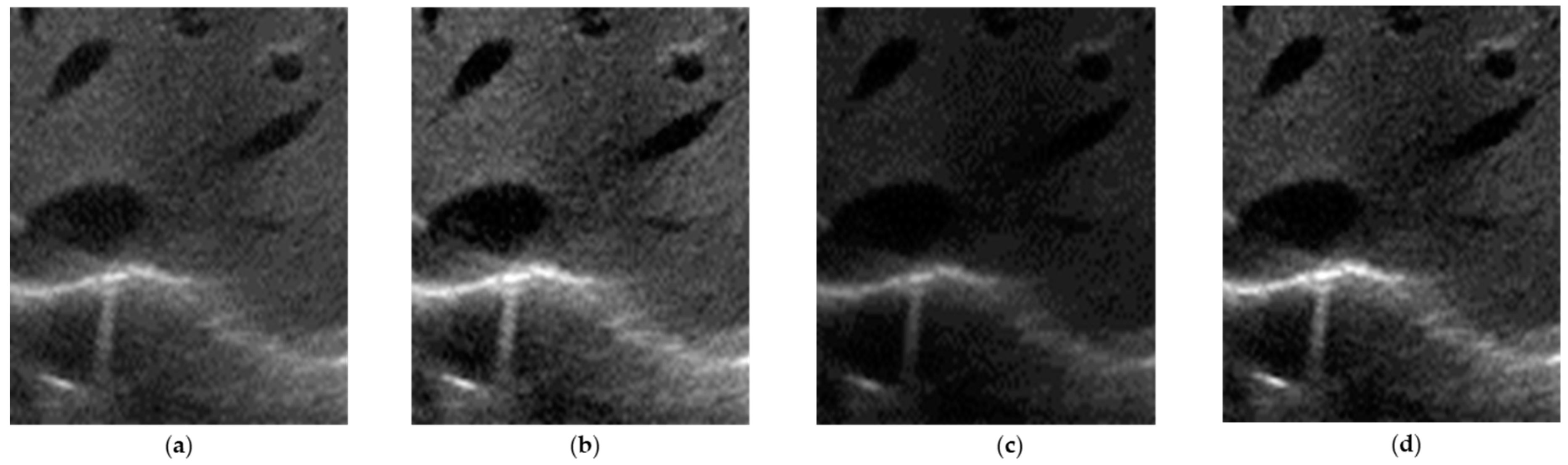
Figure 2 shows the output of the enhanced homomorphic filter at the BW-HP and GLP filter stages. It is clear that the image in Figure 2b has an increased intensity because the low frequency signal is attenuated and the image in Figure 2c is smoothed by the GLP filter. The sum of these two signals is the final transformed noisy image.
An ultrasound image can be represented as sparse in the gradient domain. We thus define here a difference signal. A pixel-based TV regularization can be performed on the transformed image for more effective denoising. The horizontal and vertical difference matrices are defined below [50].
Further, the difference signal of is defined as
We can show that there exists a dictionary with which the original image can be sparsely represented as
where is the vectorization of the recovered signal such that . If a signal is K-sparse in the dictionary for , we imply that the signal can be represented with K columns of the dictionary. The column vector is the vector of the coefficients. Then, by optimizing the following convex problem, the signal can be recovered:
In Equation (9), a column vector is the vectorization of the transformed image , note that . Also note that is a utility parameter selectable according to the noise strength. This convex constrained problem can be transformed into an unconstrained optimization problem using the Lagrange multiplier method [51]:
Using the unconstrained problem, we are able to combine a regularization term, which is weighted by parameter and a quadratic data-fidelity term. Equation (10) is not ready for use yet since we do not know the sparsity dictionary . Therefore, we use the following approach where the dictionary, the sparse representation coefficient vector , and the image vector are estimated altogether. The overall optimized discrete sparse model proposed in this paper, for denoising the ultrasound image, can be written as
where is an operation that extracts a square image patch from the transformed image located at the pixels of the image. The notation is used to imply the norm, which is the sum of the absolute values of the argument signal, which in this case is the difference signal . There are two positive parameters and used to balance the contribution of different terms. In Equation (11), the first and second terms are the TV regularization norm and the sparse representation prior. Optimization in Equation (11) seeks to find a solution with which each patch of the recovered image can be represented by a dictionary matrix with sparse coefficient in the sense of a bounded error. The norm gives the sparsity constraint which controls the sparsity coefficients of any small image patch.
As mentioned in Related Work Section 2.2, there is a sparse coding stage that utilizes the KSVD iterative process. In the first stage, sparse coding is performed assuming fixed and . In the second stage, dictionary is updated to minimize using known sparse coefficients and . The sparse coefficients are computed using the OMP method [52] because of its efficiency and simplicity. Elad et al. [29] showed that learning a dictionary trained from good quality image patches and noisy images results in better performance.
In this paper, we use two approaches to train the dictionary. The first approach is to use a group of image patches taken from many ultrasound reference images. We call the dictionary obtained from this approach Dictionary 1. The second approach is to use the corrupted images and call them Dictionary 2. We aim to compare the performance difference based on these two approaches. The comparison is made in the Results section.
It should be noted that Equation (11) is non-convex because of the non-differentiable TV regularization term and the product of the unknowns and . We overcome this by using the split Bregman iterative approach [53].
Overall, the proposed algorithm can be summarized as follows:
- Convert the multiplicative noise into additive noise using an enhanced homomorphic filter and capture the high- and low-frequency components to retain detailed information.
- Apply pixel-based TV regularization to smooth the filtered image signal.
- Apply patch-based sparse representation over a dictionary trained using the KSVD algorithm. We employed two modified dictionaries—one trained with a set of reference ultrasound image patches and another trained using the speckled image patches.
- Iterate between the TV regularization and sparse representation procedure to improve the reconstructed image.
Figure 3 summarizes the proposed algorithm.
3.1. Performance Estimation
The reconstructed denoised image using the proposed algorithm were compared with the original image. Two image quality metrics were used for quantitative performance measurements: peak signal-to-noise ratio (PSNR) and mean structural similarity (MSSIM) [54]. Peak signal-to-noise ratio is defined as:
where Nmax represents the maximum fluctuations in the input image. Here, Nmax = (2n − 1), Nmax = 255, when the components of a pixel are encoded using eight bits. N denotes the number of pixels processed, is the original signal, and is the recovered image signal. In MSSIM, the structures of the two images are compared after normalizing the variance and subtracting the luminance as follows:
where denotes luminance, denotes contrast, and denotes structure comparison functions. Further, and r are weighted parameters that are used to adjust the relative importance of the three components.
4. Experimental Results and Discussion
4.1. Simulations on Synthetic Images
In this section, we analyze the performance of the proposed approach on the synthetic Shepp–Logan phantom test image [55] (Figure 4a) with a speckle noise variance of σ = 10 (Figure 4b) of a 256 × 256 pixel size. This result helps us to understand the effectiveness of the simulated image, clearly determine the distinctive features of the image, and optimize the algorithm before testing on the clinical datasets. We compared the proposed algorithm with some standard speckle reduction filters for ultrasound liver images [4]. The compared algorithms were local statistical filters such as the Frost filter [10], Lee filter [11], 3 × 3 Weiner filter [13], Kuan filter [14], 3 × 3 median filter [15], and speckle reducing anisotropic diffusion (SRAD) filter [39]. In addition, multiscale filters such as wavelets [40] were evaluated. The despeckled images in Figure 4e–g show that the Frost, wavelet, and Kuan filters do not effectively reduce noise. In contrast, Figure 4h–j show that the median, Weiner, and SRAD filters, reduce most noise; however, the edges are not preserved and artificial noises can be introduced to a certain extent. This result verifies that the proposed SR technique reduces noise and preserves the edges better than the conventional methods on synthetic images. Table 1 shows the PSNR value and MSSIM value. The proposed algorithm reconstructs the original image with a PSNR value of 36.86 dB with Dictionary 1 and 37.04 dB with Dictionary 2.
4.2. Clinical Liver Ultrasound Images
The proposed algorithm efficiency was estimated using a set of B-mode greyscale ultrasound liver images. The images were obtained using the ECUBE 12R ultrasound research system from Alpinion medical systems, Seoul, Korea. The components used to generate the ultrasound images include a 128-element linear transducer at a center frequency of 5 MHz, a lateral beam width of 1.5 mm, and a pulse length of 1 mm. In our experiment, sparse coding was performed using two dictionaries with a 64 × 256 size, designed to handle patches of 8 × 8 size pixels (N = 64 and K = 256)—one trained from a noisy image and the other trained from a set of reference images.
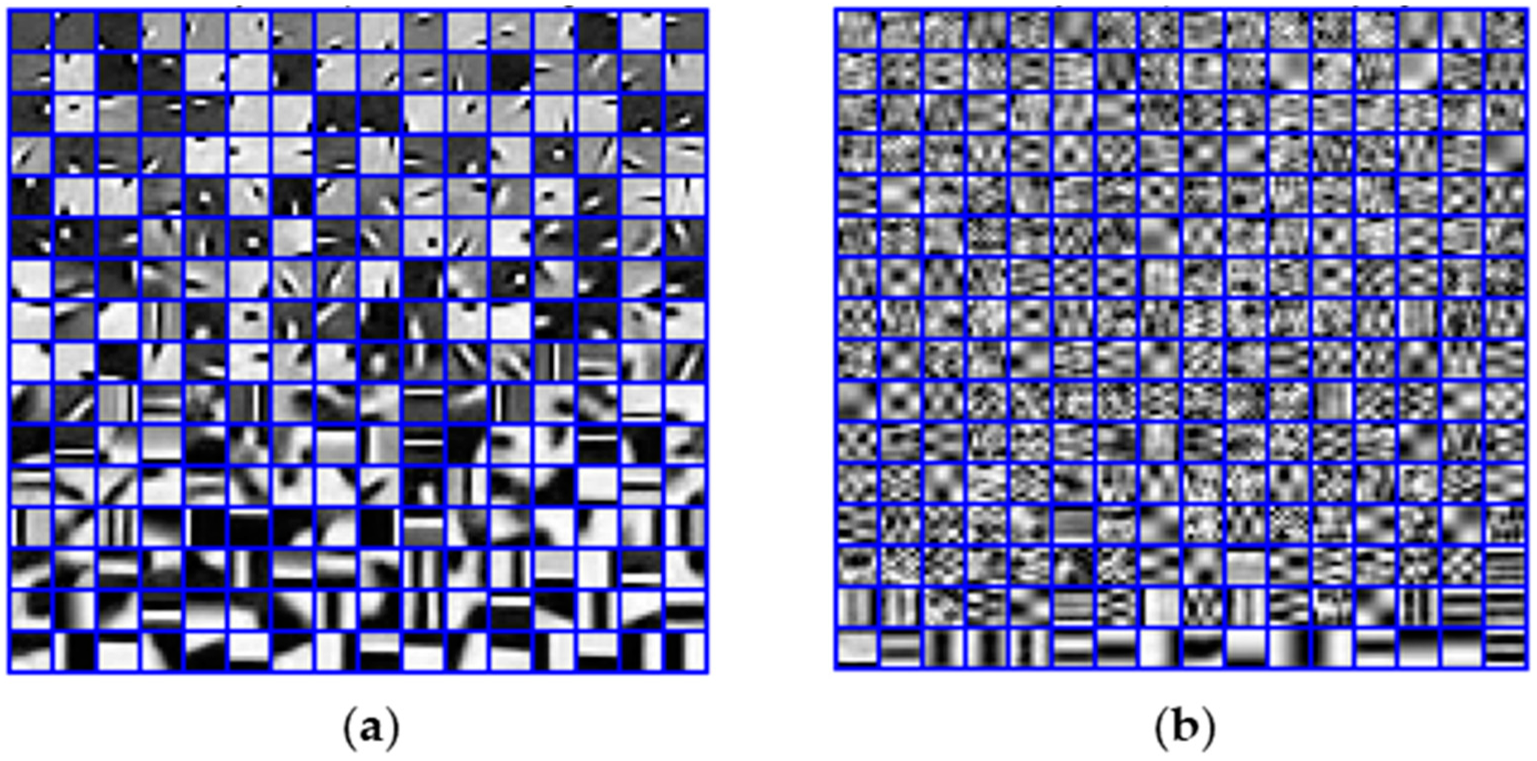
The training data were constructed from a dataset comprising 3245 reference ultrasound images. The random collection of 16 × 16 dictionary atoms (K = 256) is presented in Figure 5a and the dictionary trained on the noisy image itself by overlapping patches is represented in Figure 5b. Where, every dictionary atom occupies a cell of 8 × 8 pixel (N = 64). We performed the tests on the three ultrasound reference images shown in Figures 6a, 7a and 9a. The KSVD algorithm was initialized with a trained dictionary and executed 180 iterations, as recommended in [29].
The numerical evaluation was performed using PSNR and MSSIM (as discussed in Section 3.1) on the proposed algorithm and compared with the denoising methods Frost filter [10], Lee filter [11], 3 × 3 Weiner filter [13], Kuan filter [14], 3 × 3 median filter [15], SRAD filter [39], and wavelet filter [40].
Figure 6a, shows a right lobe liver image with size 256 × 256 pixels, where the lateral size is given by the x-axis, and the axial size is given by the y-axis. In this original image, we included a speckle noise parameter = 10 and the PSNR was calculated using Equation (12). It is clear that detailed information of the image is highly distorted, as shown in Figure 6b with a PSNR value of 28.148 dB. Figure 6c,d show the denoising results obtained by the proposed method using Dictionary 1 with a PSNR value of 35.033 dB and Dictionary 2 with a PSNR value of 35.537 dB. It is clear that the SR over learned dictionaries improves both edges and smooth features by eliminating the noise and reconstructs the image as much closer to the original image, as shown in Figure 6a.
Figure 7 shows the comparative experimental results obtained on real-time ultrasound images. For this experiment, we obtained a 256 × 256-pixel liver image of a healthy person with a PSNR value of 24.6271 dB. The radio frequency (RF) frames were obtained using a linear transducer with a frequency range of 8 MHz. This frequency range was selected because of its suitability for liver imaging, and we considered natural speckle noise for these experiments. The original speckled image was then denoised using the proposed algorithm with both dictionaries and also using conventional algorithms. To assess the speckle reduction, we selected two regions in of the speckled image. The two regions in the case of Figure 7a are displayed as a red square and a green square. The red one indicates the diaphragm of a liver and the green square shows the presence of an excessive noisy region observed from deeper tissue. The differences can be noticed from the filtered images in dashed red and the green square. Figure 7d–f show that detailed information lost by the blurring effect on the results obtained with Frost filter, median filter, and Kuan filter. In particular, the wavelet filter, Weiner filter, and the SRAD filter are not very effective in reducing speckle and perform poorly in retrieving sharp edge information, as can be seen in Figure 7g–i. Figure 7b shows the results for the proposed method using Dictionary 1 (PSNR = 30.3345 dB) and Figure 7c shows the results for the proposed method using Dictionary 2 (PSNR = 30.8073). It is clear that the image denoised using the proposed SR method reconstructed image very close to the original image. It can also be seen that the dictionary trained on the noisy image gives better results than using a set of multiple references images. The results of this comparative experiment show that the proposed algorithm not only reduces the speckle noise but also preserves the edge information. Table 2 shows the PSNR and MSSIM values to quantify the results numerically for noise parameter = 15.
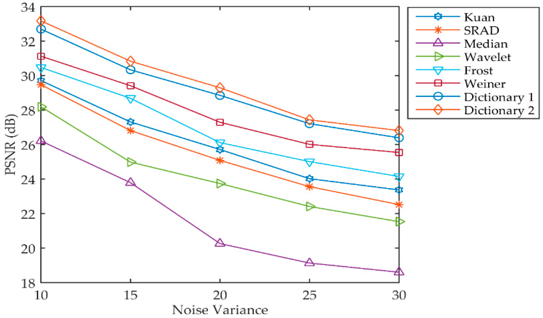
Speckle is an arbitrary granular texture noise that degrades ultrasound image quality. This experiment was performed to evaluate different noise variances by comparing the PSNR obtained using the proposed algorithm and other despeckling algorithms. The simulated result using the noise levels 10, 15, 20, 25, and 30 are illustrated in Figure 8. The results clearly depict that, for different noise variances, the proposed algorithm gives the best PSNR value of all the algorithms on speckle reduction.
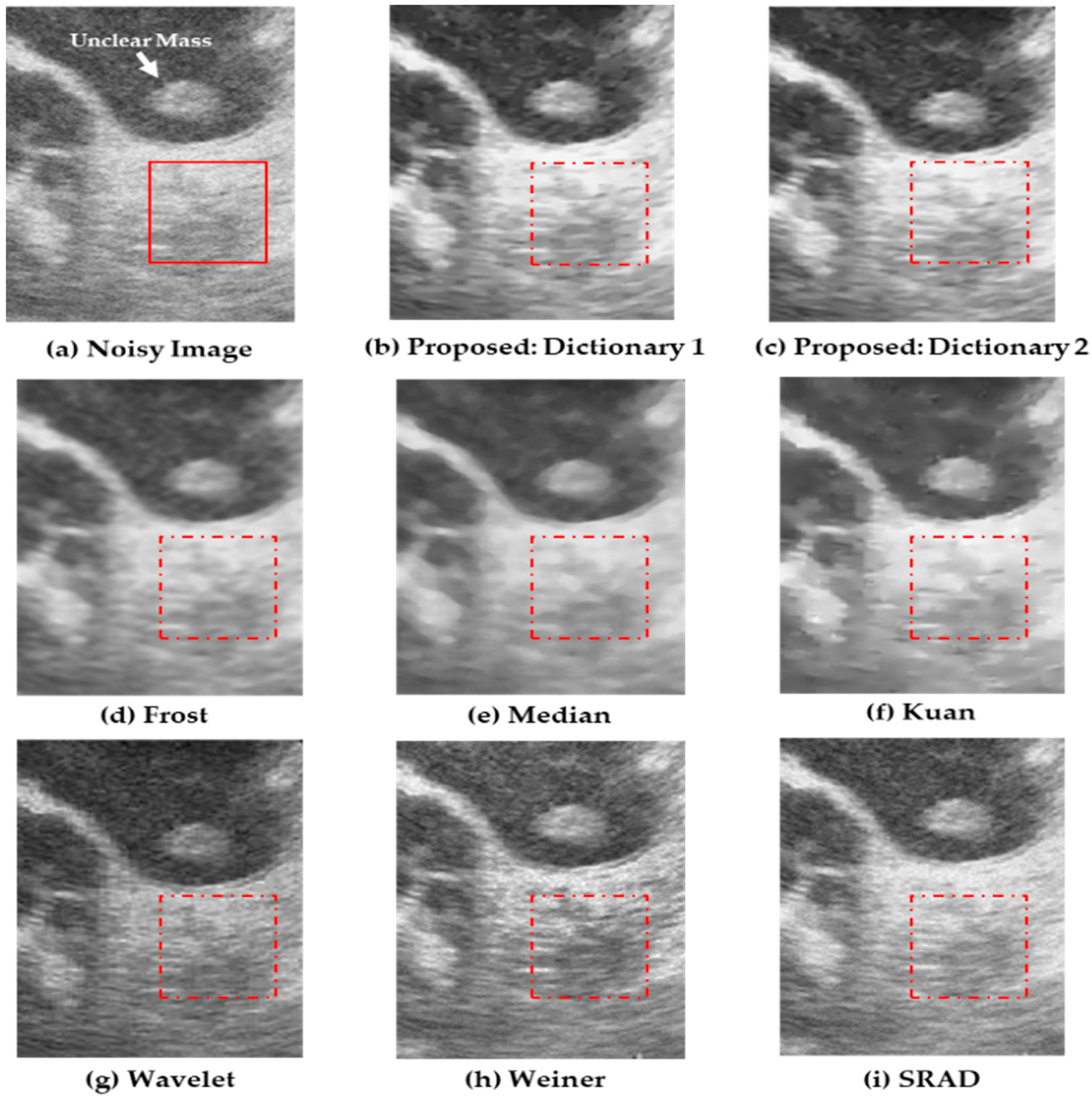
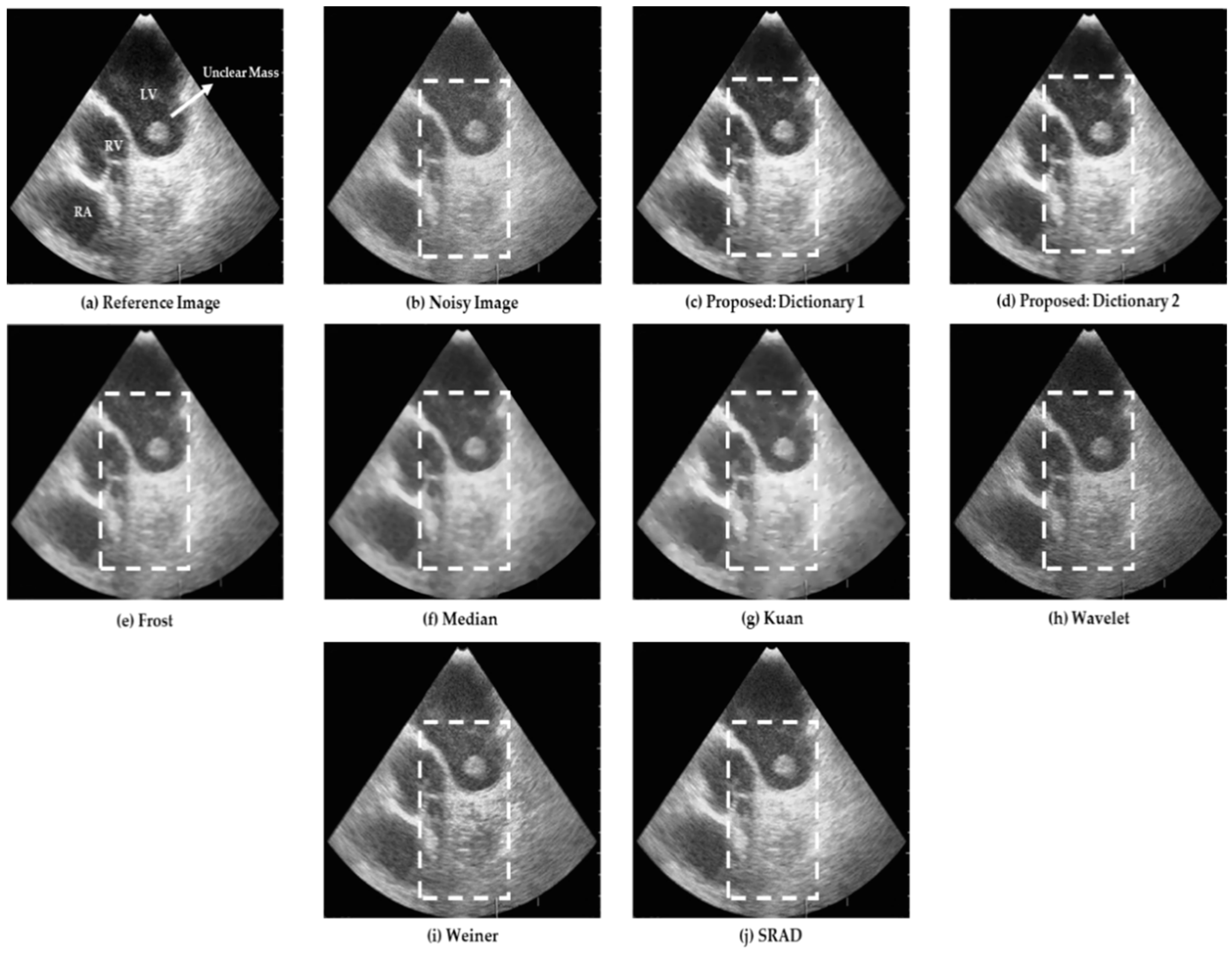
The experiments presented above were performed on ultrasound liver images, and the performance compared with conventional methods. However, our algorithm can also be utilized for a wide range of ultrasound images. To prove this, we conducted experiments on a real thrombus (blood clot) image with a left ventricular mass [56]. The visual assessment was performed using the proposed technique and the results compared to those obtained by various other algorithms. The reference image size was 256 × 256 pixels in order to fit our proposed model. The data were obtained from an open medical imaging dataset on GitHub [57]. The ultrasound image along with a marked note are shown in Figure 9a. The dashed white box in Figure 9b–j indicate regions of the ventricular mass. The thrombus data-set results presented in Figure 9h–j show that the wavelet, Weiner, and SRAD filters performed very poorly in noise reduction. The difference can be seen from the white note marked on the right atrium of the reference ultrasound image in Figure 9a. Figure 9e–g shows that Frost, median, and Kuan reduces speckle but tends to over-smooth the image, which leads to the loss of a distinctive feature of the unclear mass. Among all the methods, Figure 9c,d show good results for the SR-based on learned dictionaries 1 and 2. Several details are well preserved and the speckle noise is reduced efficiently. Figure 10 shows the zoomed sub-images of Figure 9 to observe a clear visualization of the despeckled images. The red box highlights the texture details in the noisy image and the filtered image for a comparative visual assessment. It can be noted that from the Frost, Median, and Kuan filtered data displayed in Figure 10d–f, an unclear mass (blood clot) and texture feature are blurred and over smoothed. Figure 10h,i show that the Weiner and SRAD filters are not much more effective on speckle reduction. These filters also greatly reduce the contrast, making images more indistinguishable from the background. This effect is especially noticeable in the case of the Wavelet filter as shown in Figure 10g. It was found that the anatomical structure was more clearly visible in Figure 10b,c obtained using the SR framework, where the speckle is reduced around the unclear mass without removing its features such as edges and texture. These results were comparatively better than those of Figure 10d–i of the standard despeckling methods. Thus, the proposed algorithm has various advantages for use in CAD systems based on image analysis, such as segmentation and edge detection. Future work will include extensive laboratory and clinical testing on diseased and healthy subjects for a more rigorous validation of the system. In conclusion, our approach reconstructs the detailed information in real ultrasound images, not only by preserving edge information but also by eliminating artifacts and reducing speckle noise.
5. Conclusions
In this paper, we presented a method that reconstructed ultrasound images by suppressing multiplicative speckle noise using the SR framework. The proposed method utilizes an enhanced homomorphic filter, TV regularization, and sparse prior over two learned dictionaries. In addition, the KSVD algorithm is used to train the two dictionaries—one trained with a set of reference ultrasound image patches and another trained with the speckled image patches. Both training options were tested with the synthetic images and various clinical ultrasound images. The experimental results obtained for different noise levels proved superior to those of other standard denoising methods. The results also show that the two modified dictionaries performed well with sparse and TV regularization terms. Overall, the proposed SR framework reconstructs the image signals by removing speckle noise while preserving the texture and yielding a smoother image than conventional methods without eliminating edges.
Author Contributions
M.Y.J. and H.N.L. formulated and designed the experiments; M.Y.J. performed the experiments and analyzed the data; M.Y.J. wrote the manuscript; H.N.L. made revisions to the manuscript and supervised the research work.
Funding
This work was supported by a National Research Foundation of Korea (NRF) grant provided by the Korean government (MSIP) [NRF-2018R1A2A1A19018665].
Conflicts of Interest
The authors declare no conflict of interest.
References
- Szabo, T.L. Diagnostic Ultrasound Imaging: Inside Out; Academic Press Series in Biomedical Engineering; Elsevier Academic Press: New York, NY, USA, 2004; p. 549. ISBN 0-12-680145-2. [Google Scholar]
- Martial, B.; Cachar, D. Acquire real-time RF digital ultrasound data from a commercial scanner. Electron. J. Tech. Accoust. 2007, 3, 16. [Google Scholar]
- Lee, H.; Chen, Y.P.P. Image based computer aided diagnosis system for cancer detection. Expert Syst. Appl. 2015, 42, 5356–5365. [Google Scholar] [CrossRef]
- Jabarulla, M.Y.; Lee, H.N. Computer aided diagnostic system for ultrasound liver images: A systematic review. Optik 2017, 140, 1114–1126. [Google Scholar] [CrossRef]
- Zanotel, M.; Bednarova, I.; Londero, V.; Linda, A.; Lorenzon, M.; Girometti, R.; Zuiani, C. Automated breast ultrasound: Basic principles and emerging clinical applications. Radiol. Med. 2018, 123, 1–12. [Google Scholar] [CrossRef] [PubMed]
- Acharya, U.R.; Koh, J.E.W.; Hagiwara, Y.; Tan, J.H.; Gertych, A.; Vijayananthan, A.; Yaakup, N.A.; Abdullah, B.J.J.; Fabell, M.K.B.M.; Yeong, C.H. Automated diagnosis of focal liver lesions using bidirectional empirical mode decomposition features. Comput. Biol. Med. 2017, 94, 11–18. [Google Scholar] [CrossRef] [PubMed]
- Grazioli, L.; Ambrosini, R.; Frittoli, B.; Grazioli, M.; Morone, M. Primary benign liver lesions: Benign focal liver lesions can origin from all kind of liver cells: Hepatocytes, mesenchymal and cholangiocellular line. Eur. J. Radiol. 2017, 26, 378–398. [Google Scholar] [CrossRef] [PubMed]
- Burckhart, C.B. Speckle in ultrasound B-mode scans. IEEE Trans. Sonics Ultrason. 1978, 25, 1–6. [Google Scholar] [CrossRef]
- Narayanan, S. A view on despeckling in ultrasound imaging. Int. J. Signal Process. Image Process. Pattern Recognit. 2009, 2, 85–98. [Google Scholar]
- Lopes, A.; Touzi, R.; Nezry, E. Adaptive Speckle Filters and Scene Heterogeneity. IEEE Trans. Geosci. Remote Sens. 1990, 28, 992–1000. [Google Scholar] [CrossRef]
- Lee, J.S. Digital image enhancement and noise filtering by use of local statistics. IEEE Trans. Pattern Anal. Mach. Intell. 1980, 2, 165–168. [Google Scholar] [CrossRef] [PubMed]
- Gonzalez, R.C.; Woods, R.E. Digital Image Processing, 3rd ed.; Pearson Education, Inc.: London, UK, 2008; ISBN 0-13-168728-x978-0-13-168728-8. [Google Scholar]
- Goldstein, J.S.; Reed, I.S.; Scharf, L.L. A multistage representation of the Wiener filter based on orthogonal projections. IEEE Trans. Inf. Theory 1998, 44, 2943–2959. [Google Scholar] [CrossRef]
- Kuan, D.T.; Sawchuk, A.A.; Strand, T.C.; Chavel, P. Adaptive noise smoothing filter for images with signal-dependent noise. IEEE Trans. Pattern Anal. Mach. Intell. 1985, 7, 165–177. [Google Scholar] [CrossRef] [PubMed]
- Simon, P.; Patrick, H. Median Filtering in Constant Time. IEEE Trans. Image Process. 2007, 16, 2389–2394. [Google Scholar]
- Achim, A.; Bezerianos, A.; Tsakalides, P. Novel Bayesian multiscale method for speckle removal in medical ultrasound images. IEEE Trans. Med. Imaging 2001, 20, 772–783. [Google Scholar] [CrossRef] [PubMed]
- Chen, Z.J.; Chen, C.H.Y. Efficient statistical modeling of wavelet coefficients for image denoising. Int. J. Wavelets Multiresolut. Inf. Process. 2009, 7, 629–641. [Google Scholar] [CrossRef]
- Vishwa, A.; Sharma, S. Modified method for denoising the ultrasound images by wavelet thresholding. Int. J. Intell. Syst. Appl. 2012, 4, 25. [Google Scholar] [CrossRef]
- Shen, Y.; Liu, Q.; Lou, S.; Hou, Y.L. Wavelet-Based Total Variation and Nonlocal Similarity Model for Image Denoising. IEEE Signal Process. Lett. 2017, 24, 877–881. [Google Scholar] [CrossRef]
- Donoho, D.L. De-noising by soft-thresholding. IEEE Trans. Inf. Theory 1995, 41, 613–627. [Google Scholar] [CrossRef]
- Matsuyama, E.; Tsai, D.-Y.; Lee, Y.; Tsurumaki, M.; Takahashi, N.; Watanabe, H.; Chen, H.-M. A modified undecimated discrete wavelet transform based approach to mammographic image denoising. J. Digit. Imaging 2013, 26, 748–758. [Google Scholar] [CrossRef] [PubMed]
- Kim, Y.S. Improvement of ultrasound image based on wavelet transform: Speckle reduction and edge enhancement. SPIE Med. Imaging 2005, 5747, 1085–1092. [Google Scholar]
- Chambolle, A. An algorithm for total variation minimizations and applications. J. Math. Imaging Vis. 2004, 10, 89–97. [Google Scholar]
- Rudin, L.I.; Osher, S.; Fatemi, E. Nonlinear total variation based noise removal algorithms. Phys. D Nonlinear Phenom. 1992, 60, 259–268. [Google Scholar] [CrossRef]
- Perona, P.; Malik, J. Scale-space and edge detection using anisotropic diffusion. IEEE Trans. Pattern Anal. Mach. Intell. 1990, 12, 629–639. [Google Scholar] [CrossRef]
- Chao, S.M.; Tsai, D.M. An improved anisotropic diffusion model for detail and edge-preserving smoothing. Pattern Recognit. Lett. 2010, 31, 2012–2023. [Google Scholar] [CrossRef]
- Tschumperle, D.; Deriche, R. Vector-valued image regularization with PDEs: A common framework for different applications. IEEE Trans. Pattern Anal. Mach. Intell. 2005, 27, 506–517. [Google Scholar] [CrossRef] [PubMed]
- Zhao, Y.; Yang, J. Hyperspectral image denoising via sparse representation and low-rank constraint. IEEE Trans. Geosci. Remote Sens. 2015, 53, 296–308. [Google Scholar] [CrossRef]
- Elad, M.; Aharon, M. Image denoising via sparse and redundant representations over learned dictionaries in wavelet domain. IEEE Trans. Image Process. 2006, 15, 754–758. [Google Scholar] [CrossRef]
- Deka, B.; Bora, P.K. Removal of correlated speckle noise using sparse and overcomplete representations. Biomed. Signal Process. Control 2013, 8, 520–533. [Google Scholar] [CrossRef]
- Fan, J.; Wu, Y.; Li, M.; Liang, W.; Zhang, Q. SAR Image Registration Using Multiscale Image Patch Features with Sparse Representation. Biomed. Signal Process. Control 2017, 10, 1483–1493. [Google Scholar] [CrossRef]
- Wright, J.; Ma, Y.; Mairal, J.; Sapiro, G.; Huang, T.S.; Yan, S. Sparse representation for computer vision and pattern recognition. Proc. IEEE 2010, 98, 1031–1044. [Google Scholar] [CrossRef]
- Bruckstein, M.E.A.M.; Donoho, D.L.; Elad, M. From sparse solutions of systems of equations to sparse modeling of signals and images. SIAM Rev. 2009, 51, 34–81. [Google Scholar] [CrossRef]
- Li, S.; Wang, G.; Zhao, X. Multiplicative noise removal via adaptive learned dictionaries and TV regularization. Digit. Signal Process. 2016, 50, 218–228. [Google Scholar]
- Liu, K.; Tan, J.; Su, B. An Adaptive Image Denoising Model Based on Tikhonov and TV Regularizations. Adv. Multimed. 2014, 2014, 934834. [Google Scholar] [CrossRef]
- Aharon, M.; Elad, M.; Bruckstein, A.M. The K-SVD: An algorithm for designing of overcomplete dictionaries for sparse representations. IEEE Trans. Signal Process. 2006, 54, 4311–4322. [Google Scholar] [CrossRef]
- Tay, P.C.; Garson, C.D.; Acton, S.T.; Hossack, J.A. Ultrasound despeckling for contrast enhancement. IEEE Trans. Image Process. 2010, 19, 1847–1860. [Google Scholar] [CrossRef] [PubMed]
- Joel, T.; Sivakumar, R. An extensive review on Despeckling of medical ultrasound images using various transformation techniques. Appl. Acoust. 2018, 138, 18–27. [Google Scholar] [CrossRef]
- Youngjian, Y.; Acton, S.T. Speckle reducing anisotropic diffusion. IEEE Trans. Image Process. 2002, 11, 1260–1270. [Google Scholar] [CrossRef] [PubMed]
- Hussain, S.A.; Gorashi, S.M. Image Denoising based on Spatial/Wavelet Filter using Hybrid Thresholding Function. Int. J. Comput. Appl. 2012, 42, 5–13. [Google Scholar]
- Aubert, G.; Aujol, J.-F. A variational approach to removing multiplicative noise. SIAM J. Appl. Math. 2008, 68, 925–946. [Google Scholar] [CrossRef]
- Buades, A.; Coll, B.; Morel, J.M. A review of image denoising algorithms, with a new one. Multiscale Model. Simul. 2005, 4, 490–530. [Google Scholar] [CrossRef]
- Gilboa, S.O.G. Nonlocal operators with applications to image processing. SIAM J. Multiscale Model. Simul. 2008, 7, 1005–1028. [Google Scholar] [CrossRef]
- Cai, T.T.; Wang, L. Orthogonal matching pursuit for sparse signal recovery with noise. IEEE Trans. Inf. Theory 2011, 57, 4680–4688. [Google Scholar] [CrossRef]
- Deka, B.; Bora, P.K. Despeckling of medical ultrasound images using sparse representation. In Proceedings of the 2010 International Conference Signal Processing and Communications (SPCOM), Bangalore, India, 18–21 July 2010. ISSN 2165-0608. [Google Scholar]
- Cobbold, R.S.C. Foundations of Biomedical Ultrasound; Oxford University Press: Oxford, UK, 2007. [Google Scholar]
- Yahya, N.; Kamel, N.S.; Malik, A.S. Subspace-based technique for speckle noise reduction in ultrasound images. Biomed. Eng. Online 2014, 13, 154. [Google Scholar] [CrossRef] [PubMed]
- Arsenault, H.H.; Levesque, M. Combined homomorphic and local-statistics processing for restoration of images degraded by signal-dependent noise. Appl. Opt. 1984, 23, 845–850. [Google Scholar] [CrossRef] [PubMed]
- Xie, H.; Pierce, L.E.; Ulaby, F.T. Statistical properties of logarithmically transformed speckle. IEEE Trans. Geosci. Remote Sens. 2002, 40, 721–727. [Google Scholar] [CrossRef]
- Candes, E.; Candes, E.; Romberg, J.; Romberg, J. l1-Magic: Recovery of Sparse Signals via Convex Programming; Caltech: Pasadena, CA, USA, 2005; pp. 1–19. [Google Scholar]
- Afonso, M.V.; Bioucas-Dias, J.M.; Figueiredo, M.A.T. An augmented Lagrangian approach to the constrained optimization formulation of imaging inverse problems. IEEE Trans. Image Process. 2011, 20, 681–695. [Google Scholar] [CrossRef] [PubMed]
- Davis, G.; Mallat, S.G.; Avellaneda, M. Adaptive greedy approximations. Constr. Approx. 1997, 13, 57–98. [Google Scholar] [CrossRef]
- Xiang, F.; Wang, Z. Split Bregman iteration solution for sparse optimization in image restoration. Optik 2014, 125, 5635–5640. [Google Scholar] [CrossRef]
- Wang, Z.; Bovik, A.; Sheikh, H.; Simoncelli, E. Image quality assessment: From error visibility to structural similarity. IEEE Trans. Image Process. 2004, 4, 600–612. [Google Scholar] [CrossRef]
- Shepp, L.; Logan, F. The Fourier reconstruction of a head section. IEEE Trans. Nucl. Sci. 1974, 21, 21–43. [Google Scholar] [CrossRef]
- Llach, F. Hypercoagulability, renal vein thrombosis, and other thrombotic complications of nephrotic syndrome. Kidney Int. 1985, 3, 429–439. [Google Scholar] [CrossRef]
- GitHub. Available online: https://github.com/sfikas/medical-imaging-datasets (accessed on 1 May 2018).
Figure 1.
Flow diagram of the enhanced homomorphic filter. FFT: fast Fourier transform; IFFT inverse fast Fourier transform.
Figure 1.
Flow diagram of the enhanced homomorphic filter. FFT: fast Fourier transform; IFFT inverse fast Fourier transform.
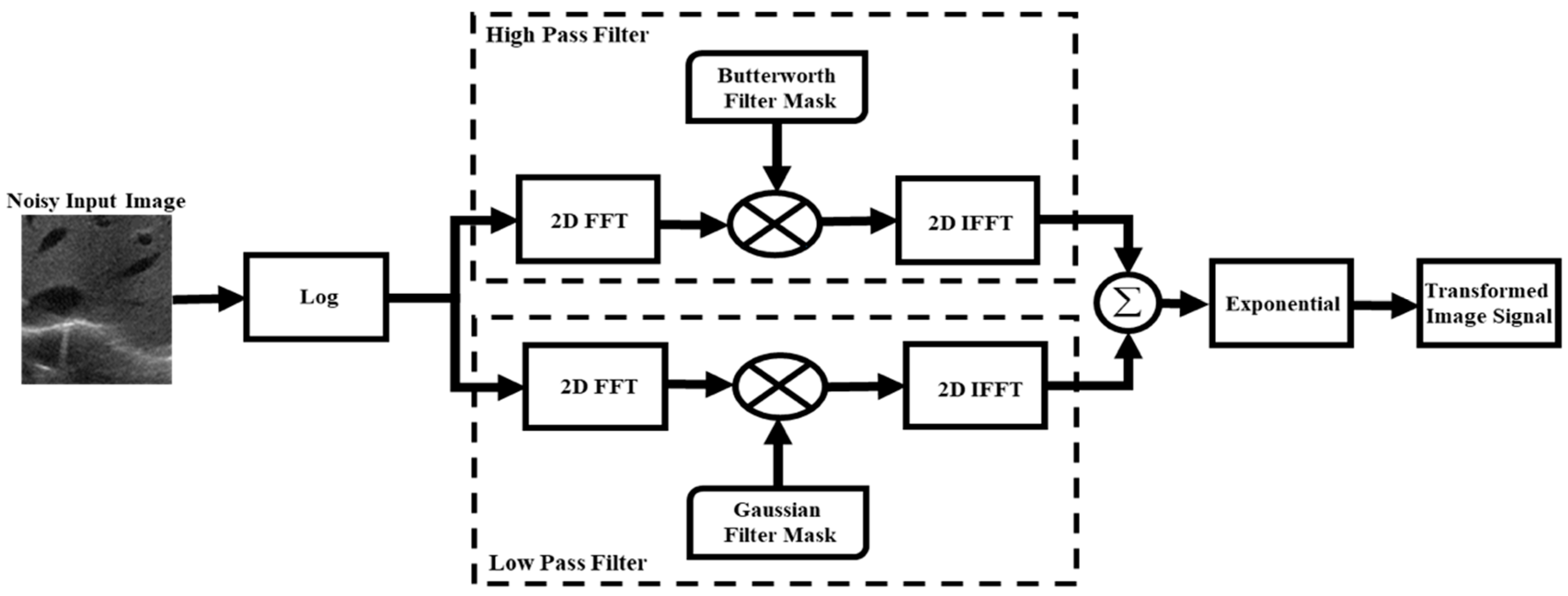
Figure 2.
(a) Noisy ultrasound image; (b) Butterworth high-pass (BW-HP) filtered image; (c) Gaussian low pass (GLP) filtered image; and (d) transformed output of ultrasound noisy image.
Figure 2.
(a) Noisy ultrasound image; (b) Butterworth high-pass (BW-HP) filtered image; (c) Gaussian low pass (GLP) filtered image; and (d) transformed output of ultrasound noisy image.

Figure 3.
Proposed despeckle model for an ultrasound image. KSVD: K-singular value decomposition.
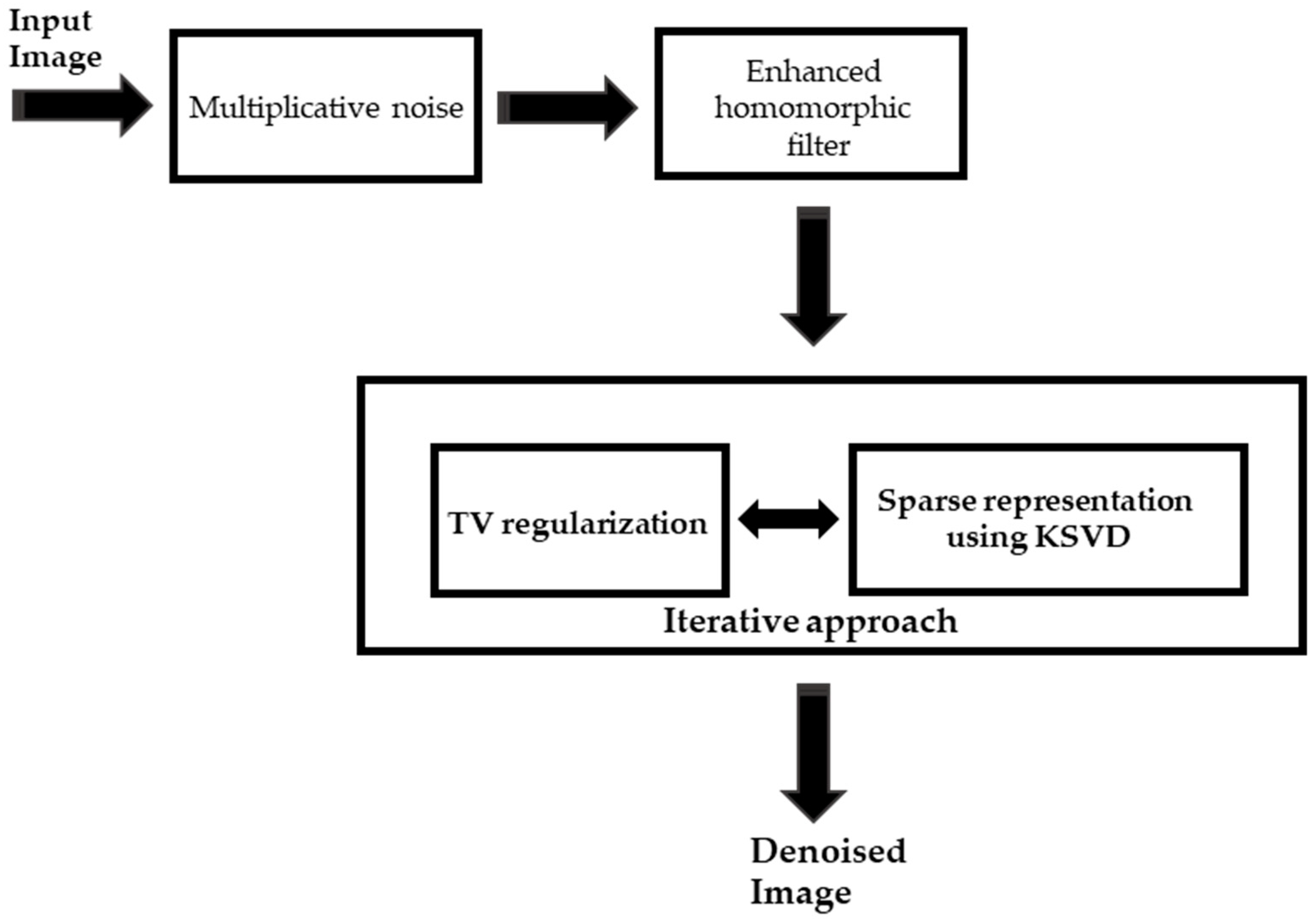
Figure 4.
(a) Original image; (b) noisy image. Results of the proposed method with (c) Dictionary 1 and (d) Dictionary 2; Results of the (e) Frost; (f) wavelet; (g) Kuan; (h) median; (i) Weiner; and (j) speckle reducing anisotropic diffusion (SRAD) filters.
Figure 4.
(a) Original image; (b) noisy image. Results of the proposed method with (c) Dictionary 1 and (d) Dictionary 2; Results of the (e) Frost; (f) wavelet; (g) Kuan; (h) median; (i) Weiner; and (j) speckle reducing anisotropic diffusion (SRAD) filters.
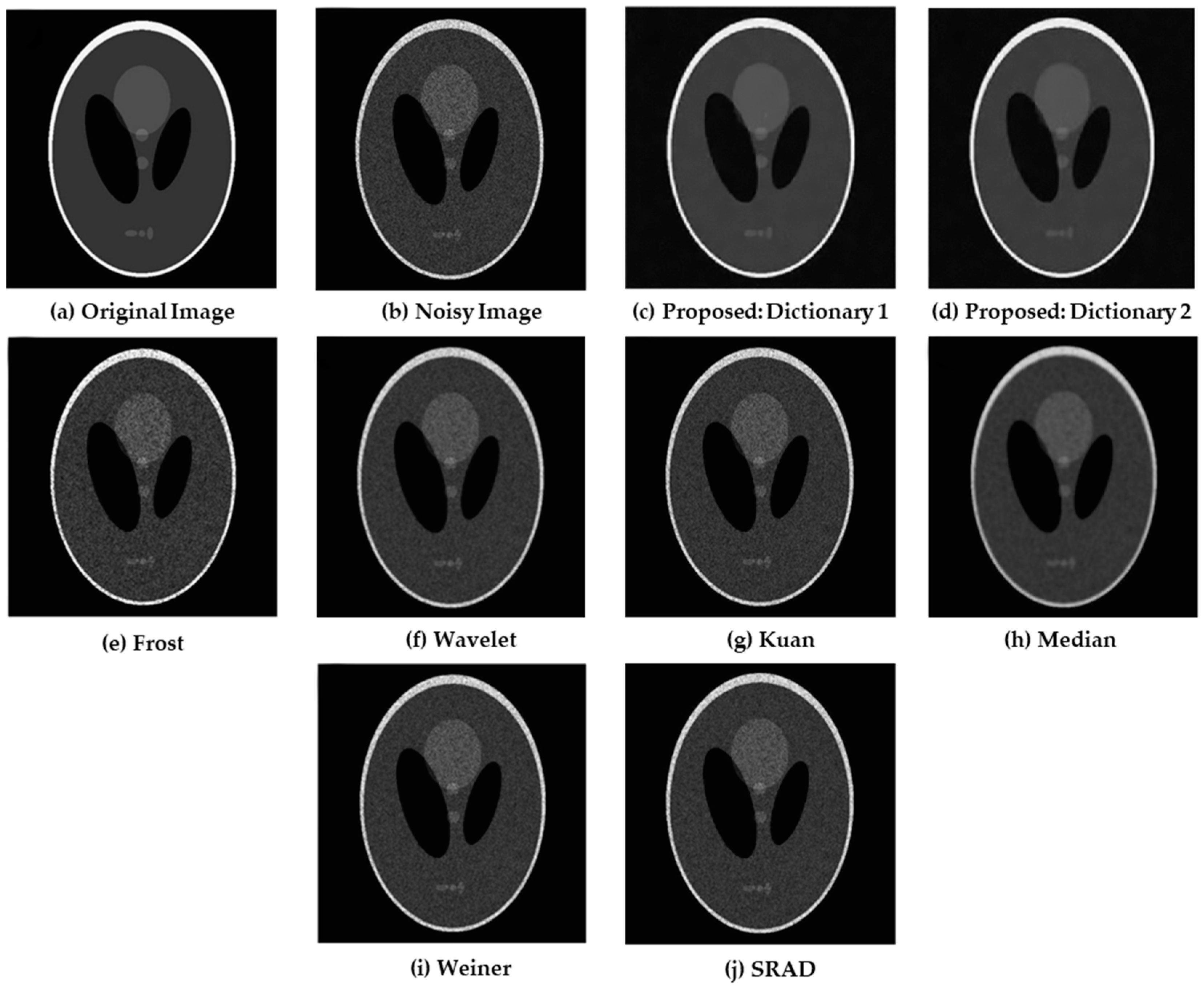
Figure 5.
The random collections of 16 × 16 atoms (K = 256) of trained dictionary from (a) a reference set of 3245 ultrasound images and (b) a noisy image.
Figure 5.
The random collections of 16 × 16 atoms (K = 256) of trained dictionary from (a) a reference set of 3245 ultrasound images and (b) a noisy image.

Figure 6.
Reconstruction of liver right lobe images. (a) Original ultrasound image; (b) Speckled ultrasound image (PSNR = 28.148 dB); Images reconstructed using (c) Dictionary 1 (PSNR = 35.033 dB) and (d) Dictionary 2 (PSNR = 35.537 dB).
Figure 6.
Reconstruction of liver right lobe images. (a) Original ultrasound image; (b) Speckled ultrasound image (PSNR = 28.148 dB); Images reconstructed using (c) Dictionary 1 (PSNR = 35.033 dB) and (d) Dictionary 2 (PSNR = 35.537 dB).

Figure 7.
Despeckled results obtained for the ultrasound liver dataset using a linear transducer with a frequency of 8 MHz. The red and the green boxes highlight the differences observed from the noisy and filtered images. (a) Speckled image and results yielded by the proposed method using (b) Dictionary 1 and (c) Dictionary 2 as well as results using the (d) Frost; (e) median; (f) Kuan; (g) wavelet; (h) Weiner; and (i) SRAD filters.
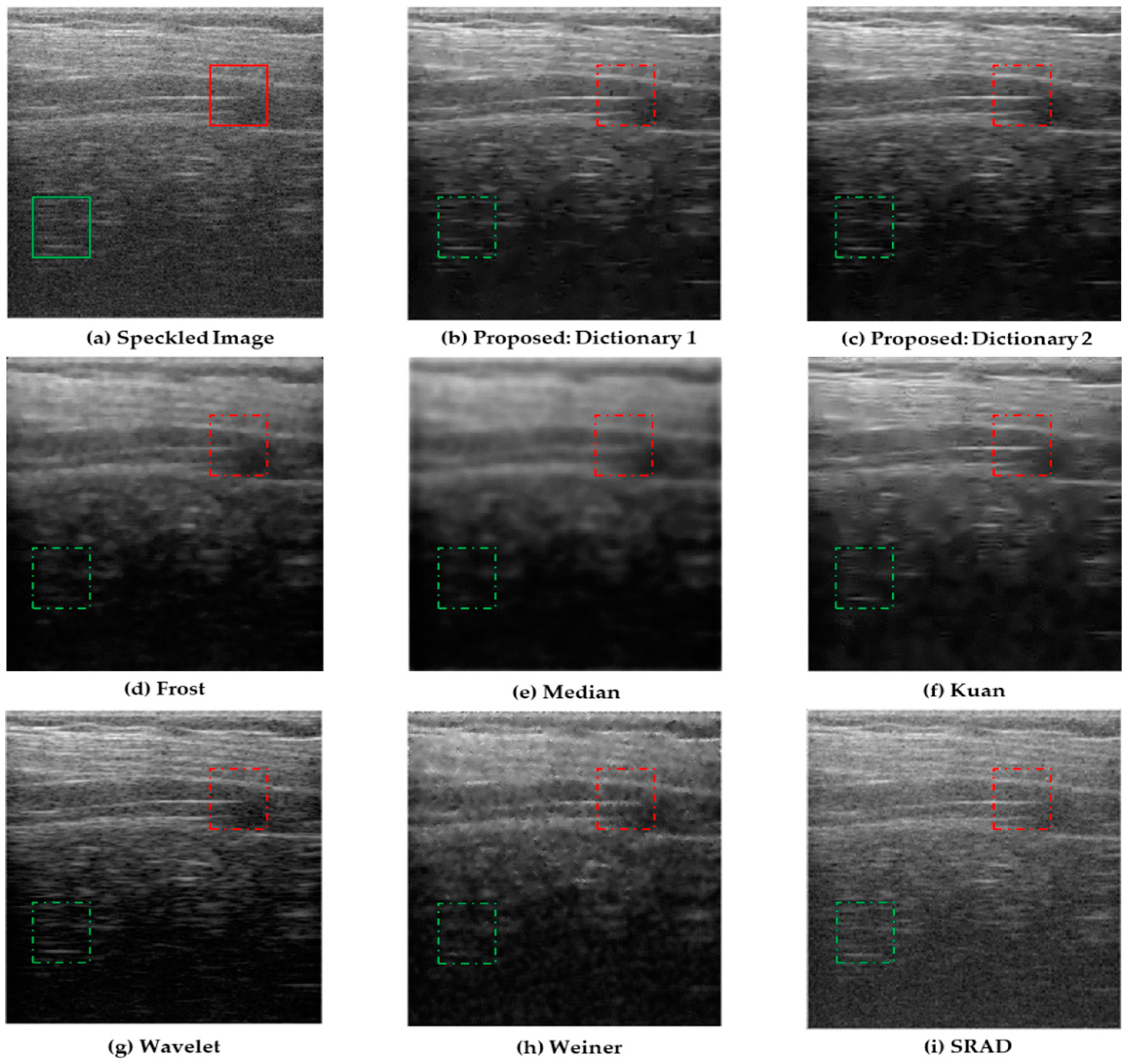
Figure 8.
Comparison of PSNRs obtained by different methods. SRAD: speckle reducing anisotropic diffusion.
Figure 8.
Comparison of PSNRs obtained by different methods. SRAD: speckle reducing anisotropic diffusion.

Figure 9.
(a) Ultrasound image of the thrombus in the left ventricle. LV: left ventricle, RA: right atrium and RV: right ventricle and (b) noisy image. Despeckled ultrasound images of proposed method using (c) Dictionary 1 and (d) Dictionary 2. Results using the (e) Frost, (f) median, (g) Kuan, (h) wavelet, (i) Weiner, and (j) SRAD filters. The dashed white box indicates the region of image showing visual enhancement owing to despeckling.

Figure 10.
(a) Zoomed sub-image of noisy thrombus ultrasound images. The red boxes highlight texture details of images for visual assessment. Results of proposed method using (b) Dictionary 1 and (c) Dictionary 2. Results using the (d) Frost; (e) median; (f) Kuan; (g) wavelet; (h) Weiner; and (i) SRAD filters.

Table 1.
Peak signal-to-noise ratio (PSNR) and mean structural similarity (MSSIM) for the synthetic images for = 10.
Table 1.
Peak signal-to-noise ratio (PSNR) and mean structural similarity (MSSIM) for the synthetic images for = 10.
| Models | PSNR (dB) | MSSIM |
|---|---|---|
| Noise image | 32.113 | 0.727 |
| Frost | 32.466 | 0.768 |
| Wavelet | 33.214 | 0.801 |
| Kuan | 32.895 | 0.794 |
| Median | 34.597 | 0.839 |
| SRAD | 33.434 | 0.827 |
| Weiner | 33.782 | 0.834 |
| Proposed: Dictionary 1 | 36.862 | 0.953 |
| Proposed: Dictionary 2 | 37.044 | 0.967 |
Table 2.
PSNR and MSSIM for the ultrasound liver image for = 15.
| Models | PSNR (dB) | MSSIM |
|---|---|---|
| Frost | 28.966 | 0.822 |
| Median | 25.497 | 0.659 |
| Wavelet | 27.772 | 0.782 |
| SRAD | 28.766 | 0.813 |
| Kuan | 28.279 | 0.801 |
| Weiner | 29.218 | 0.834 |
| Proposed: Dictionary 1 | 30.334 | 0.901 |
| Proposed: Dictionary 2 | 30.807 | 0.926 |
© 2018 by the authors. Licensee MDPI, Basel, Switzerland. This article is an open access article distributed under the terms and conditions of the Creative Commons Attribution (CC BY) license (http://creativecommons.org/licenses/by/4.0/).
Share and Cite
MDPI and ACS Style
Jabarulla, M.Y.; Lee, H.-N. Speckle Reduction on Ultrasound Liver Images Based on a Sparse Representation over a Learned Dictionary. Appl. Sci. 2018, 8, 903. https://doi.org/10.3390/app8060903
AMA Style
Jabarulla MY, Lee H-N. Speckle Reduction on Ultrasound Liver Images Based on a Sparse Representation over a Learned Dictionary. Applied Sciences. 2018; 8(6):903. https://doi.org/10.3390/app8060903
Chicago/Turabian StyleJabarulla, Mohamed Yaseen, and Heung-No Lee. 2018. "Speckle Reduction on Ultrasound Liver Images Based on a Sparse Representation over a Learned Dictionary" Applied Sciences 8, no. 6: 903. https://doi.org/10.3390/app8060903
Note that from the first issue of 2016, this journal uses article numbers instead of page numbers. See further details here.