Article

Artificial Neural Networks in Coordinated Control of Multiple Hovercrafts with Unmodeled Terms

1
Department of Computer and Information Science, University of Macau, Taipa 999078, Macau, China
2
School of Computer Science, North China University of Technology, Beijing 100144, China
*
Authors to whom correspondence should be addressed.
Appl. Sci. 2018, 8(6), 862; https://doi.org/10.3390/app8060862
Submission received: 17 April 2018 / Revised: 16 May 2018 / Accepted: 22 May 2018 / Published: 24 May 2018
(This article belongs to the Special Issue Multi-Agent Systems)

Abstract

:
In this paper, the problem of coordinated control of multiple hovercrafts is addressed. For a single hovercraft, by using the backstepping technique, a nonlinear controller is proposed, where Radial Basis Function Neural Networks (RBFNNs) are adopted to approximate unmodeled terms. Despite the application of RBFNNs, integral terms are introduced, improving the robustness of controller. As a result, global uniformly ultimate boundedness is achieved. Regarding the communication topology, two different directed graphs are chosen under the assumption that there are no delays when they communicate with each other. In order to testify the performance of the proposed strategy, simulation results are presented, showing that vehicles can move forward in a specific formation pattern and RBFNNs are able to approximate unmodeled terms.

1. Introduction

In recent years, Wireless Sensor Networks (WSNs) have attracted growing interests from researchers, because they have merits, compared with traditional networking solutions, such as reliability, flexibility, and an ease of deployment, that enable their use in a wide range of varied application scenarios [1]. They can be applied to track moving objects, to monitor special areas so as to trigger alarm systems when some dangerous signals are detected, etc. As the eyes and ears of the IoT, WSNs can work as bridges to build connections between the real-world and the digital-world. In light of this promising application scenario, this paper mainly focuses on a case study of mobile WSNs, where a group of hovercrafts equipped with specific sensors are chosen as test platforms. The objective is to enable them to move around and interact with the physical environment [2] and thus execute a mission of mapping, searching, and monitoring in a specific area.
Coordinated control of a fleet of hovercrafts is challenging, especially when we take into account their complex dynamic models. Until now, for a single surface vehicle, many research results have been reported. For example, a linear fuzzy-PID controller was proposed in [3]. Compared with the ordinary PID controller, the proposed controller therein performs better in term of improving settling time and reducing overshoot of the control signal. However, their works just consider the kinematic models of the vehicle without considering the dynamic models, which is not realistic in real operation scenarios. Another weakness of the linear controller is that it usually achieves local stability, e.g., [4], where velocity and position controllers were developed based on a linearized system, which is controllable only when the angular velocity is nonzero. Considering the limitations of linear controllers, in [5,6], nonlinear controllers for underactuated ships were designed, and global asymptotic stability is achieved. In [7], a nonlinear Lyapunov-based tracking controller was presented, and it was able to exponentially stabilize the position tracking error to a neighborhood of the origin that can be made arbitrarily small. A method of incorporating multiobjective controller selection into a closed-loop control system was presented in [8], where the authors designed three controllers so as to capture three “behaviors” representative of typical maneuvers that would be performed in a port environment. However, none of the works mentioned above consider disturbances and unmodeled terms of the vehicle. In order to ensure that the vehicle is robust to external disturbances, in [9], two controllers with application to a surface vehicle (named Qboat) and a hovercraft were proposed, and the authors designed disturbance estimators to estimate external constant disturbances. The disadvantage of this control strategy is that they did not consider unmodeled terms involved in the dynamic model of the vehicle. Considering this constraint, an estimator was developed in [10], where a fuzzy system was used to approximate unknown kinetics. A fault tolerant tracking controller was designed in [11] for a surface vessel. In addition, a self-constructing adaptive robust fuzzy neural control scheme for tracking surface vessels was proposed in [12], where simulation results were shown to testify the efficiency of the proposed method therein.
With respect to coordinated control strategy for multiple vehicles, many authors have presented their own approaches. In [13], a cooperative path following methodology was proposed under the assumption that the communication among a group of fully-actuated surface vehicles is undirected and continuous. A coordinated path following with a switching communication topology was designed in [14], while a null-space-based behavioral control technique was proposed in [15,16]. In [17,18,19], a leader–follower control strategy was presented. In [20], an adaptive coordinate tracking control problem for a fleet of nonholonomic chained systems was discussed under the assumption that the desired trajectory is available only to part of the neighbors. The reader is also referred to [21] for more results about multi-vehicle control approaches.
Inspired and motived by those works mentioned above, in this paper, we first develop a controller that is able to drive a single hovercraft to the neighborhood of a desired smooth path, where a Radial Basis Function Neural Network (RBFNN) is applied to approximate unmodeled dynamic terms of the vehicle while integral error terms are introduced, thus improving the robust performance of the controller. It is relevant to point out that all elements of the estimation weight matrix are always bounded through the use of a smooth projection function. We also derive a consensus strategy to make sure the desire paths progress in a specific formation. In order to validate the effectiveness of the proposed strategy, simulation results are presented.
The rest of the paper is organized as follows: Section 2 presents robot modeling, graph theory, RBFNNs, and coordinated control problem. A single controller is proposed in Section 3, while Section 4 devises a consensus strategy. Simulation results are given in Section 5 to validate the performance of the proposed approach herein. At last, Section 6 summarizes our work and describes the future work.

2. Problem Formulation

2.1. Vehicle Modeling

We first define a global coordinate frame { U } and a body frame { B } as shown in Figure 1. The kinematic equations of the vehicle are written as
p ˙ = R v
ψ ˙ = ω
where p ˙ = [ x , y ] T denotes the coordinates of its center of mass, v = [ u , v ] T represents linear velocity, ψ is the orientation of the vehicle, and its angular velocity is represented by ω . Moreover, the rotation matrix R ( ψ ) is given by
R ( ψ ) = cos ( ψ ) sin ( ψ ) sin ( ψ ) cos ( ψ ) .
Its dynamic equations are
v ˙ = S ( ω ) v + m 1 T n 1 + Δ v
ω ˙ = J 1 ω + J 1 τ + Δ ω
where S ( ω ) is a skew symmetric matrix, given by
S ( ω ) = 0 ω ω 0 .
n 1 = [ 1 , 0 ] T , m and J denote the car’s mass and rotational inertial, respectively. The force used to make the car move forward is denoted by T, and τ represents the torque that can steer the vehicle. Unmodeled dynamic terms are represented by Δ v and Δ ω . For more details about modeling surface vehicles, the reader is referred to [22].

2.2. Graph Theory

In this paper, G = G ( V , E ) denotes a directed graph that can be used to model the interaction communication topology among mobile robots. The graph G consists of a finite set V = { 1 , 2 , , n } of n vehicles and a finite set E of m pairs of vertices V i j = { i , j } E . If V i j belongs to E , then i and j are said to be adjacent. A graph from i to j is a sequence of distinct vertices starting with i and ending with j such that consecutive vertices are adjacent. In this case, V i j also represents a directional communication link from agent i to agent j. The adjacency matrix of the graph G is denoted by A = [ a i j ] R n × n , which is a square matrix where a i j equals to one if { j , i } E and zero otherwise. Moreover, the Laplacian matrix L is defined as L = D A , where the degree matrix D = [ d i j ] R n × n of the graph G is a diagonal matrix and d i j equals the number of adjacent vertices of vertex i.

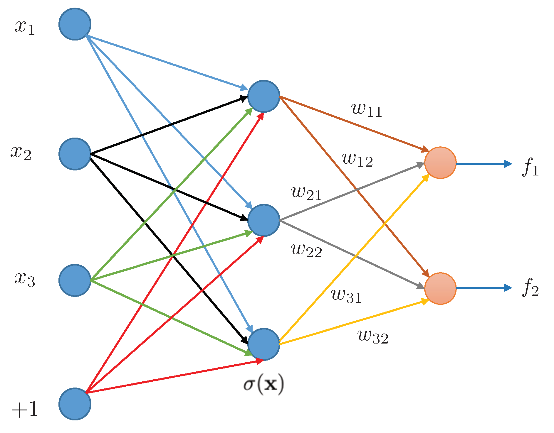
2.3. Radial Basis Function Neural Networks

Radial Basis Function Neural Networks (RBFNNs) can be used to approximate the unmodeled nonlinear dynamic terms due to their universal approximation capability [23]. For any unknown smooth function f ( x ) : R n R m can be approximated by RBFNNs in the following form, given by
f ^ ( x ) = W T σ ( x )
where x Ω R n , Ω is a compact set. The adjustable weight matrix with n neurons is denoted by W R n × m under the assumption that it is a bounded matrix, that is
W W max .
It is important to point out that here when we say matrix x R m × n is smaller than or equal to x max R m × n , we mean all elements of x are smaller than or equal to their corresponding elements of x max R m × n . Moreover, σ ( x ) is the basis function vector and σ i ( x i ) = exp ( ( x i μ i ) T ( x i μ i ) / c i 2 ) , i = 1 , 2 , , n denotes its component, μ i is the center of the receptive field, and c i represents the width of the Gaussian function. Moreover, it is relevant to point out that, in order to achieve better approximate results, we should make the neuron number n large enough and choose the parameters properly. Going back to the smooth function f ( x ) mentioned above, there is an ideal weight W d such that
f ( x ) = W d T σ ( x ) + ϵ ( x )
where ϵ ( x ) denotes the approximation error and satisfies | | ϵ ( x ) | | ϵ max , where ϵ max is a positive number. It is noted that W d is an “artificial” quantity for the purpose of mathematic analysis, in the process of controller design, we need to estimate it [24]. A simple RBFNNs is given by Figure 2.

2.4. Problem Statement

Now we can state our problem: Through designing a controller for each robot and proposing consensus strategies for their corresponding desired paths, we want a group of mobile robots to move forward in a specific formation pattern; that is,
(1)
for an individual vehicle, | | p p d | | δ , where δ is an arbitrarily small constant value;
(2)
for a group of n desired paths, γ i γ j 0 and γ ˙ i γ ˙ d 0 , where agent j is the neighbor of agent i, γ ˙ d represents the desired value of γ ˙ i , which is a known value.

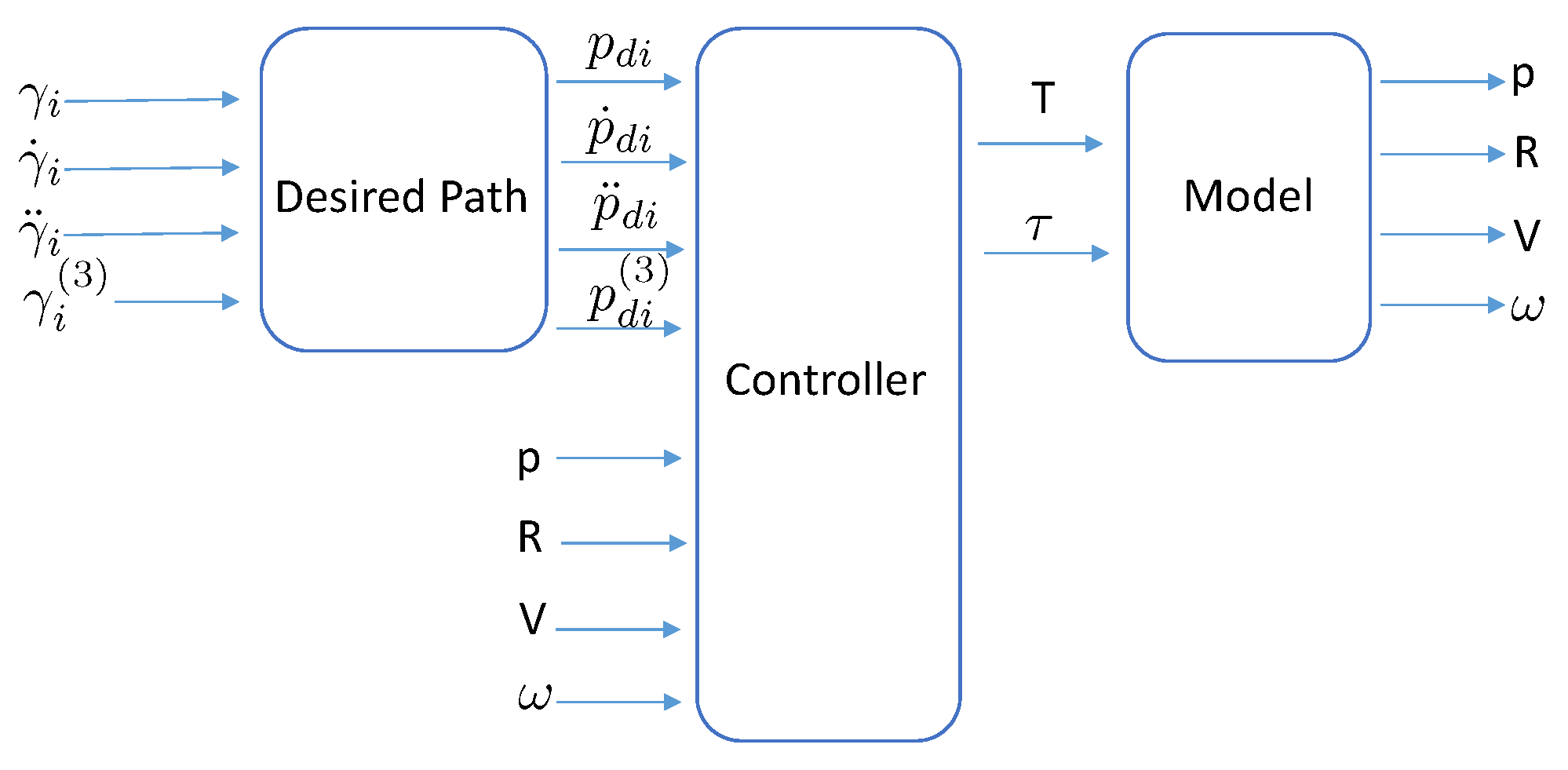
3. Controller Design

Following the works of [7] and [9], we define the position error in the body frame as
e 1 = R T ( p p d )
where R = R ( ψ ) denotes the rotation matrix. The time derivative of e 1 yields
e ˙ 1 = S ( ω ) e 1 + v R T p ˙ d .
Define our first Lyapunov function as
V 1 = 1 2 e 1 T e 1
and compute its time derivative, we have
V ˙ 1 = α 1 + e 1 T ( v R T p ˙ d + k 1 e 1 )
where α 1 = k 1 e 1 T e 1 is positive definite, and k 1 denotes gain, which is a positive value.
In order to continue to use the backstepping technique, a second error term is defined as
e 2 = v R T p ˙ d + k 1 e 1 η ,
and its integral term
e 2 n = 0 t e 2 d t
where η = [ η 1 , η 2 ] T , η 1 0 is a constant vector. Define our second Lyapunov function as
V 2 = V 1 + 1 2 e 2 T e 2 + 1 2 e 2 n T e 2 n ,
and its time derivative yields
V ˙ 2 = α 2 + e 1 T η + e 2 T ( S ( ω ) η + m 1 T n 1 R T p ¨ d + k 1 ( e 2 k 1 e 1 + η ) + k 2 e 2 + Δ v + e 2 n )
where α 2 = k 1 e 1 T e 1 + k 2 e T e 2 , which is positive definite, and k 2 is a positive number. It is relevant to point out that e 2 n is introduced to eliminate the external slow-varying disturbances that act on the dynamic of the linear velocity v . Moreover, notice that we do not know Δ v , thereby we use RBFNNs mentioned before to approximate it, given by
Δ v = W d 1 T σ ( x 1 ) + ϵ 1 ( x 1 )
where x 1 = [ 1 , v T ] T R 3 . Moreover, notice that
S ( ω ) η + m 1 T n 1 = N I
where
N = m 1 η 2 0 η 1 . I = [ T , ω ] T .
Rewrite Equation (17), and we have
V ˙ 2 = α 2 + e 1 T η + e 2 T N I + β + W d 1 T σ ( x 1 ) + e 2 T ϵ 1 ( x 1 )
where β = R T p ¨ d + k 1 ( e 2 k 1 e 1 + η ) + k 2 e 2 + e 2 n .
Now, we can define our third Lyapunov function as
V 3 = V 2 + 1 2 W ˜ d 1 T Γ 1 1 W ˜ d 1
where W ˜ d 1 = W d W ^ d 1 denotes the estimation error, Γ 1 = ( λ 11 , a n d λ 12 ) is a matrix, where λ 11 and λ 12 are positive values. Compute the time derivative of V 3 , and one obtains
V ˙ 3 = α 2 + e 1 T η + e 2 T ϵ 1 ( x 1 ) + e 2 T N I + β + W ^ d 1 T σ ( x 1 ) + e 2 T W ˜ d 1 T σ ( x 1 ) W ˜ d 1 T Γ 1 1 W ^ ˙ d 1 .
Therefore, we choose our desired input I d as
I d = N 1 β + W ^ d 1 T σ ( x 1 ) ,
and thereby our first controller T is chosen as
T = n 1 T I d .
Correspondingly, the desired angular velocity is
ω d = n 2 T I d
where n 2 = [ 0 , 1 ] T .
Notice that, if the updated law for W ^ ˙ d 1 is set as
W ^ ˙ d 1 = Γ 1 σ ( x 1 ) e 2 T ,
we cannot ensure that it is bounded by W max . To solve this problem, a projection operator, which is Lipschitz continuous [25], is applied in our case, which is given by
proj ( ρ , ^ ) = ρ if   Θ ( ^ ) 0 ρ if   Θ ( ^ ) 0   and   Θ ^ ( ^ ) ρ 0 ( 1 Θ ( ^ ) ) ρ if   Θ ( ^ ) > 0   and   Θ ^ ( ^ ) ρ > 0
where
Θ ( ^ ) = ^ 2 max 2 ϵ 2 + 2 ϵ max 2 , Θ ^ ( ^ ) = Θ ( ^ ) ^ ,
with the following condition: if ^ ˙ = p r o j ( ρ , ^ ) and ^ ( t 0 ) max , then
(1)
^ max + ϵ , 0 t < ;
(2)
proj ( ρ , ^ ) is Lipschitz continuous;
(3)
| proj ( ρ , ^ ) | | ρ | ;
(4)
˜ proj ( ρ , ^ ) ˜ ρ , where ˜ = ^ .
Therefore, to make sure all elements of W ^ d 1 are upper-bounded, the update law for W ^ ˙ d 1 is finally set as
W ^ ˙ d 1 = Γ 1 proj σ ( x 1 ) e 2 , W ^ d 1 .
To keep using the backstepping technique, we define a new error term
e 3 = ω ω d ,
and its corresponding integral term
e 3 n = 0 t e 3 d t .
Then, we define a new Lyapunov function as
V 4 = V 3 + 1 2 e 3 T e 3 + 1 2 e 3 n T e 3 n .
Compute its time derivatives, substitute Equation (29) into Equation (24), and combine the 4th property of projector ( ˜ proj ( ρ , ^ ) ˜ ρ ) , and one obtains
V ˙ 4 α 3 + e 1 T η + e 2 T ϵ 1 ( x 1 ) + e 3 T ( n 2 T N T e 2 1 J τ + n 2 T N 1 ( β ˙ + W ^ ˙ d 1 σ ( x 1 ) + W ^ d 1 σ ˙ ( x 1 ) ) + k 3 e 3 + e 3 n + Δ ω )
where α 3 = α 2 + k 3 e 3 T e 3 0 , k 3 > 0 . However, it is noted that both β ˙ and σ ˙ ( x 1 ) contain unmodeled term Δ v , so we need to separate Δ v out from β ˙ and σ ˙ ( x 1 ) . After that, we can use RBFNNs to estimate it. Similar to Δ ω , we also need to approximate it. This is given by,
Δ v = W d 2 T σ ( x 2 ) + ϵ 2 ( x 2 )
Δ ω = W d 3 T σ ( x 3 ) + ϵ 3 ( x 3 )
where x 2 = [ 1 , v T ] T R 3 and x 3 = [ 1 , v T , ω ] T R 4 .
Now we define our last Lyapunov function as
V 5 = V 4 + 1 2 tr W ˜ d 2 T Γ 2 1 W ˜ d 2 + 1 2 tr W ˜ d 3 T Γ 3 1 W ˜ d 3
where W ˜ d 2 = W d W ^ d 2 , W ˜ d 3 = W d W ^ d 3 , Γ 2 = diag ( λ 21 , λ 22 ) , and Γ 3 = diag ( λ 31 , λ 32 ) are positive definite gain matrices. Then, we compute the time derivative of V 5 as
V ˙ 5 α 3 + e 1 T η + e 2 T ϵ 1 ( x 1 ) + e 3 T ( n 2 T M ) ϵ 2 ( x 2 ) + e 3 T ϵ 3 ( x 3 ) + e 3 T ( n 2 T N T e 2 + k 3 e 3 τ J n 2 T I ˙ ^ d n 2 T M W ^ 2 d T σ ( x 2 ) + W ^ 3 d T σ ( x 3 ) + e 3 n ) + e 3 T n 2 T M W ˜ 2 d T σ ( x 2 ) + e 3 T W ˜ 3 T σ ( x 3 ) tr W ˜ d 2 T Γ 2 1 W ^ ˙ d 2 tr W ˜ d 3 T Γ 3 1 W ^ ˙ d 3
where
I ˙ ^ d = β ˙ ^ + W ^ ˙ d 1 σ ( x 1 ) + W ^ d 1 σ ˙ ^ ( x 1 )
and
M = N 1 W ^ d 1 T G + ( k 1 + k 2 ) N 1
with G = [ 0 2 × 1 T , n 1 σ ( n 1 T v ) , a n d n 1 σ ( n 2 T v ) ] T . Then, we define our second control law, torque, as
τ = J ( n 2 T I ˙ ^ d + n 2 T N T e 2 + k 3 e 3 + n 2 T M W ^ d 2 T σ ( x 2 ) + W ^ d 3 T σ ( x 3 ) + e 3 n ) ,
and estimate laws for W ^ ˙ d 2 and W ^ ˙ d 3
W ^ ˙ d 2 = Γ 2 proj σ ( x 2 ) ( n 2 T M ) e 3 T W ^ d 2 ,
W ^ ˙ d 3 = Γ 3 proj σ ( x 3 ) e 3 T , W ^ d 3 .
Substitute Equation (40)–(42) into Equation (37), one obtains
V ˙ 5 α 3 + e 1 T η + e 2 T ϵ 1 ( x 1 ) + e 3 T ( n 2 T M ) ϵ 2 ( x 2 ) + e 3 T ϵ 3 ( x 3 ) .
where α 3 = k 1 e 1 T e 1 + k 2 e 2 T e 2 + k 3 e 3 T e 3 .

3.1. Stability Analysis

Theorem 1.
For a single mobile robot, by applying control laws, Equations (24) and (40), and updated laws, Equation (29), Equation (41), and Equation (42), for any large initial position, the robot will converge to the neighborhood of its corresponding desired path p d ( γ ) , whose partial derivatives with respect to γ are all bounded. As a consequence, global uniformly ultimately boundedness is achieved.
Proof. 
Let’s go back to Equation (43). Rewrite it, and we obtain
V ˙ 5 X T K X + X T ρ | X | T k min | X | + | ρ |
where X = [ e 1 T , e 2 T , e 3 T ] , k min is the smallest eigenvalue of K = ( k 1 , k 2 , k 3 ) , and ρ = [ η T , ϵ 1 ( x 1 ) T , ( n 2 T M ) ϵ 2 ( x 2 ) , ϵ 3 ( x 3 ) ] T , which is bounded due to the fact that | | ϵ i ( x ) | | ϵ max , and the upper bound of ρ is
ρ max = [ η T , ϵ 1 max ( x 1 ) T , ( n 2 T M ) ϵ 2 max ( x 2 ) , ϵ 3 max ( x 3 ) ] T .
Thereby, we can obtain that V ˙ 5 is negative for | | X | | | | ρ max / k min | | , which can be made as small as possible by tuning the value of k min . As a result, the system is uniformly ultimate bounded, global uniformly ultimate boundedness is achieved. ☐

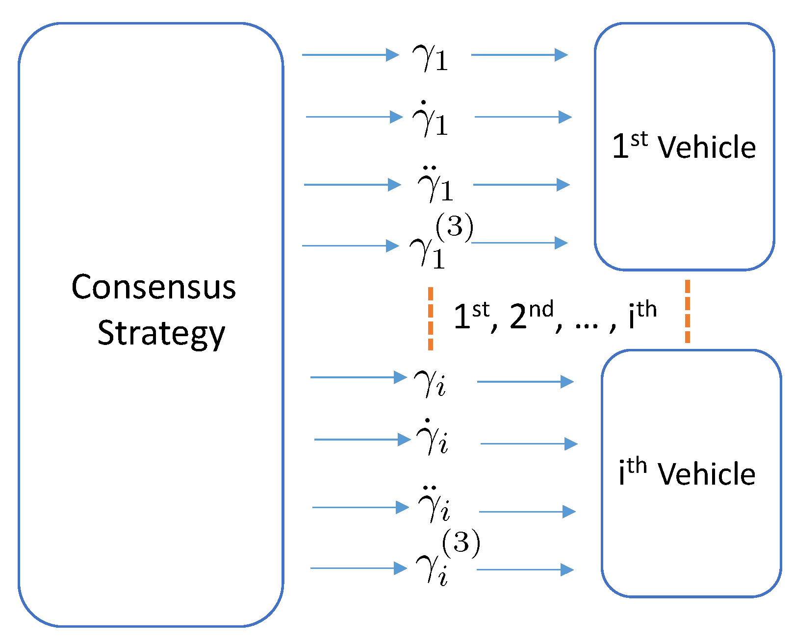
4. Consensus Strategy

Building upon the work of [14], the proposed solution is given by
γ ˙ i = v d 1 a 1 j N i ( γ i γ j ) + z i
z ˙ i = a 2 z i + a 3 j N i ( γ i γ j )
where a 1 , a 2 , a n d a 3 are positive numbers, and v d denotes the desired value of γ ˙ i . It is relevant to point out that z i can be viewed as an auxiliary state that helps n paths to reach consensus.

4.1. Stability Analysis

Theorem 2.
For a group of n desired paths p d ( γ i ) ( i = 1 , 2 , , n ) , by applying Equations (46) and (47), γ i γ j and γ ˙ i γ ˙ d converge to zero.
Proof. 
We first choose Laplacian matrix L , and define the coordinate error as
Γ e = L Λ
where Λ = [ γ i ] n × 1 . Rewrite Equations (46) and (47), and one obtains
Γ ˙ e = A 1 L Γ e + L Z ,
Z ˙ = A 2 Z + A 3 Γ e ,
where A i = ( a i ) , ( i = 1 , 2 , 3 ) is a positive definite matrix. Define x = [ Γ e , Z ] T , and rewrite Equations (49) and (50), and we have
x ˙ = A x
where
A = A 1 L L A 3 A 2 .
In order to ensure that Equation (51) is stable, we need to guarantee that all the eigenvalues of A have negative or zero real parts and all the Jordan blocks corresponding to eigenvalues with zero real parts are 1 × 1 . We consider n agents, where
L = 0 0 0 0 0 1 1 0 0 0 0 1 1 0 0 0 0 0 1 1 n × n .
For the sake of saving space, here we just present the eigenvalues of A directly, they are λ 1 , λ 2 , λ 3 , and λ 4 , and their corresponding multiplicities are 1, 1, n 1 , and n 1 , with
λ 1 = 0
λ 2 = a 2
λ 3 = ( a 1 + a 2 ) / 2 + a 1 2 + a 2 2 2 a 1 a 2 + 4 a 3 / 2
λ 4 = ( a 1 + a 2 ) / 2 a 1 2 + a 2 2 2 a 1 a 2 + 4 a 3 / 2 .
Choosing a 1 , a 2 , a n d a 3 properly, we can guarantee that λ 2 , λ 3 , and λ 4 are negative-definite. Moreover, we also have that the Jordan block corresponding to λ 1 is 1 × 1 . As a consequence, Equation (51) is stable [26]. ☐
To summarize, a fleet of n desired paths can progress in a specific formation, while each individual mobile robot converges to the neighborhood of its corresponding desired path. As a result, all those robots can move forward in a specific formation.

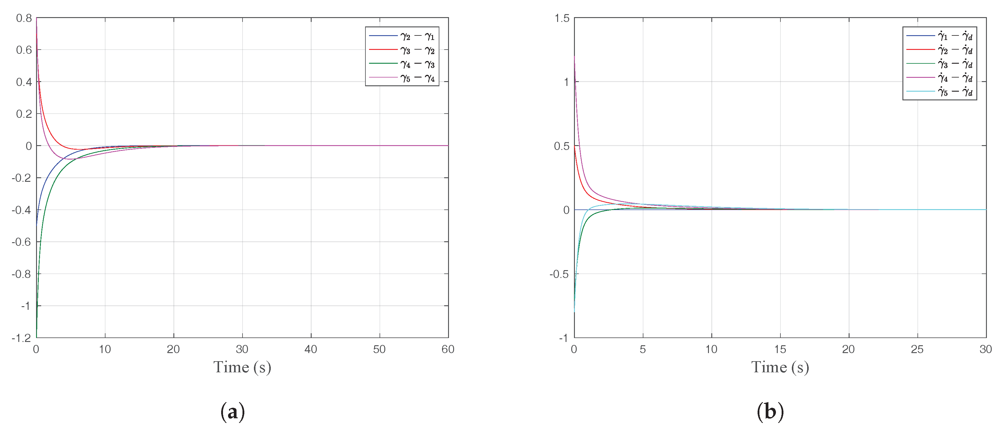
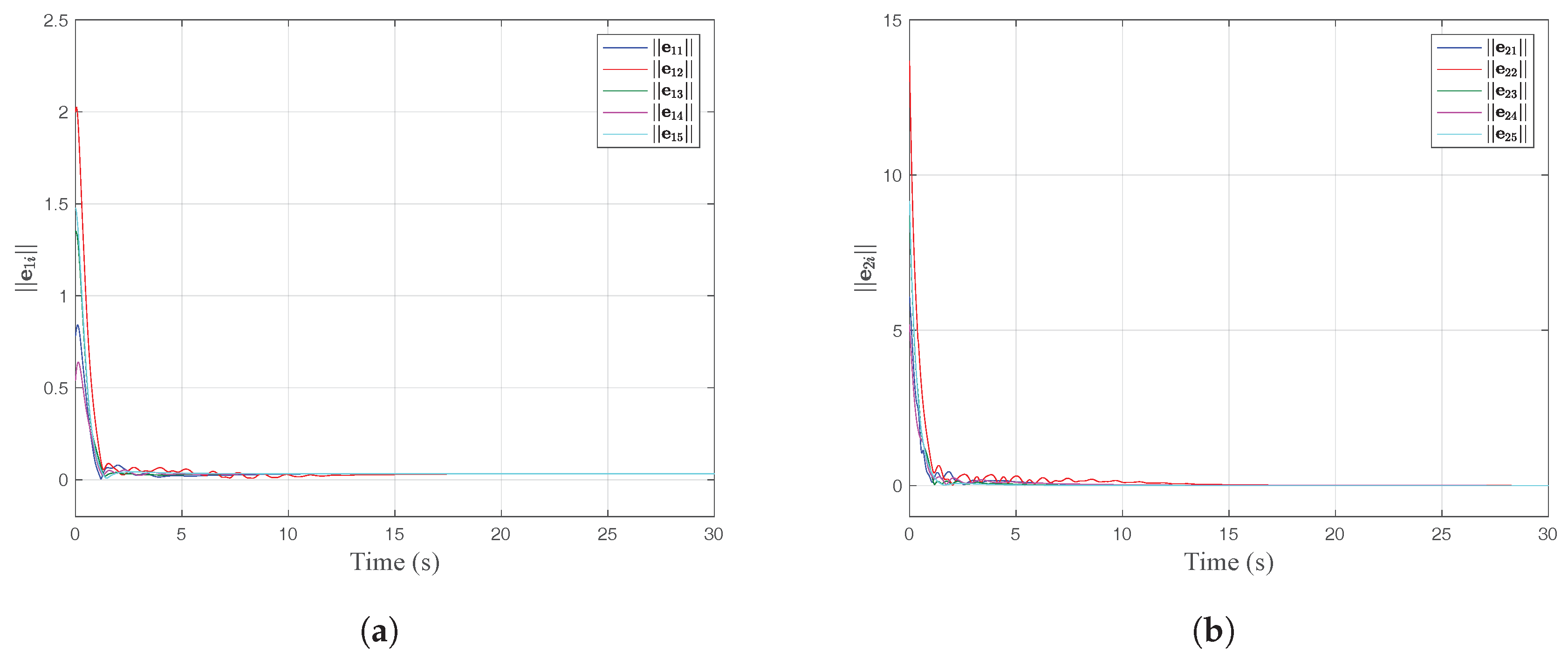
5. Simulation Results

In this section, we present simulation results with two different communication graphs including a cascade-directed communication graph (CDCG) and a parallel-directed communication graph (PDCG). Figure 3 and Figure 4 show the sketches of the control blocks in Simulink/Matlab.

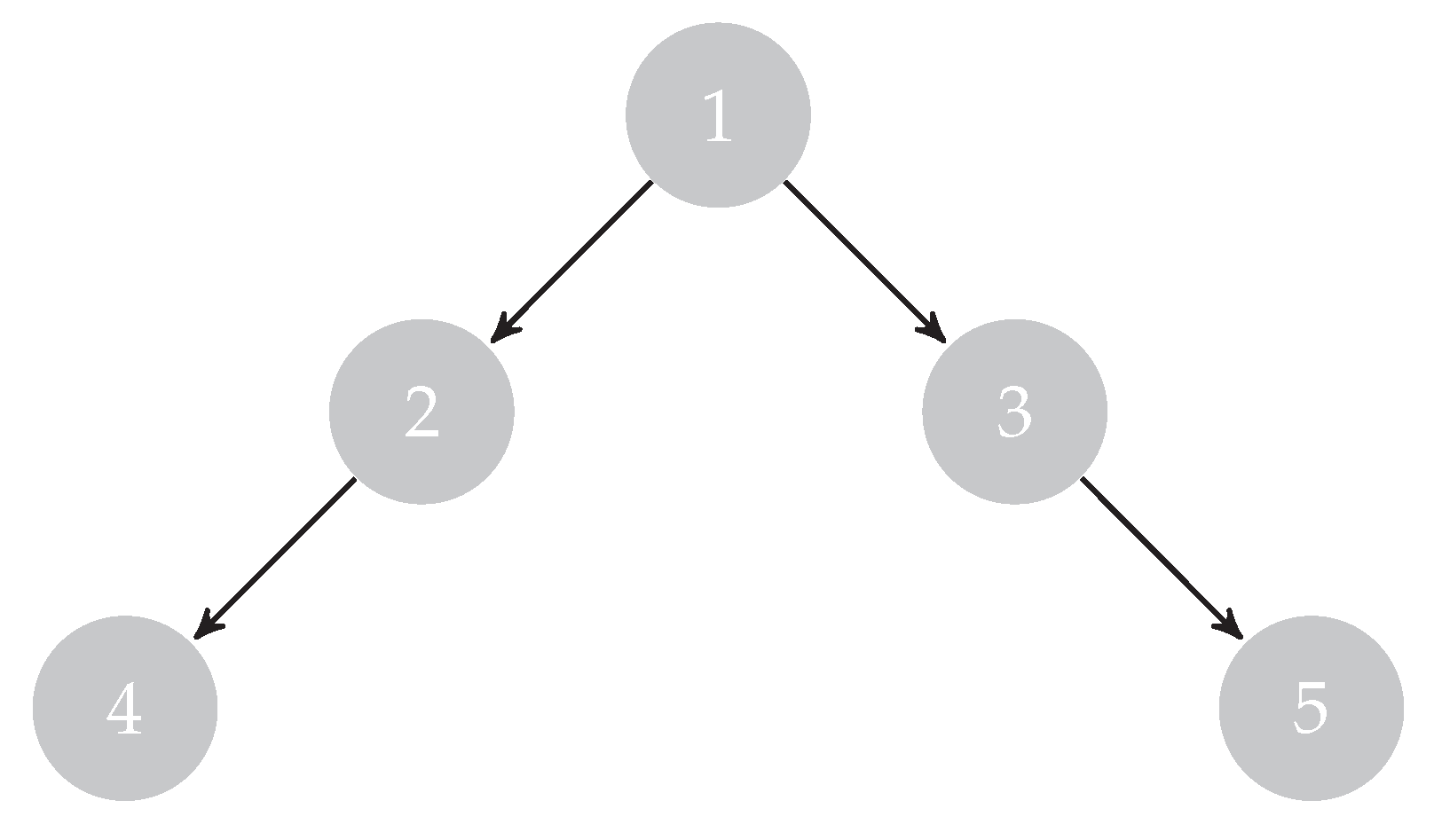
5.1. The Cascade-Directed Communication Graph

The CDCG used in this study is shown in Figure 5, where agent 1 can be viewed as the leader. Its corresponding Laplacian matrix L 1 is
L 1 = 0 0 0 0 0 1 1 0 0 0 0 1 1 0 0 0 0 1 1 0 0 0 0 1 1 .
The desired paths are defined as
p d i ( γ i ) = R i cos ( γ i ) sin ( γ i ) ( m )
where R i = 6 i , ( i = 1 , 2 , , 5 ) denotes the radius of the circle, and unmodeled terms Δ V and Δ ω are denoted by [ 0.1 u 2 + 0.01 u v , 0.01 u v + 0.1 v 2 ] T and 0.01 u v + 0.05 u ω + 0.01 v ω , respectively. The parameters used herein are as follows: m = 0.6 , J = 0.1 , c i = 2 , a 1 = 1 , a 2 = 2 , a 3 = 1 , k 1 = 6 , k 2 = 3 , k 3 = 2 , Γ 1 = ( 0.6 , 0.6 ) , Γ 2 = ( 0.01 , 0.01 ) , Γ 3 = ( 0.022 , 0.022 ) , and η = [ 0.2 , 0 ] T .
Figure 6a shows the actual trajectory of the mobile robots, and we can see that they move forward in a line formation. Moreover, Figure 7a,b display the convergence of | | e 1 i | | and | | e 2 i | | , respectively, showing that all of them converge to the neighborhood of zero. The consensus performances are shown in Figure 8a,b, showing that γ i j = γ i γ j converges to zero, where agent j is the neighbor of agent i. Moreover, we can also see that γ ˙ i converges to the desired value γ ˙ d = 0.5 . It is important to point out that, in this work, we chosen agent 1 as our leader, and this satisfies γ ˙ 1 = γ ˙ d . The approximate performance of RBFNNs can be found in Figure 6b, where the blue lines denote the real values of Δ v and Δ ω , while the red lines represent their estimates Δ ^ v and Δ ^ ω . Thus, both estimates converge to their corresponding real values.

5.2. Parallel Communication Graph

The parallel communication graph is depicted in Figure 9.
In this case, the Laplacian matrix L 2 is
L 2 = 1 1 0 0 0 1 0 1 0 0 0 1 0 1 0 0 0 1 0 1 0 0 0 0 0 .
Moreover, it is noted that the graph presented in Figure 9 can be viewed as the combination of two cascade-directed graphs, where 1 2 4 and 1 3 5 and where agent 1 is the leader whose state is known. The desired paths are as follows:
(1)
1st vehicle:
p d 1 ( γ 1 ) = R 1 cos ( γ 1 ) sin ( γ 1 ) ( m )
(2)
2nd vehicle:
p d 2 ( γ 2 ) = R 2 cos ( γ 2 π / 24 ) sin ( γ 2 ) π / 24 ( m )
(3)
3rd vehicle:
p d 3 ( γ 3 ) = R 3 cos ( γ 3 π / 12 ) sin ( γ 3 π / 12 ) ( m )
(4)
4th vehicle:
p d 4 ( γ 4 ) = R 4 cos ( γ 4 π / 24 ) sin ( γ 4 π / 24 ) ( m )
(5)
5th vehicle:
p d 5 ( γ 5 ) = R 5 cos ( γ 5 π / 12 ) sin ( γ 5 π / 12 ) ( m )
where R 1 = 3 , R 2 = 4 , R 3 = 2 , R 4 = 5 , and R 5 = 1 . Figure 10a displays the actual paths of the robots. From Figure 11a,b, we can obtain that the norm of position errors and linear velocity errors converge to a ball centered at the origin. Moreover, Figure 12a,b show the performance of the consensus strategy introduced herein.
It is interesting to remark that, by using the proposed consensus strategy—Equations (46) and (47)—a consensus is researched if and only if the directed graph has a directed spanning tree [21]. However, in our case, the root must be the leader whose states are known beforehand.

6. Conclusions

In this paper, we mainly focus on designing coordinated control algorithms for multiple agents, where a group of underactuated hovercrafts were chosen as test platforms. In order to testify the efficiency of the devised control strategy, we implemented it by using Simulink/Matlab. Moreover, it is necessary to point out that agents can also be mobile robots, unmanned air vehicles, etc. For a single vehicle, we used RBFNNs to approximate unmodeled terms and introduce integral terms, which can improve the robustness of the controller. For multiple vehicles, we consider directed topology under the assumption that the communication among vehicles are continuous.
With respect to our future works, we plan to (i) use deep neural networks to estimate unmodeled terms so as to enhance the performance of approximation, (ii) build a mathematical model for external disturbance, such as winds, waves, or currents, (iii) take into account time-delays when we develop communication strategy for vehicles, and (iv) propose collision–avoidance algorithms so that we can ensure the operation is safe.

Author Contributions

K.D. and S.F. conceived and designed the experiments; K.D. performed the experiments and wrote the paper; Y.Z. and W.S. provided guidance for this paper.

Acknowledgments

The authors are grateful for financial support from the following research grants: (1) the ‘Nature-Inspired Computing and Metaheuristics Algorithms for Optimizing Data Mining Performance’ grant from the University of Macau (grant no. MYRG2016-00069-FST); the (2) ’Improving the Protein–Ligand Scoring Function for Molecular Docking by Fuzzy Rule-Based Machine Learning Approaches’ grant from the University of Macau (grant no. MYRG2016-00217-FST), and (3) the ‘A Scalable Data Stream Mining Methodology: Stream-based Holistic Analytics and Reasoning in Parallel‘ grant from the FDCT, the Macau Government (grant no. FDCT/126/2014/A3).

Conflicts of Interest

The authors declare no conflict of interest.

References

  1. Rawat, P.; Singh, K.D.; Chaouchi, H.; Bonnin, J.M. Wireless sensor networks: a survey on recent developments and potential synergies. J. Supercomput. 2014, 68, 1–48. [Google Scholar] [CrossRef]
  2. Yick, J.; Mukherjee, B.; Ghosal, D. Wireless sensor network survey. Comput. Netw. 2008, 52, 2292–2330. [Google Scholar] [CrossRef]
  3. Majid, M.H.A.; Arshad, M.R. A Fuzzy Self-Adaptive PID Tracking Control of Autonomous Surface Vehicle. In Proceedings of the IEEE International Conference on Control System, Computing and Engineering, George Town, Malaysia, 27–29 November 2015. [Google Scholar]
  4. Fantoni, I.; Lozano, R.; Mazenc, F.; Pettersen, K.Y. Stabilization of a nonlinear underactuated hovercraft. In Proceedings of the 38th Conference on Decision and Control, Phoenix, AZ, USA, 7–10 December 1999. [Google Scholar]
  5. Do, K.D.; Jiang, Z.P.; Pan, J. Underactuated Ship Global Tracking Under Relaxed Conditions. IEEE Trans. Autom. Control 1999, 47, 1529–1536. [Google Scholar] [CrossRef]
  6. Do, K.D.; Jiang, Z.P.; Pan, J. Universal controllers for stabilization and tracking of underactuated ships. Syst. Control Lett. 2002, 47, 299–317. [Google Scholar] [CrossRef]
  7. Aguiar, A.P.; Cremean, L.; Hespanha, J.P. Position tracking for a nonlinear underactuated hovercraft: Controller design and experimental results. In Proceedings of the 42nd IEEE Conference on Decision and Control, Maui, HI, USA, 9–12 December 2003; Volume 4, pp. 3858–3863. [Google Scholar]
  8. Bertaska, I.R.; Ellenrieder, K.D. Experimental Evaluation of Supervisory Switching Control for Unmanned Surface Vehicle. IEEE J. Ocean. Eng. 2017. [Google Scholar] [CrossRef]
  9. Xie, W. Robust Motion Control of Underactuated Autonomous Surface Craft. Master’s Thesis, University of Macau, Macau, China, 2016. [Google Scholar]
  10. Peng, Z.H.; Wang, J.; Wang, D. Distributed Maneuvering of Autonomous Surface Vehicles Based on Neurodynamic Optimization and Fuzzy Approximation. IEEE Trans. Control Syst. Technol. 2018, 26, 1083–1090. [Google Scholar] [CrossRef]
  11. Chen, X.; Tan, W.W. Tracking control of surface vessel via fault tolerant adaptive backstepping interval type-2 fuzzy control. Ocean Eng. 2013, 26, 97–109. [Google Scholar] [CrossRef]
  12. Wang, N.; Meng, J.E. Self-Constructing Adaptive Robust Fuzzy Neural Tracking Control of Surface Vehicles With Uncertainties and Unknown Disturbances. IEEE Trans. Control Syst. Technol. 2015, 23, 991–1002. [Google Scholar] [CrossRef]
  13. Almeida, J.; Silvestre, C.; Pascoal, A. Cooperative control of multiple surface vessels in the presence of ocean currents and parametric model uncertainty. Int. J. Robust Nonlinear Control 2010, 20, 1549–1565. [Google Scholar] [CrossRef]
  14. Ghabcheloo, R.; Aguiar, A.P.; Pascoal, A.; Silvestre, C.; Kaminer, I.; Hespanha, J.P. Coordinated path-following control of multiple underactuated autonomous vehicles in the presence of communication failures. In Proceedings of the 45th IEEE Conference on Decision Control, San Diego, CA, USA, 13–15 December 2006. [Google Scholar]
  15. Arrichiello, F.; Chiaverini, S.; Fossen, T.I. Formation control of marine surface vessels using the null-space-based behavioral control. In Group Coordination and Cooperative Control. Lecture Notes in Control and Information Science; Springer: Berlin, Germany, 2006; Volume 336. [Google Scholar]
  16. Balch, T.; Arkin, R.C. Behavior-based formation control for multirobot teams. IEEE Trans. Robot. Autom. 1999, 14, 926–939. [Google Scholar] [CrossRef]
  17. Shojaei, K. Leader–follower formation control of underactuated autonomous marine surface vehicles with limited torque. Ocean Eng. 2015, 105, 196–205. [Google Scholar] [CrossRef]
  18. Peng, Z.H.; Wang, D.; Chen, Z.Y.; Hu, X.J.; Lan, W.Y. Adaptive Dynamic Surface Control for Formations of Autonomous Surface Vehicles with Uncertain Dynamics. IEEE Trans. Control Syst. Technol. 2013, 21, 513–520. [Google Scholar] [CrossRef]
  19. Luca, C.; Fabio, M.; Domenico, P.; Mario, T. Leader-follower formation control of nonholonomic mobile robots with input constraints. Automatica 2008, 44, 1343–1349. [Google Scholar]
  20. Wang, Q.; Chen, Z.; Yi, Y. Adaptive coordinated tracking control for multi-robot system with directed communication topology. Int. J. Adv. Rob. Syst. 2017, 14. [Google Scholar] [CrossRef]
  21. Ren, W.; Beard, R. Distributed Consensus in Multi-Vehicle Cooperative Control-Theory and Applications; Springer: Berlin, Germany, 2007. [Google Scholar]
  22. Fossen, T.I. Modeling of Marine Vehicles. In Guidance and Control of Ocean Vehicles; John Wiley & Sons Ltd.: Chichester, UK, 1994; pp. 6–54. ISBN 0-471-94113-1. [Google Scholar]
  23. Wen, G.X.; Chen, P.C.L.; Liu, Y.J.; Liu, Z. Neural-network-based adaptive leader-following consensus control of second-order nonlinear multi-agent systems. IET Control Theory Appl. 2015, 9, 1927–1934. [Google Scholar] [CrossRef]
  24. Wen, G.X.; Chen, P.C.L.; Liu, Y.J.; Liu, Z. Neural Network-Based Adaptive Leader-Following Consensus Control for a Class of Nonlinear Multiagent State-Delay Systems. IEEE Trans. Cybern. 2017, 47, 2151–2160. [Google Scholar] [CrossRef] [PubMed]
  25. Do, K.D. Robust adaptive path following of underactuated ships. Automatic 2004, 40, 929–944. [Google Scholar] [CrossRef]
  26. Hespanha, J.P. Internal or Lyapunov Stability. In Linear Systems Theory; Princeton University Press: Princeton, NJ, USA, 2009; pp. 63–78. ISBN 978-0-691-14021-6. [Google Scholar]
Figure 1. Simple Model of The Vehicle.
Applsci 08 00862 g001
Figure 2. Simple example of RBFNNs.
Applsci 08 00862 g002
Figure 3. Coordinated control block in Simulink/Matlab.
Applsci 08 00862 g003
Figure 4. Control block in Simulink/Matlab for the i-th vehicle.
Applsci 08 00862 g004
Figure 5. A cascade-directed communication graph (CDCG).
Applsci 08 00862 g005
Figure 6. Norm of the position errors and the performance of unmodeled term approximation (CDCG). (a) Norm of the position errors. (b) Performance of unmodeled term approximation.
Applsci 08 00862 g006
Figure 7. Norm of the position and linear velocity errors (CDCG). (a) Norm of the position errors. (b) Norm of the linear velocity errors.
Applsci 08 00862 g007
Figure 8. Performance of γ i γ j and γ ˙ i γ ˙ d , where γ j is the neighbor of γ i (CDCG). (a) Performance of γ i γ j . (b) Performance of γ ˙ i γ ˙ d .
Applsci 08 00862 g008
Figure 9. A parallel-directed communication graph (PDCG).
Applsci 08 00862 g009
Figure 10. Norm of the position errors and performance of unmodeled term approximation (PDCG). (a) Norm of the position errors. (b) Performance of unmodeled term approximation.
Applsci 08 00862 g010
Figure 11. Norm of the position and linear velocity errors (PDCG). (a) Norm of the position errors. (b) Norm of the linear velocity errors.
Applsci 08 00862 g011
Figure 12. Performance of γ i γ j and γ ˙ i γ ˙ d , where γ j is the neighbor of γ i (PDCG). (a) Performance of γ i γ j . (b) Performance of γ ˙ i γ ˙ d .
Applsci 08 00862 g012

