Numerical Analysis of Q-Switched Erbium Ion Doped Fluoride Glass Fiber Laser Operation Including Spontaneous Emission

1
Department of Telecommunications and Teleinformatics, Faculty of Electronics, Wroclaw University of Science and Technology, Wybrzeże Wyspianskiego 27, Wroclaw 50-370, Poland
2
George Green Institute for Electromagnetics Research, The University of Nottingham, University Park, Nottingham NG7-2RD, UK
Appl. Sci. 2018, 8(5), 803; https://doi.org/10.3390/app8050803
Submission received: 25 April 2018
/
Revised: 9 May 2018
/
Accepted: 11 May 2018
/
Published: 16 May 2018
(This article belongs to the Special Issue Rare-Earth Doping for Optical Applications)
Abstract
:Featured Application
Erbium ion doped fluoride glass fiber lasers have many potential applications in medicine, defense and environment monitoring. The software tool developed here can be applied for efficient design and modelling of erbium ion doped fluoride glass fiber lasers. The results presented concern in particular a Q-switched operation of the laser.
Abstract
Partial differential equations are solved to perform a spatiotemporal analysis of Q-switched operation of a fluoride fiber laser doped with erbium ions. A method of lines is applied in order to reduce the partial differential equations to a set of ordinary differential equations. The latter set is then solved using an algorithm designed for a solution of stiff equation problems. A spontaneous emission term is added to equations that model the dynamics of the photon population within the laser cavity for the infrared signal wave. The results show that, without an inclusion of the spontaneous emission term, the correct behavior of the photon population and energy level populations cannot be reproduced.
1. Introduction
Over the last two decades there has been considerable progress in the development of fluoride glass fiber lasers doped with lanthanide ions with operating wavelengths larger than 2500 nm. So far, the longest operating wavelength achieved using fluoride fiber laser technology is 3900 nm, which was realized using liquid nitrogen cooling of ZBLAN fiber doped with holmium ions [1]. At room temperature, the longest operating wavelength achieved so far is 3680 nm [2], which was realized using erbium ion doped ZBLAN fiber and a two pump lasing scheme [3]. The output power under continuous wave (CW) operation erbium ion doped ZBLAN fiber lasers has reached 24 W in a cavity configuration using bulk optics elements [4], whilst in an all fiber, passively cooled configuration, 20 W was reached [5]. The slope efficiency of lanthanide ion doped fluoride fiber lasers has so far reached 73% [6]. Also, fluoride fiber lasers, with a very large wavelength tuning range covering the mid-infrared wavelength range up to 3400 nm, have been realized [7]. Pulsed operation of lanthanide ion fluoride glass fiber lasers has been achieved using both gain switching and Q-switching. The highest average power obtained so far using Q-switching is 12 W [8], whilst the highest peak power is 10 kW [9]. Gain switched dual pump erbium doped fluoride fiber lasers have achieved an operating wavelength of 3550 nm with a peak power of 204 W and a repetition frequency of 15 kHz [10].
The progress in practical realization of lanthanide ion fluoride glass fiber lasers was accompanied by a development of design and modelling tools. Most of the fiber laser models developed thus far rely on solving the rate and propagation equations for the pump and signal waves in the time domain, and rely on the application of the method of characteristics (MOC) [11,12,13,14,15,16,17]. When using MOC, the spatial and temporal step ratio has to remain fixed, to preserve the physical meaning of the results obtained. More recently, an alternative approach has been introduced which relies on the application of the method of lines (FD-MOL) [18], and the concept of the Extended Taylor Series (ETS) [19,20], to derive second order finite difference (FD) approximations for spatial derivatives. In this contribution, FD-MOL is used to model the Q-switched operation of the fluoride glass fiber laser doped with erbium ions. It was shown that inclusion of the spontaneous emission phenomenon is essential for obtaining correct results.
The paper is divided into four sections. After an introduction, the model details are presented in the second section. In the third section, a discussion of the results is provided, which is followed by a concise summary in the last section.
2. Methods
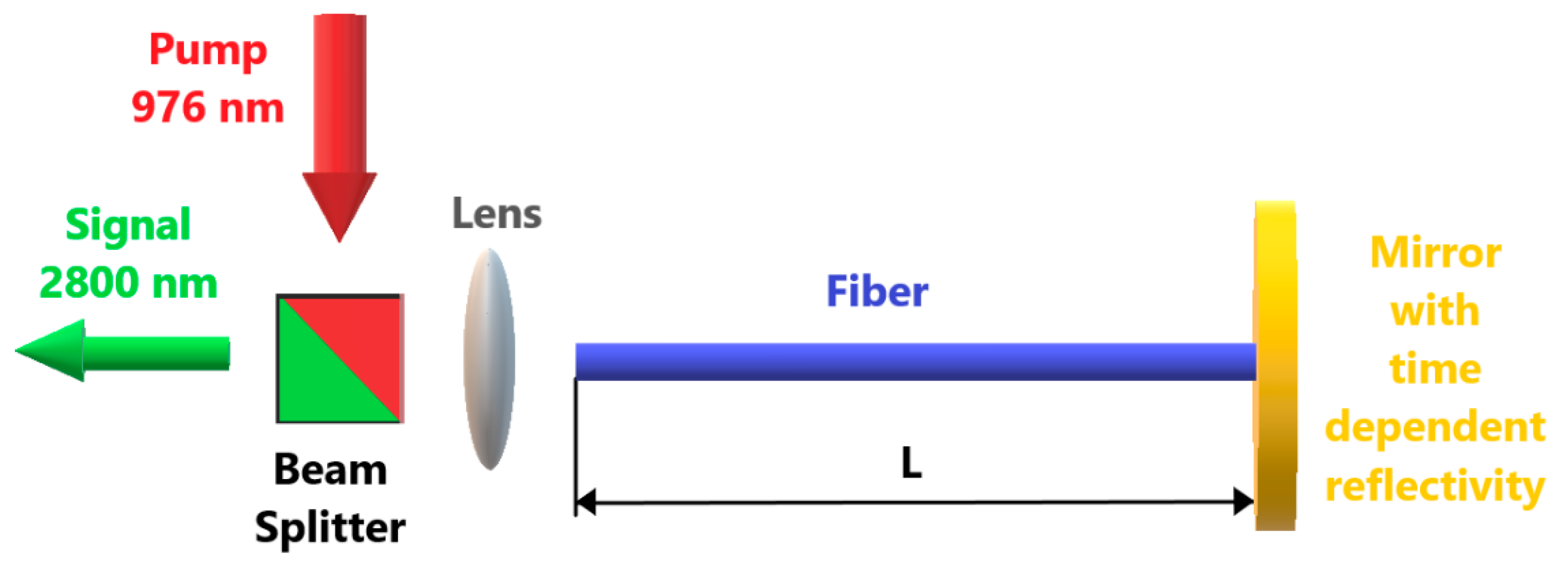
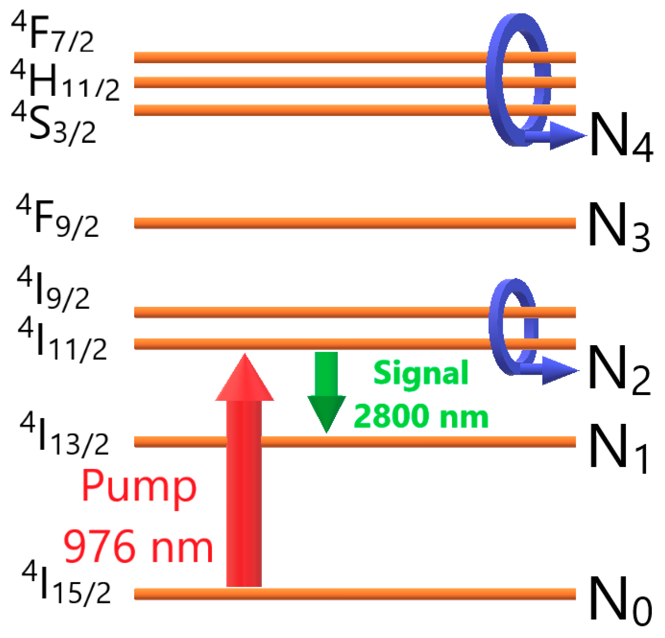
Figure 1 shows a schematic diagram of a Q-switched fiber laser cavity, which is the subject of the numerical investigation. The action of the Q-switch is approximated by a mirror with a time dependent reflectivity positioned at z = L. The pump light is delivered to the fiber at z = 0 using a beam splitter, which also allows extraction of the infrared signal at the same end of the fiber. The fiber used is made of fluoride glass doped with trivalent erbium ions. The energy level diagram for trivalent erbium ion is shown in Figure 2. The pumping wavelength is 976 nm, whilst the infrared signal is at a wavelength of 2800 nm. Levels 4F7/2, 4H11/2 and 4S3/2 are thermally coupled, and represented in the model as one level N4. Similarly, thermal coupling occurs for N2, which represents coupled levels 4I9/2 and 4I11/2. The higher lying levels, i.e., N3 and N4, are populated by an up-conversion processes. The temporal dependence of energy level populations for the energy level system shown in Figure 2 can be calculated by solving a set of differential equations, which can be derived using a rate equations approach [17]:
The energy level populations fulfill the condition N0 + N1 + N2 + N3 + N4 = N. The ground state absorption rate RGSA and the stimulated emission rate RSE are given by [21]:
The power distributions for forward (denoted with upper index ‘+’) and backward (denoted with upper index ‘−’) propagating pump and signal waves, denoted in (2) respectively as Pp and Ps, are obtained by solving a set of partial differential equations:
The partial differential Equations (1) and (3) are coupled together, and hence have to be solved simultaneously. Additionally, for the laser cavity configuration shown in Figure 1, the following boundary conditions apply at z = 0 and z = L:
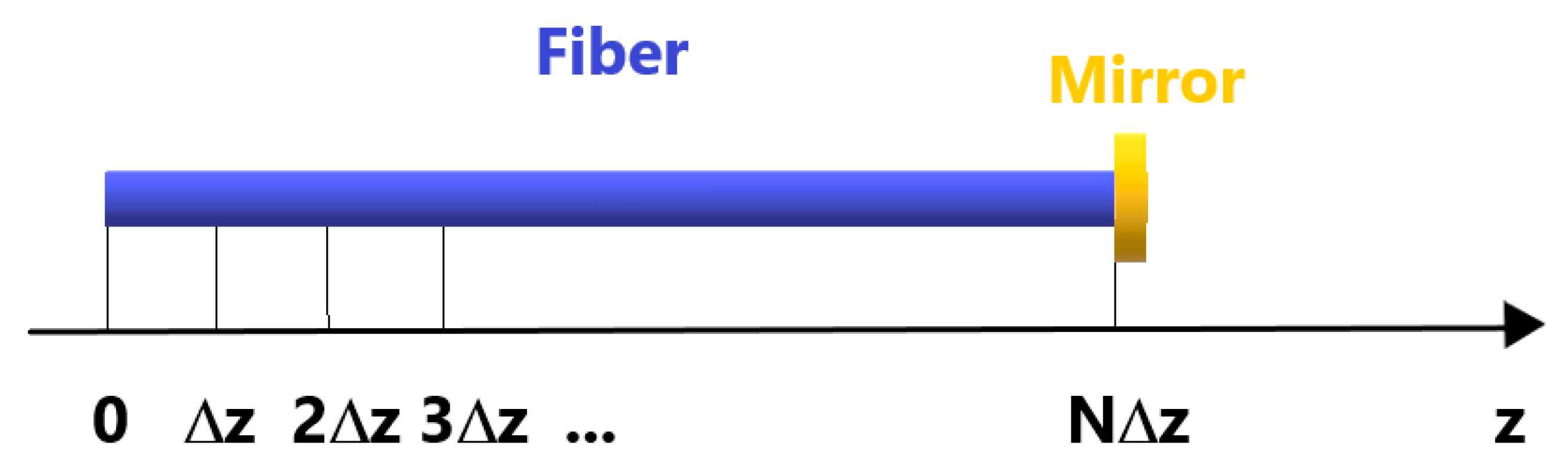
At a set of sampling points, z = zi selected along the z axis (Figure 3) partial differential Equations (1) and (3) can be reduced to a set of ordinary differential Equations (5) and (6):
where the finite difference operator , which approximates the spatial derivative of pump and signal power with respect to z is:
for all sampling points except those which are adjacent to the fiber facets. The finite difference approximations near facets are obtained using the extended Taylor series following the formalism presented in detail in [18]. The finite difference approximation (7) is second order accurate. In, principle, other finite difference approximation orders could be used in (6); however, the results presented in [18] show that the second order approximation gives a significant advantage over the first order one, whilst remaining simple to implement.
The numerical integration of Equations (5) and (6) has to be carried out using an algorithm designated for handling stiff differential equations.
The flowchart showing the steps leading to a calculation of an output pulse shape generated by a Q-switched fiber laser is illustrated in Figure 4. The numerical calculations are initiated from an arbitrary initial guess fed to a steady state solver, which calculates a self-consistent solution of Equations (1) and (3) for ∂/∂t = 0. The steady state solution is obtained using a relaxation method. Subsequently the steady state solution is refined using the time domain model. This step helps in avoiding numerical artefacts, which could result from a mismatch between a numerical solution calculated by the relaxation method, and the one obtained using the time domain method. Such a mismatch can be particularly large at low spatial finite difference mesh resolutions in the time domain model. In the last step, a time domain analysis of the Q-switched fiber laser pulses is performed.
In the next section we apply the numerical model following an algorithm, which is depicted by the flowchart shown in Figure 4, and discuss the results obtained.
3. Results and Discussion
The values of the numerical parameters are summarized in Table 1, and are applied throughout this section unless otherwise stated. The values of the branching rations and energy level lifetimes are given in Table 2 [21]. The spontaneous emission parameter γsp has been approximated using an equation derived in [22]:
where ν is the signal frequency corresponding to the wavelength of 2800 nm, while Δν is assumed to be equal to 10 nm, following the experimental results presented in [9].
First, a study of the steady state characteristics of the fiber laser is performed. Figure 5. shows the dependence of the output signal power on the pump power for a 2 m long fiber with 0.04 reflectivity for signal wave at z = L. Both linear and logarithmic scales are used to present the results, in order to show in more detail the behavior of the fiber laser near threshold. The lasing threshold occurs near 1.8 W of pumping power. When the facet reflectivity for signal wave at z = L is increased to 0.2, the threshold pump power decreases significantly to nearly 1.3 W (Figure 6). Further, the laser differential and wall-plug efficiency increase.
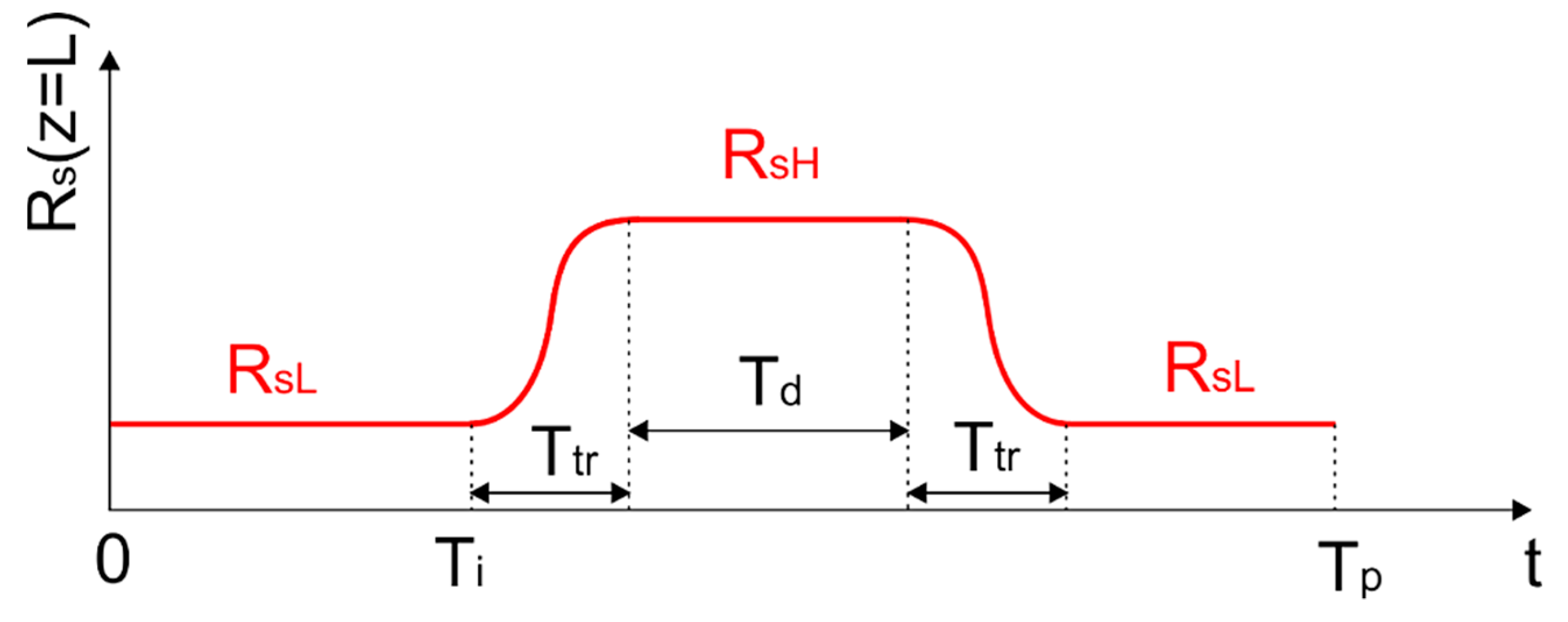
After discussing the static characteristics of the fiber laser, the discussion moves to the time domain analysis of the Q-switched pulses. Figure 7 shows the time dependence of the facet reflectivity on time, as used in the time domain simulations of the Q-switched laser operation. In the following simulations, the RsL is equal to 0.04, while RsH is equal to 0.2. Therefore, the laser cavity is effectively switched between the two steady states considered in simulation results presented in Figure 5 and Figure 6. The value of the initial leading time Ti is assumed to be equal to zero. The time of the signal duration Td is equal to 1 µs, while the time of the entire period Tp is equal to 30 ms. The transition time Ttr is equal to 200 ns, unless otherwise stated. During the transition, the pulse follows the sine squared (rising edge) or cosine squared (descending edge) shape considered within the first quadrant.
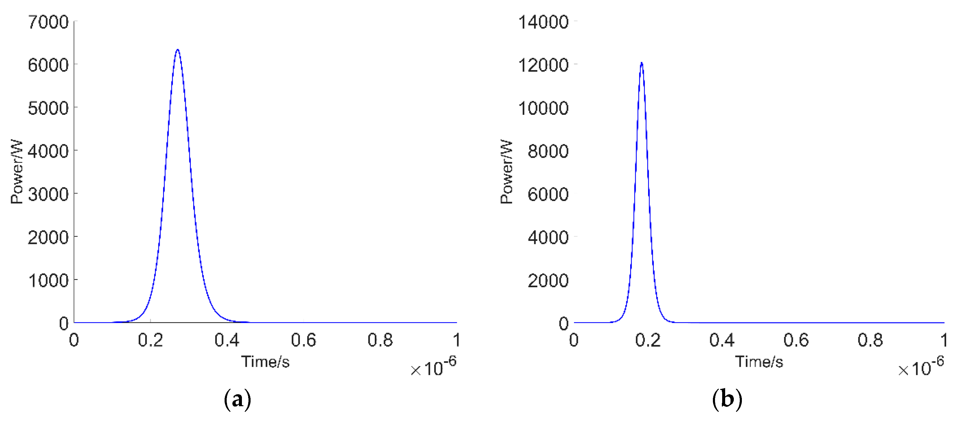
Figure 8 shows a numerically calculated dependence of the output power on time for a 2 m long fiber with the facet reflectivity for signal wave at z = L switched between 0.04 and 0.2, at four selected values of the pump power: 1.2 W (a), 1.5 W (b), 2 W (c) and 8 W (d). The pump powers were selected to study a Q-switched laser operation in four different situations. Only the first microsecond is presented to show the shape of the generated pulse. At a pump power of 1.2 W, the fiber laser operates in a steady state below the threshold for the value of the facet reflectivity of both 0.04 and 0.2. At 1.5 W, the fiber laser operates below the threshold, with a facet reflectivity equal to 0.04 only, while at 0.2 it operates above the threshold. When the pump power equals 2 W, the fiber laser operates just above the threshold, both before and after switching. When the pump power is further raised to 8 W, one investigates the fiber laser’s operation during Q-switching well above the lasing threshold. The results presented in Figure 8a show that when the laser operates below threshold, a low intensity pulse is formed. The pulse shape does not follow the switching pulse shape shown in Figure 7 exactly. The signal power increases approximately seven fold, while the facet reflectivity increases only five fold. When the pump power is increased to a value larger than the lasing threshold pump power for facet reflectivity, 0.04 (Figure 8b), a pulse is generated with a shape typical for Q-switching. The pulse has a fairly large delay when compared to the switching pulse raising edge (Figure 7). The delay results from the time needed to build up the pulse power within the cavity during subsequent round-trips after the raising edge of the facet reflectivity switching pulse. When the pump power is sufficient to reach the lasing threshold both before and after switching (Figure 8c), the pulse becomes narrower, and the delay of the pulse significantly reduces when compared to that presented in Figure 8b. Also, one can observe that pulse width narrowing is accompanied by a significant increase in the peak pulse power, from approximately 2.5 kW to nearly 10 kW. It is also noted that such output pulse peak power levels are observed in experiments. Further increasing of the pump power has only a negligible effect on the generated pulse shape (Figure 8d). There is only a small temporal shift of the pulse. This suggests that larger pump power allows for faster power build up within the cavity, which agrees with an intuitive guess. Finally, it is noted that with γsp in Equation (2) equal to zero, it is not possible to numerically model the pulse behavior below the lasing threshold, since a model without a spontaneous emission term would yield zero output power value. Thus, inclusion of spontaneous emission is essential in these simulations. The importance of the spontaneous emission will be further explored when discussing the behavior of the Q-switched laser cavity generating pulse trains.
Figure 9 shows a numerically calculated dependence of the energy level populations on time for a 2 m long fiber, with the facet reflectivity for signal wave at z = L switched between 0.04 and 0.2. Four selected values of the pump power are considered: 1.2 W (a), 1.5 W (b), 2 W (c) and 8 W (d). The results from Figure 9 show that below the lasing threshold (Figure 9a), the generated pulse has practically no impact on the level populations due to its low photon density. However, above the lasing threshold, the pulse photon density achieves large values, and significantly depletes the population of level 2 (Figure 9b), which is accompanied by an increase of the level 1 population. The recovery to the steady state after the depletion is very slow, taking more than 1 ms. This slow recovery process can be sped up by increasing the pump power, as can be observed by comparing the results shown in Figure 9b,d. The effect of photon density reduction accompanied by slow recovery of the energy level populations puts a limit on the maximum repetition rate of a stable pulse train generated by a Q-switched laser. Namely, before the next pulse can be generated, the photon density of the signal wave has to return nearly to the steady state equilibrium. Otherwise, there is no guarantee that the generated pulse train will be stable and have no jitter. A value of the photon intensity before the onset of the switching pulse, which is significantly lower than in the steady state, would translate into a longer time needed to build up the signal power within the cavity, and hence, could result in a larger pulse delay for the second pulse than for the first.
Figure 10 shows numerically calculated dependence of the pulse output power on time for a 2 m long fiber, with the facet reflectivity for signal wave at z = L switched between 0.04 and 0.2 at four selected values of the transition time Ttr: 100 ns (a), 50 ns (b), 400 ns (c) and 600 ns (d). The pump power used in these simulations was 8 W. One can observe that reducing the transition time below 200 ns has no significant impact on the pulse appearance. The only effect observed is a small change of the pulse position. It is interesting to note that the 200 ns switching time is sufficient to obtain optimal performance in a cavity with round trip time of approximately 40 ns, and 5 fold change of the facet reflectivity during switching. A significant reduction of the peak pulse power occurs, however, when the transition time is increased to 400 ns; a further reduction of the peak pulse power takes place by increasing the transition time to 600 ns. However, we note that even with a 600 ns switching pulse transition time, a high peak power, and a fairly narrow Q-switched pulse, can still be generated.
In Figure 11, a study of the impact of the fiber length on the pulse shape is performed. These results show that the fiber length has a major impact on both the pulse width and pulse peak power. By reducing the fiber length, one reduces the pulse round trip time, and thus allows for a faster buildup of power within the fiber laser cavity. This results in the generation of shorter pulses, which is also accompanied by a higher value of the peak power. Thus, one has to be cautious when reducing the fiber length whilst trying to reduce the pulse duration, because the peak power increases concurrently, and high photon density within the fiber laser cavity may damage the fiber.
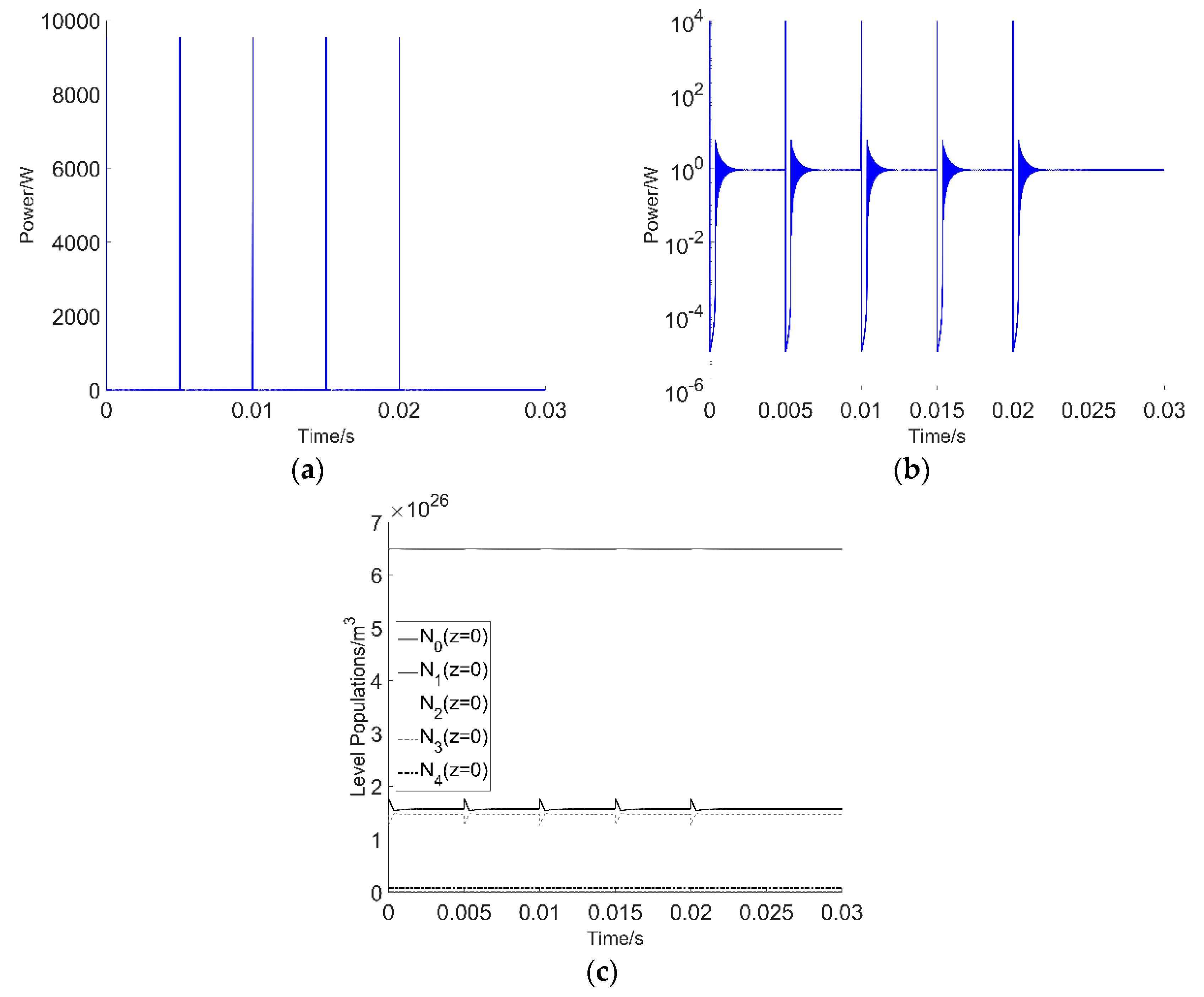
Finally, a numerical simulation is performed for calculation of a train of 5 Q-switched pulses. These results demonstrate the importance of the spontaneous emission, even if the fiber laser operates above the threshold before and after switching. Figure 12 shows a numerically calculated dependence of the output power and energy level populations on time for 5 pulses at Ttr = 200 ns, with the facet reflectivity for signal wave at z = L switched between 0.04 and 0.2, L = 2 m, and a pump power of 8 W. These results were obtained by repeating the waveform from Figure 7 five times, with Tp = 5 ms. The results from Figure 12a show a stable train of five pulses, calculated by the numerical algorithm. Figure 5b shows the same result as Figure 5a, but with the vertical axis scaled logarithmically. Such scaling is needed to show the effect of photon population depletion, which follows the Q-switched pulse. This results from the fact that the level 2 population is drained by the Q-switched pulse. This in turn results in a very low value of signal gain, and a subsequent reduction of the photon population within the laser cavity. As shown in Figure 12b,c the recovery process and a return to a steady state equilibrium is slow.
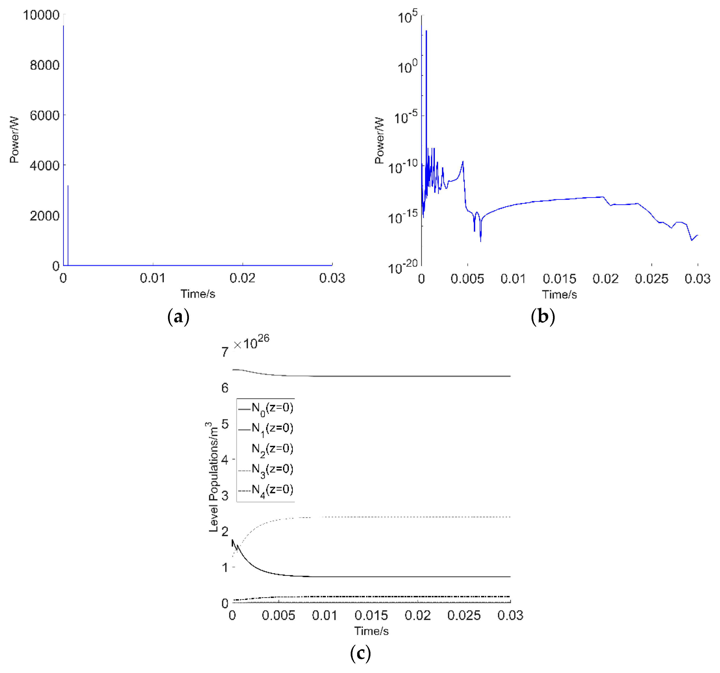
In Figure 13, the results are shown of an attempt to recalculate the results shown in Figure 12 without including the effect of the spontaneous emission, i.e., by setting γsp in Equation (1) to zero. Only the first pulse could be reproduced accurately. The model that does not include spontaneous emission could not correctly reproduce the process of photon population build up and energy level population recovery to the steady state equilibrium. This demonstrates that the spontaneous emission process plays an essential role in these simulations. This is because after the pulse trailing edge, the photon population drops to a very low level. At low photon densities, the spontaneous emission contribution to the growth of the photon population within the cavity dominates, and is more significant than the photon population growth resulting from the optical gain. Hence, the calculated time dependence for signal power and of the level populations differ significantly from those presented in Figure 12.
4. Conclusions
In summary, a comprehensive model for analyzing the Q-switched operation of a fluoride fiber laser doped with erbium ions is presented. An analysis of the pulse shape dependence on the pump power, fiber length, and switching time is given. The results obtained show that an inclusion of the spontaneous emission process for the signal wave in the fiber laser model is essential when calculating numerically the output pulse shape, especially when analyzing the process of pulse train generation.
Acknowledgments
The author wishes to thank Wrocław University of Science and Technology (statutory activity) for financial support.
Conflicts of Interest
The author declares no conflict of interest.
References
- Schneider, J.; Carbonnier, C.; Unrau, U.B. Characterization of a Ho3+-doped fluoride fiber laser with a 3.9-μm emission wavelength. Appl. Opt. 1997, 36, 8595–8600. [Google Scholar] [CrossRef] [PubMed]
- Qin, Z.P.; Xie, G.Q.; Ma, J.G.; Yuan, P.; Qian, L.J. Mid-infrared Er: ZBLAN fiber laser reaching 3.68 μm wavelength. Chin. Opt. Lett. 2017, 15, 111402. [Google Scholar]
- Henderson-Sapir, O.; Munch, J.; Ottaway, D.J. Mid-infrared fiber lasers at and beyond 3.5 μm using dual-wavelength pumping. Opt. Lett. 2014, 39, 493–496. [Google Scholar] [CrossRef] [PubMed]
- Tokita, S.; Murakami, M.; Shimizu, S.; Hashida, M.; Sakabe, S. Liquid-cooled 24 W mid-infrared Er: ZBLAN fiber laser. Opt. Lett. 2009, 34, 3062–3064. [Google Scholar] [CrossRef] [PubMed]
- Faucher, D.; Bernier, M.; Androz, G.; Caron, N.; Vallee, R. 20 W passively cooled single-mode all-fiber laser at 2.8 μm. Opt. Lett. 2011, 36, 1104–1106. [Google Scholar] [CrossRef] [PubMed]
- Woodward, R.; Majewski, M.; Bharathan, G.; Hudson, D.; Fuerbach, A.; Jackson, S. Watt-level dysprosium fiber laser at 3.15 μm with 73% slope efficiency. Opt. Lett. 2018, 43, 1471–1474. [Google Scholar] [CrossRef] [PubMed]
- Majewski, M.R.; Woodward, R.I.; Carreé, J.-Y.; Poulain, S.; Poulain, M.; Jackson, S.D. Emission beyond 4 μm and mid-infrared lasing in a dysprosium-doped indium fluoride (InF 3) fiber. Opt. Lett. 2018, 43, 1926–1929. [Google Scholar] [CrossRef] [PubMed]
- Tokita, S.; Murakami, M.; Shimizu, S.; Hashida, M.; Sakabe, S. 12 WQ-switched Er: ZBLAN fiber laser at 2.8 μm. Opt. Lett. 2011, 36, 2812–2814. [Google Scholar] [CrossRef] [PubMed]
- Lamrini, S.; Scholle, K.; Schäfer, M.; Ward, J.; Francis, M.; Farries, M.; Sujecki, S.; Benson, T.; Seddon, A.; Oladeji, A.; et al. High-Energy Q-switched Er: ZBLAN Fibre Laser at 2.79 μm. In Proceedings of the 2015 European Conference on Lasers and Electro-Optics, Munich, Germany, 21–25 June 2015. [Google Scholar]
- Jobin, F.; Fortin, V.; Maes, F.; Bernier, M.; Vallée, R. Gain-switched fiber laser at 3.55 µm. Opt. Lett. 2018, 43, 1770–1773. [Google Scholar] [CrossRef] [PubMed]
- Gorjan, M.; Marincek, M.; Copic, M. Pump absorption and temperature distribution in erbium-doped double-clad fluoride-glass fibers. Opt. Express 2009, 17, 19814–19822. [Google Scholar] [CrossRef] [PubMed]
- Gorjan, M.; Marincek, M.; Copic, M. Spectral dynamics of pulsed diode-pumped erbium-doped fluoride fiber lasers. J. Opt. Soc. Am. B 2010, 27, 2784–2793. [Google Scholar] [CrossRef]
- Gorjan, M.; Marincek, M.; Copic, M. Role of Interionic Processes in the Efficiency and Operation of Erbium-Doped Fluoride Fiber Lasers. IEEE J. Quantum Electr. 2011, 47, 262–273. [Google Scholar] [CrossRef]
- Jackson, S.D.; Pollnau, M.; Li, J. Diode Pumped Erbium Cascade Fiber Lasers. IEEE J. Quantum Electr. 2011, 47, 471–478. [Google Scholar] [CrossRef]
- Li, J.; Gomes, L.; Jackson, S.D. Numerical Modeling of Holmium-Doped Fluoride Fiber Lasers. IEEE J. Quantum Electr. 2012, 48, 596–607. [Google Scholar] [CrossRef]
- Li, J.; Luo, H.; Liu, Y.; Zhang, L.; Jackson, S.D. Modeling and Optimization of Cascaded Erbium and Holmium Doped Fluoride Fiber Lasers. IEEE J. Sel. Top. Quantum Electr. 2014, 20, 0900414. [Google Scholar]
- Zhu, G.; Zhu, X.; Norwood, R.A.; Peyghambarian, N. Experimental and Numerical Investigations on Q-Switched Laser-Seeded Fiber MOPA at 2.8 μm. J. Lightw. Technol. 2014, 32, 3951–3955. [Google Scholar] [CrossRef]
- Sujecki, S. Simple and efficient method of lines based algorithm for modeling of erbium doped Q-switched fluoride fiber lasers. J. Opt. Soc. Am. B 2016, 33, 2288–2295. [Google Scholar] [CrossRef]
- Sujecki, S. Arbitrary truncation order three-point finite difference method for optical waveguides with stepwise refractive index discontinuities. Opt. Lett. 2010, 35, 4115–4117. [Google Scholar] [CrossRef] [PubMed]
- Sujecki, S. Extended Taylor series and interpolation of physically meaningful functions. Opt. Quantum Electr. 2013, 45, 53–66. [Google Scholar] [CrossRef]
- Li, J.; Jackson, S.D. Numerical Modeling and Optimization of Diode Pumped Heavily-Erbium-Doped Fluoride Fiber Lasers. IEEE J. Quantum Electr. 2012, 48, 454–464. [Google Scholar] [CrossRef]
- Becker, P.M.; Olsson, A.A.; Simpson, J.R. Erbium Doped Amplifiers. Fundamentals and Technology; Academic Press: London, UK, 1999. [Google Scholar]
Figure 1.
Schematic diagram of the Q-switched fiber laser cavity.

Figure 2.
Energy level diagram for a trivalent erbium ion.

Figure 3.
Schematic diagram illustrating the finite difference discretization.

Figure 4.
Flowchart showing the sequence followed during numerical calculations.
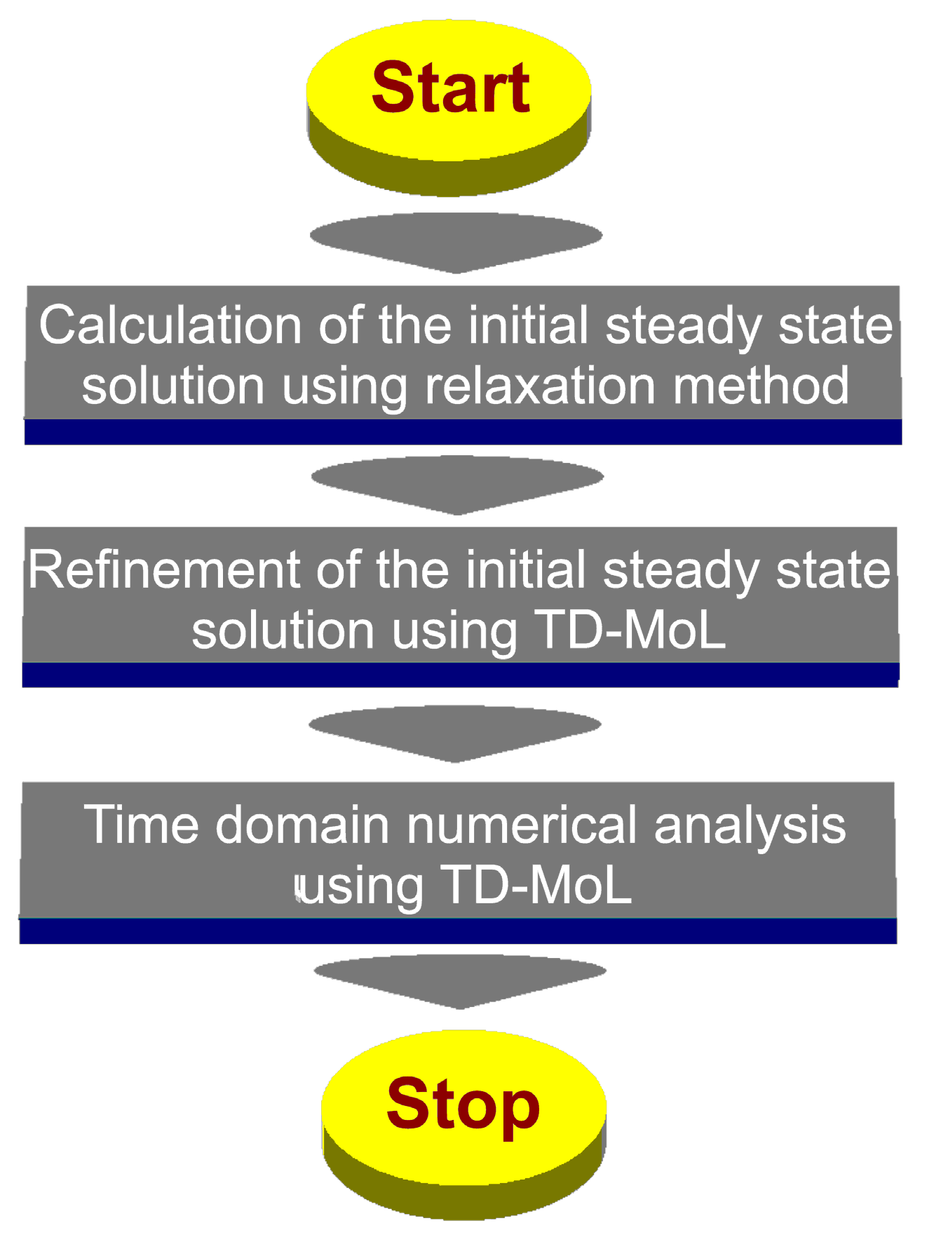
Figure 5.
Numerically calculated dependence of the output signal power on the pump power for a 2 m fiber length and 0.04 reflectivity for signal at z = L: (a) Presented on a linear scale. The inset shows zoomed region near the lasing threshold; (b) Presented on a logarithmic scale.
Figure 5.
Numerically calculated dependence of the output signal power on the pump power for a 2 m fiber length and 0.04 reflectivity for signal at z = L: (a) Presented on a linear scale. The inset shows zoomed region near the lasing threshold; (b) Presented on a logarithmic scale.

Figure 6.
Numerically calculated dependence of the output signal power on the pump power for a 2 m fiber length and 0.2 reflectivity for signal at z = L: (a) Presented on a linear scale. The inset shows zoomed region near the lasing threshold; (b) Presented on a logarithmic scale.
Figure 6.
Numerically calculated dependence of the output signal power on the pump power for a 2 m fiber length and 0.2 reflectivity for signal at z = L: (a) Presented on a linear scale. The inset shows zoomed region near the lasing threshold; (b) Presented on a logarithmic scale.
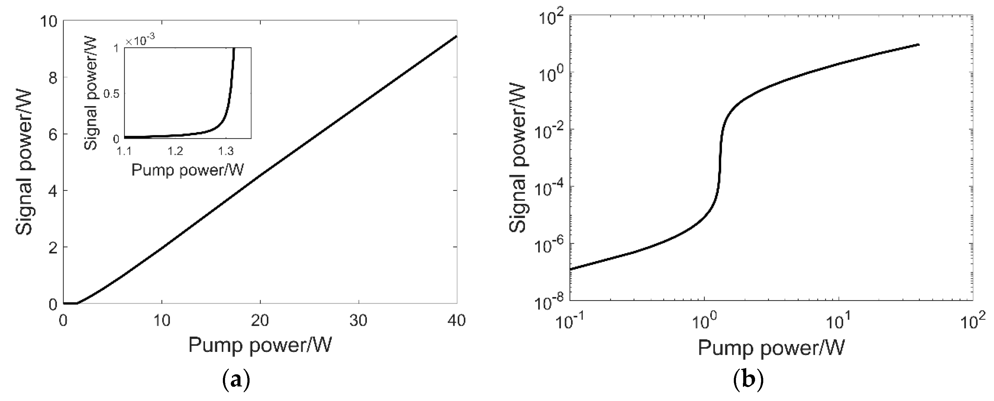
Figure 7.
The time dependence of facet reflectivity at z = L for signal wave.

Figure 8.
Numerically calculated dependence of the output power on time for a 2 (m) long fiber with the facet reflectivity for signal wave at z = L switched between 0.04 and 0.2 and Ttr = 200 (ns): (a) At pump power of 1.2 (W); (b) At pump power of 1.5 (W); (c) At pump power of 2 (W); (d) At pump power of 8 (W).
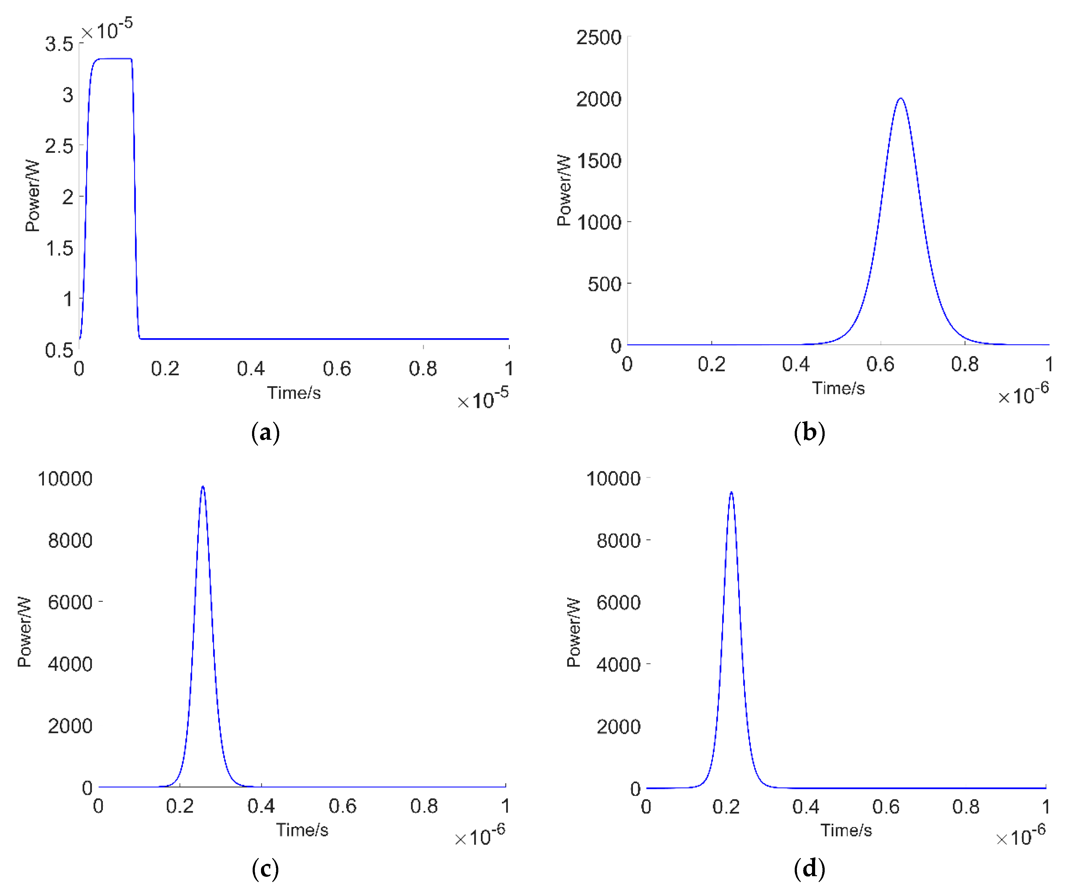
Figure 9.
Numerically calculated dependence of the energy level populations on time for a 2 (m) long fiber with the facet reflectivity for signal wave at z = L switched between 0.04 and 0.2 and 0.2 and Ttr = 200 (ns): (a) At pump power of 1.2 (W); (b) At pump power of 1.5 (W); (c) At pump power of 2 (W); (d) At pump power of 8 (W).
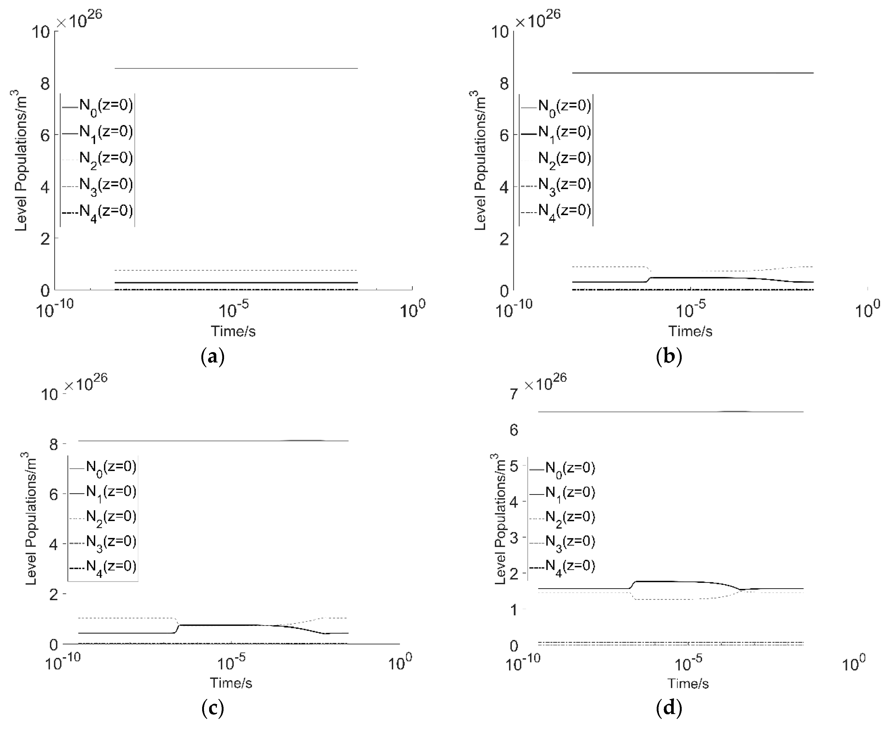
Figure 10.
Numerically calculated dependence of the output power on time for a 2 (m) long fiber with the facet reflectivity for signal wave at z = L switched between 0.04 and 0.2 and pump power of 8 (W): (a) For Ttr = 100 (ns); (b) For Ttr = 50 (ns); (c) For Ttr = 400 (ns); (d) For Ttr = 600 (ns).
Figure 10.
Numerically calculated dependence of the output power on time for a 2 (m) long fiber with the facet reflectivity for signal wave at z = L switched between 0.04 and 0.2 and pump power of 8 (W): (a) For Ttr = 100 (ns); (b) For Ttr = 50 (ns); (c) For Ttr = 400 (ns); (d) For Ttr = 600 (ns).
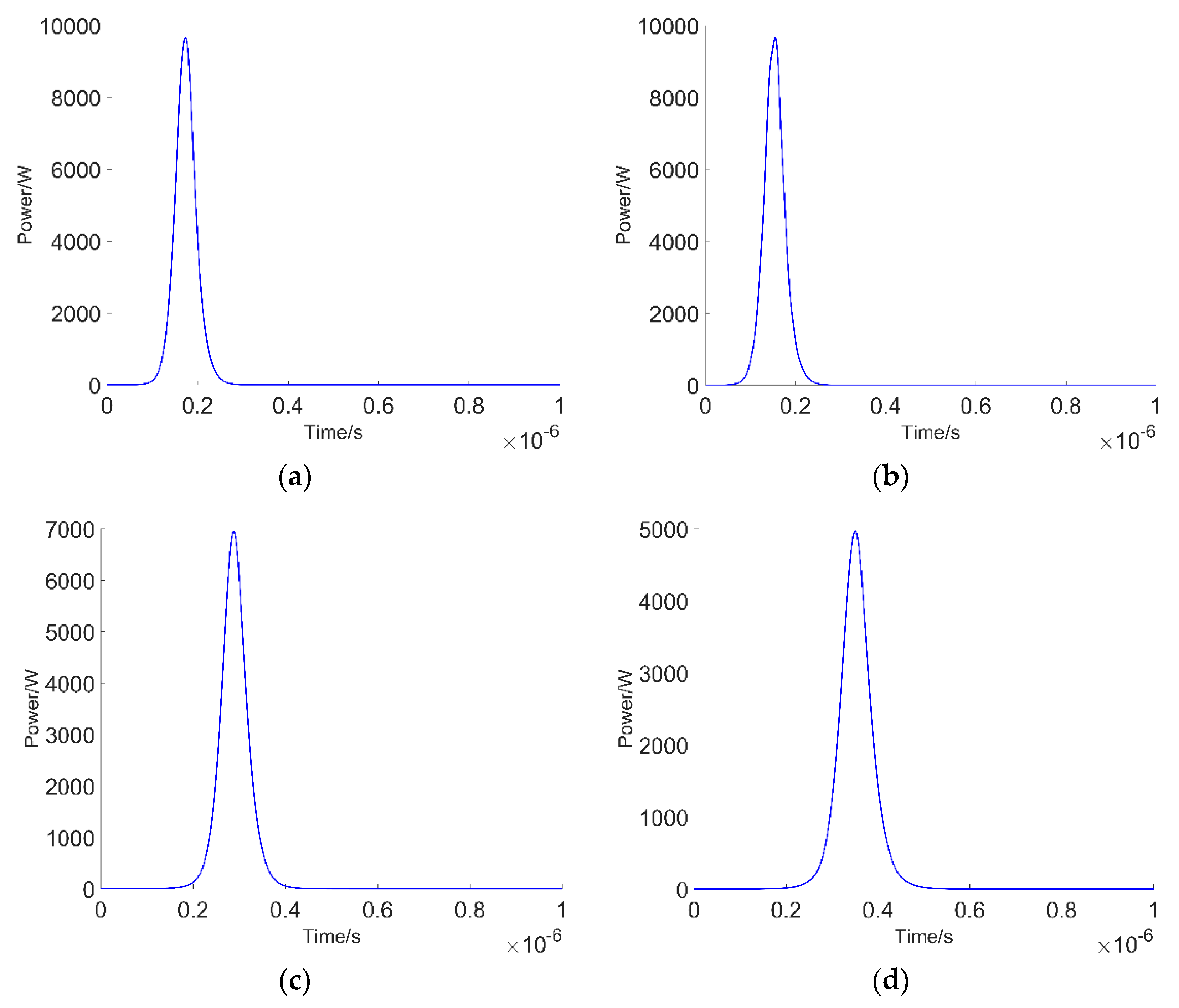
Figure 11.
Numerically calculated dependence of the output power on time at Ttr = 200 (ns) with the facet reflectivity for signal wave at z = L switched between 0.04 and 0.2 and pump power of 8 (W): (a) For L = 3 (m); (b) For L = 1.5 (m).
Figure 11.
Numerically calculated dependence of the output power on time at Ttr = 200 (ns) with the facet reflectivity for signal wave at z = L switched between 0.04 and 0.2 and pump power of 8 (W): (a) For L = 3 (m); (b) For L = 1.5 (m).

Figure 12.
Numerically calculated dependence of the output power and energy level populations on time for 5 pulses at Ttr = 200 (ns) with the facet reflectivity for signal wave at z = L switched between 0.04 and 0.2, L = 2 (m) and pump power of 8 (W): (a) Output power on linear scale; (b) Output power with vertical logarithmic scale; (c) energy level populations.

Figure 13.
Numerically calculated dependence of the output power and energy level populations on time for 5 pulses at Ttr = 200 (ns) with the facet reflectivity for signal wave at z = L switched between 0.04 and 0.2, L = 2 (m) and pump power of 8 (W): (a) Output power on linear scale; (b) Output power with vertical logarithmic scale; (c) energy level populations. In these simulations the spontaneous emission coefficient γsp (Equation (1)) was assumed equal to zero.


Table 1.
Modelling parameters.
| Parameter | Unit | Value |
|---|---|---|
| b1/b2 | 0.1/0.16 | |
| W11 | m3/s | 1 × 10⁻²⁴ |
| W22 | m3/s | 0.3 × 10⁻²⁴ |
| λp | m | 976 × 10−9 |
| λs | m | 2.8 × 10⁻⁶ |
| σGSA | m2 | 2.1 × 10⁻²⁵ |
| σSE | m2 | 4.5 × 10⁻²⁵ |
| NEr | 1/m3 | 9.6 × 1026 |
| L | m | 2 |
| Гp | 0.011 | |
| Гs | 1.0 | |
| αp | 1/m | 23 × 10−3 |
| αs | 1/m | 3.0 × 10⁻³ |
| Rp(z = 0) | 0 | |
| Rp(z = L) | 0.04 | |
| Rs(z = 0) | 0.04 | |
| Rs(z = L) | 0.04 |
Table 2.
Branching ratios and level lifetimes.
| Parameter | Unit | Value |
|---|---|---|
| τ1 | ms | 9 |
| τ2 | ms | 6.9 |
| τ3 | ms | 0.12 |
| τ4 | ms | 0.57 |
| β21, β20 | 0.37, 0.63 | |
| β32, β31,β30 | 0.856, 0.004, 0.014 | |
| β43, β42, β41, β40 | 0.34, 0.04, 0.18, 0.44 |
© 2018 by the author. Licensee MDPI, Basel, Switzerland. This article is an open access article distributed under the terms and conditions of the Creative Commons Attribution (CC BY) license (http://creativecommons.org/licenses/by/4.0/).
Share and Cite
MDPI and ACS Style
Sujecki, S. Numerical Analysis of Q-Switched Erbium Ion Doped Fluoride Glass Fiber Laser Operation Including Spontaneous Emission. Appl. Sci. 2018, 8, 803. https://doi.org/10.3390/app8050803
AMA Style
Sujecki S. Numerical Analysis of Q-Switched Erbium Ion Doped Fluoride Glass Fiber Laser Operation Including Spontaneous Emission. Applied Sciences. 2018; 8(5):803. https://doi.org/10.3390/app8050803
Chicago/Turabian StyleSujecki, Sławomir. 2018. "Numerical Analysis of Q-Switched Erbium Ion Doped Fluoride Glass Fiber Laser Operation Including Spontaneous Emission" Applied Sciences 8, no. 5: 803. https://doi.org/10.3390/app8050803
Note that from the first issue of 2016, this journal uses article numbers instead of page numbers. See further details here.