Determination of Geometrical REVs Based on Volumetric Fracture Intensity and Statistical Tests


Abstract
:1. Introduction
2. The Establishment of a 3D Fracture Network Model
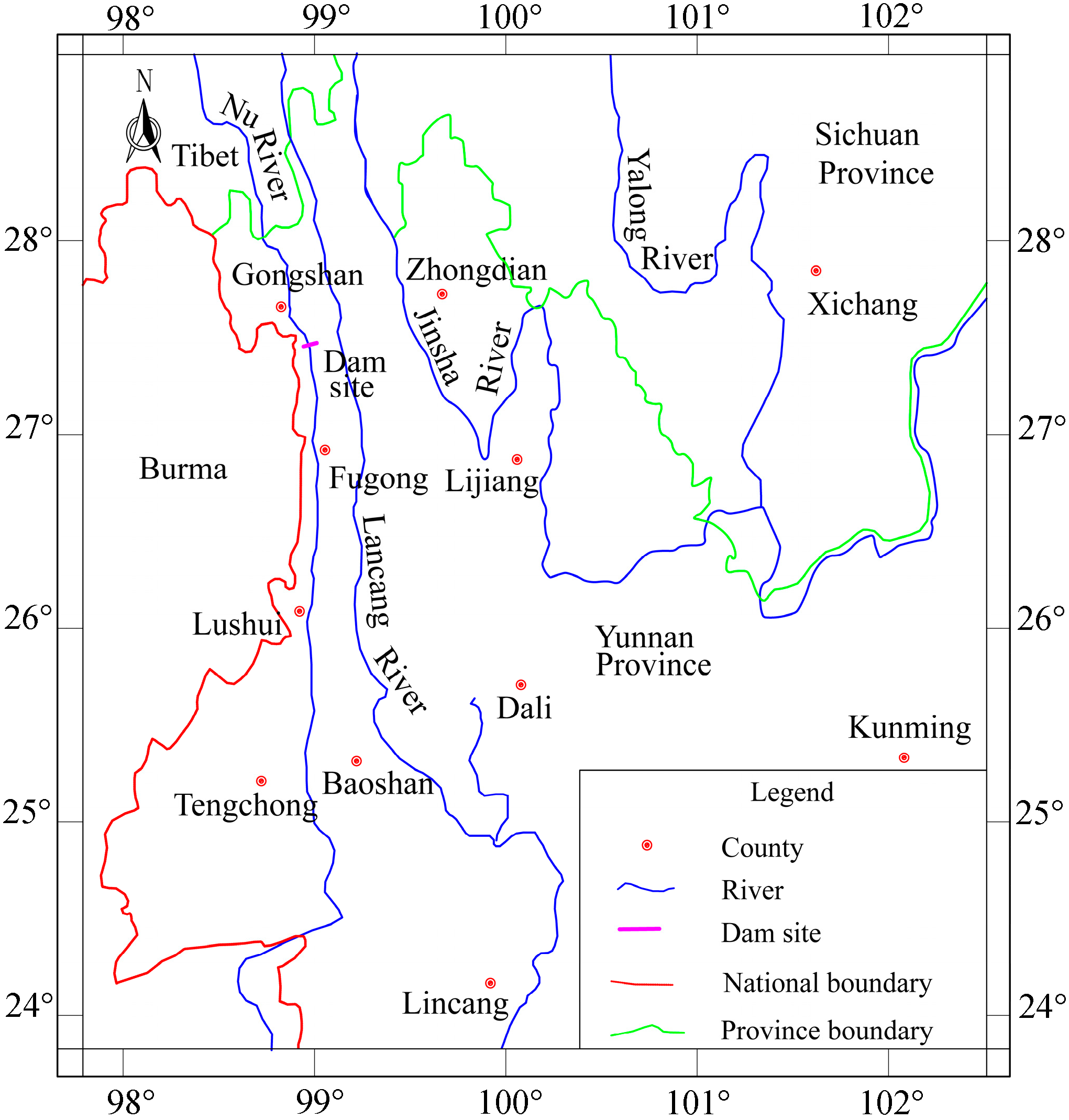
2.1. Data Collection from the Study Area
2.2. 3D Fracture Network Modeling
- The discontinuities are thin planar discs with a random distribution.
- The fractures are not open; water and fracture fill can be disregarded.
3. Methodology
3.1. Likelihood Ratio Test
3.2. Wald–Wolfowitz Runs Test
- The merged samples X and Y are sorted in ascending order, and sample X is coded as a “1”, while sample Y is coded as a “2”.
- Each observation is replaced by a label, “1” or “2”, depending upon the sample to which it originally belonged.
- Calculate the number (run) of a consecutive sequence of identical labels (“1” or “2”).
- To determine the test statistic, when both m and n are less than or equal to 20, the test statistic is the total number of runs, U. The critical value U is obtained from the table of the Wald–Wolfowitz runs test. When the number of observations is larger than 20, U follows a normal distribution asymptotically. The expected number of runs and variance are given as
- The value is calculated based on the small U value or the test statistic Z obtained from the normal distribution. In this study, the REV size of a rock mass was determined based on the statistical similarity between two compared samples. When the significance level values exceed a threshold level of 0.05, the fluctuation in P32 values significantly decreases as the sample size increases, and the P32 values of two compared samples are considered statistically similar. To better demonstrate the procedure of detecting the REV size by using these two statistical test methods, a calculation flow chart is provided in Figure 5.
4. Determination of the Geometrical REV
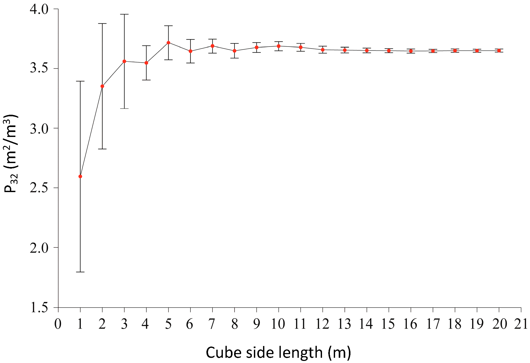
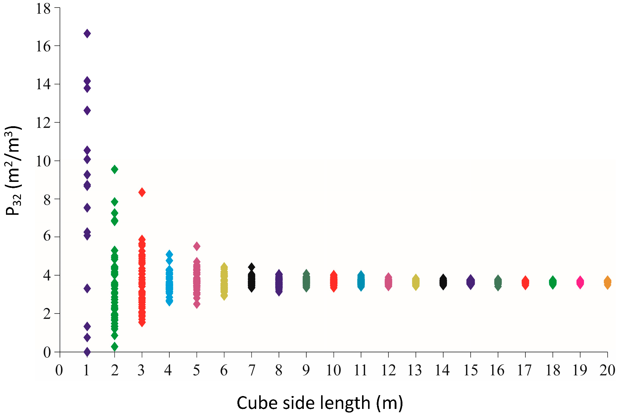
4.1. P32 Characteristics
4.2. REV Size Based on Statistical Tests
5. Discussion
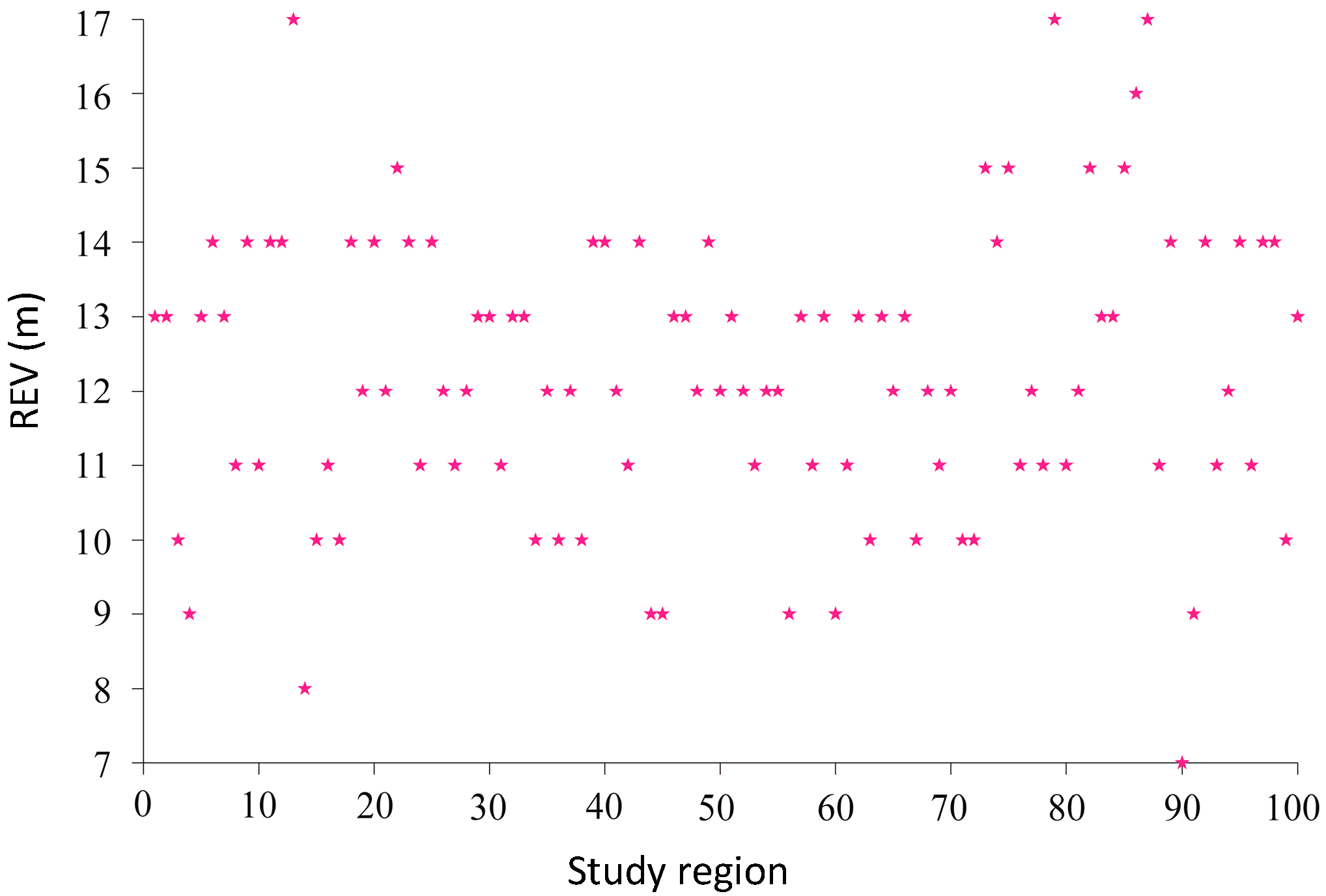
5.1. Investigation of the REV Size
5.2. Geometrical REV Calculation
- Generate a reliable 3D fracture network model based on the joint data obtained from the field survey.
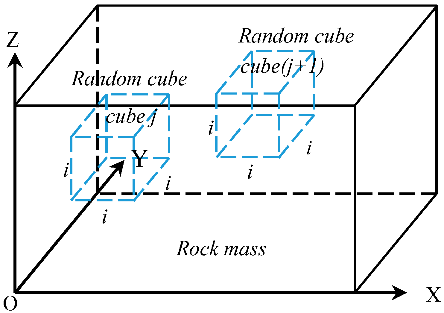
- Select several random regions in the generated 3D fracture network model.
- Calculate the geometrical parameters of fractured rock masses by varying cube sizes and locations. Generally, the fracture intensity index is widely applied.
- Generate n samples with the same cube size, which vary from 1 to n m.
- Analyze the REV size by using several different statistical test methods.
6. Conclusions
Author Contributions
Acknowledgments
Conflicts of Interest
References
- Song, S.Y.; Sun, F.Y.; Chen, J.P.; Zhang, W.; Han, X.D.; Zhang, X.D. Determination of RVE size based on the 3D fracture persistence. Q. J. Eng. Geol. Hydrogeol. 2017, 50, 60–68. [Google Scholar] [CrossRef]
- Bear, J. Dynamics of Fluids in Porous Media; American Elsevier: New York, NY, USA, 1972. [Google Scholar]
- Long, J.C.S.; Remer, J.S.; Wilson, C.R.; Witherspoon, P.A. Porous media equivalents for networks of discontinuous fractures. Water Resour. Res. 1982, 18, 645–658. [Google Scholar] [CrossRef]
- Kulatilake, P.H.S.W.; Panda, B.B. Effect of block size and joint geometry on jointed rock hydraulics and REV. J. Eng. Mech. 2000, 126, 850–858. [Google Scholar] [CrossRef]
- Wang, M.; Kulatilake, P.H.S.W.; Um, J.; Narvaiz, J. Estimation of REV size and three-dimensional hydraulic conductivity tensor for a fractured rock mass through a single well packer test and discrete fracture fluid flow modeling. Int. J. Rock Mech. Min. Sci. 2002, 39, 887–904. [Google Scholar] [CrossRef]
- Zhang, D.; Zhang, R.; Chen, S.; Soll, W.E. Pore-scale study of flow in porous media: Scale dependency, REV, and statistical REV. Geophys. Res. Lett. 2000, 27, 1195–1198. [Google Scholar] [CrossRef]
- Al-Raoush, R.; Papadopoulos, A. Representative elementary volume analysis of porous media using X-ray computed tomography. Powder Technol. 2010, 200, 69–77. [Google Scholar] [CrossRef]
- Shah, S.M.; Crawshaw, J.P.; Gray, F.; Yang, J.; Boek, E.S. Convex hull approach for determining rock representative elementary volume for multiple petrophysical parameters using pore-scale imaging and Lattice—Boltzmann modelling. Adv. Water Resour. 2017, 104, 65–75. [Google Scholar] [CrossRef]
- Tóth, T.M.; Vass, I. Relationship between the geometric parameters of rock fractures, the size of percolation clusters and REV. Math. Geosci. 2011, 43, 75–97. [Google Scholar] [CrossRef]
- Neuman, S.P. Stochastic continuum representation of fractured rock permeability as an alternative to the REV and fracture network concepts. In Proceedings of the 28th US Symposium of Rock Mechanics, University of Arizona, Tucson, AZ, USA, 29 June–1 July 1987; pp. 533–561. [Google Scholar]
- Pinto, A.; Da, C.H. Scale Effects in Rock Mechanics; A.A. Balkema Publishers: Rotterdam, The Netherlands, 1993. [Google Scholar]
- Kulatilake, P.H.S.W. Estimating elastic constants and strength of discontinuous rock. J. Geotech. Eng. 1985, 111, 847–864. [Google Scholar] [CrossRef]
- Pariseau, W.G.; Puri, S.; Schmelter, S.C. A new model for effects of impersistent joint set on rock slope stability. Int. J. Rock Mech. Min. Sci. 2008, 45, 122–131. [Google Scholar] [CrossRef]
- Chalhoub, M.; Pouya, A. Numerical homogenization of a fractured rock mass: A geometrical approach to determine the mechanical representative elementary volume. Electron. J. Geotech. Eng. 2008, 13, 1–12. [Google Scholar]
- Castelli, M.; Saetta, V.; Scavia, C. Numerical study of scale effects on the stiffness modulus of rock masses. Int. J. Geomech. 2003, 3, 160–169. [Google Scholar] [CrossRef]
- Min, K.B.; Jing, L. Numerical determination of the equivalent elastic compliance tensor for fractured rock masses using the distinct element method. Int. J. Rock Mech. Min. Sci. 2003, 40, 795–816. [Google Scholar] [CrossRef]
- Baghbanan, A.; Jing, L. Hydraulic properties of fractured rock masses with correlated fracture length and aperture. Int. J. Rock Mech. Min. Sci. 2007, 44, 704–719. [Google Scholar] [CrossRef]
- Khani, A.; Baghbanan, A.; Hashemolhosseini, H. Numerical investigation of the effect of fracture intensity on deformability and REV of fractured rock masses. Int. J. Rock Mech. Min. Sci. 2013, 63, 104–112. [Google Scholar] [CrossRef]
- Ni, P.; Wang, S.; Wang, C.; Zhang, S. Estimation of REV Size for Fractured Rock Mass Based on Damage Coefficient. Rock Mech. Rock Eng. 2017, 50, 555–570. [Google Scholar] [CrossRef]
- Li, G.; Tang, C.A. A statistical meso-damage mechanical method for modeling trans-scale progressive failure process of rock. Int. J. Rock Mech. Min. Sci. 2015, 74, 133–150. [Google Scholar] [CrossRef]
- Lu, B.; Ge, X.R.; Zhu, D.L.; Chen, J.P. Fractal study on the representative element volume of jointed rock masses. Chin. J. Rock Mech. Eng. 2005, 24, 1355–1361. [Google Scholar]
- Pierce, M.; MasIvars, D.; Cundall, P.A.; Potyondy, D. A synthetic rock mass model for jointed rock. In Proceedings of the First CA-US Rock Mechanics Symposium, Vancouver, BC, Canada, 27–31 May 2007; pp. 341–349. [Google Scholar]
- Esmaieli, K.; Hadjigeorgiou, J.; Grenon, M. Estimating geometrical and mechanical REV based on synthetic rock mass models at Brunswick Mine. Int. J. Rock Mech. Min. Sci. 2010, 47, 915–926. [Google Scholar] [CrossRef]
- Xia, L.; Zheng, Y.H.; Yu, Q.C. Estimation of the REV size for blockiness of fractured rock masses. Comput. Geotech. 2016, 76, 83–92. [Google Scholar] [CrossRef]
- Oda, M. A new method for evaluating the representative elementary volume based on joint survey of rock masses. Can. Geotech. J. 1988, 25, 440–447. [Google Scholar] [CrossRef]
- Li, J.H.; Zhang, L.M. Geometric parameters and REV of a crack network in soil. Comput. Geotech. 2010, 37, 466–475. [Google Scholar] [CrossRef]
- Lama, R.D.; Vutukuri, V.S. Handbook on Mechanical Properties of Rocks-Testing Techniques and Results, Vol. 2; Monograph, Series on Rock and Soil Mechanics, Vol. 3, No. 1; Trans Tech Publications: Bay Village, OH, USA, 1978; p. 495. [Google Scholar]
- Schultz, R.A. Relative scale and the strength and deformability of rock masses. J. Struct. Geol. 1996, 18, 1139–1149. [Google Scholar] [CrossRef]
- Elmo, D.; Stead, D. An integrated numerical modelling—discrete fracture network approach applied to the characterization of rock mass strength of naturally fractured pillars. Rock Mech. Rock Eng. 2010, 43, 3–19. [Google Scholar] [CrossRef]
- Einstein, H.H.; Locsin, J.L.Z. Modeling rock fracture intersections and application to the Boston area. J. Geotech. Geoenviron. Eng. 2012, 138, 1415–1421. [Google Scholar] [CrossRef]
- Ivanova, V.M.; Sousa, R.; Murrihy, B.; Einstein, H.H. Mathematical algorithm development and parametric studies with the GEOFRAC three-dimensional stochastic model of natural rock fracture systems. Comput. Geosci. 1997, 67, 100–109. [Google Scholar] [CrossRef]
- Zhang, W.; Chen, J.P.; Liu, C.; Huang, R.; Li, M.; Zhang, Y. Determination of geometrical and structural representative volume elements at the Baihetan dam site. Rock Mech. Rock Eng. 2012, 45, 409–419. [Google Scholar] [CrossRef]
- Zhang, W.; Chen, J.P.; Cao, Z.X.; Wang, R.Y. Size effect of RQD and generalized representative volume elements: A case study on an underground excavation in Baihetan dam, Southwest China. Tunn. Undergr. Space Technol. 2013, 35, 89–98. [Google Scholar] [CrossRef]
- Zhang, W.; Chen, J.P.; Chen, H.E.; Xu, D.Z.; Li, Y. Determination of RVE with consideration of the spatial effect. Int. J. Rock Mech. Min. Sci. 2013, 61, 154–160. [Google Scholar] [CrossRef]
- Zhang, W.; Chen, J.P.; Yuan, X.Q.; Xu, P.H.; Zhang, C. Analysis of RVE size based on three-dimensional fracture numerical network modelling and stochastic mathematics. Q. J. Eng. Geol. Hydrogeol. 2013, 46, 31–40. [Google Scholar] [CrossRef]
- Li, Y.; Chen, J.P.; Shang, Y.J. Determination of the geometrical REV based on fracture connectivity: A case study of an underground excavation at the Songta dam site, China. Bull. Eng. Geol. Environ. 2017. [Google Scholar] [CrossRef]
- Kulatilake, P.H.S.W.; Wu, T.H. Estimation of mean trace length of discontinuities. Rock Mech. Rock Eng. 1984, 17, 215–232. [Google Scholar] [CrossRef]
- Baecher, G.B.; Lanney, N.A.; Einstein, H.H. Statistical description of rock properties and sampling. In Proceedings of the 18th Symposium on Rock Mechanics, Colorado School of Mines, Golden, Colorado, 22–24 June 1977; American Institute of Mining Engineers: New York, NY, USA, 1977; pp. 1–8. [Google Scholar]
- Priest, S.D. Discontinuity Analysis for Rock Engineering; Chapman & Hall: London, UK, 1993. [Google Scholar]
- Chen, J.P.; Xiao, S.F.; Wang, Q. Three Dimensional Network Modeling of Stochastic Fractures; Northeast Normal University Press: Changchun, China, 1995. [Google Scholar]
- Li, Y.; Wang, Q.; Chen, J.P.; Xu, L.M.; Song, S.Y. K-means algorithm based on particle swarm optimization for the identification of rock discontinuity sets. Rock Mech. Rock Eng. 2015, 48, 375–385. [Google Scholar] [CrossRef]
- Fisher, R.A. Dispersion on a sphere. Proc. R. Soc. A 1953, 217, 295–305. [Google Scholar] [CrossRef]
- Bingham, C. Distributions on the Sphere and on the Projective Plane. Ph.D. Thesis, Yale University, New Haven, CT, USA, 1964. [Google Scholar]
- Marcotte, D.; Henry, E. Automatic joint set clustering using a mixture of bivariate normal distributions. Int. J. Rock Mech. Min. Sci. 2002, 39, 323–334. [Google Scholar] [CrossRef]
- Chen, J.P.; Shi, B.F.; Wang, Q. 3-D network numerical modeling technique for random discontinuities of rock mass. Chin. J. Geotech. Eng. 2001, 23, 397–402. [Google Scholar]
- Han, X.D.; Chen, J.P.; Wang, Q.; Li, Y.; Zhang, W.; Yu, T. A 3D fracture network model for the undisturbed rock mass at the Songta dam site based on small samples. Rock Mech. Rock Eng. 2016, 49, 611–619. [Google Scholar] [CrossRef]
- Kulatilake, P.H.S.W.; Wu, T.H. Sampling bias on orientation of discontinuities. Rock Mech. Rock Eng. 1984, 17, 243–253. [Google Scholar] [CrossRef]
- Warburton, P.M. A stereological interpretation of joint trace data. Int. J. Rock Mech. Min. Sci. Geomech. Abstr. 1980, 17, 181–190. [Google Scholar] [CrossRef]
- Zhang, L.; Einstein, H.H. Estimating the intensity of rock discontinuities. Int. J. Rock Mech. Min. Sci. 2000, 37, 819–837. [Google Scholar] [CrossRef]
- Karzulovic, A.; Goodman, R.E. Determination of principal joint frequencies. Int. J. Rock Mech. Min. Sci. Geomech. Abstr. 1985, 22, 471–473. [Google Scholar] [CrossRef]
- Oda, M. Fabric tensor for discontinuous geological materials. Soil Found. 1982, 22, 96–108. [Google Scholar] [CrossRef]
- Kulatilake, P.H.S.W.; Wathugala, D.N.; Stephansson, O. Joint network modeling including a validation to an area in Stripa Mine, Sweden. Int. J. Rock Mech. Min. Sci. Geomech. Abstr. 1993, 30, 503–526. [Google Scholar] [CrossRef]
- Kulatilake, P.H.S.W.; Um, J.; Wang, M.; Escandon, R.F.; Narvaiz, J. Stochastic fracture geometry modeling in 3-D including validations for a part of Arrowhead East Tunnel, California, USA. Eng. Geol. 2003, 70, 131–155. [Google Scholar] [CrossRef]
- Dershowitz, W.S.; Herda, H.H. Interpretation of fracture spacing and intensity. In Proceedings of the 33rd US Rock Mechanical Symposium, Santa Fe, NM, USA, 3–5 June 1992. [Google Scholar]
- Xu, C.; Dowd, P. A new computer code for discrete fracture network modelling. Comput. Geosci. 2010, 36, 292–301. [Google Scholar] [CrossRef]
- Zheng, J.; Deng, J.H.; Zhang, G.Q.; Yang, X.J. Validation of Monte Carlo simulation for discontinuity locations in space. Comput. Geotech. 2015, 67, 103–109. [Google Scholar] [CrossRef]
- Huelsenbeck, J.P.; Crandall, K.A. Phylogeny estimation and hypothesis testing using maximum likelihood. Ann. Rev. Ecol. Syst. 1997, 28, 437–466. [Google Scholar] [CrossRef]
- Wilks, S.S. The large-sample distribution of the likelihood ratio for testing composite hypotheses. Ann. Math. Stat. 1938, 9, 60–62. [Google Scholar] [CrossRef]
- Wald, A.; Wolfowitz, J. On a test whether two samples are from the same population. Ann. Math. Stat. 1940, 11, 147–162. [Google Scholar] [CrossRef]
- Friedman, J.H.; Rafsky, L.C. Multivariate generalizations of the Wald-Wolfowitz and Smirnov two-sample testing. Ann. Stat. 1979, 7, 697–717. [Google Scholar] [CrossRef]
- Zhan, J.W.; Chen, J.P.; Xu, P.H.; Han, X.D.; Chen, Y.; Ruan, Y.K.; Zhou, X. Computational framework for obtaining volumetric fracture intensity from 3D fracture network models using Delaunay triangulations. Comput. Geotech. 2017, 89, 179–194. [Google Scholar] [CrossRef]
- Kanit, T.; Forest, S.; Galliet, I.; Mounoury, V.; Jeulin, D. Determination of the size of the representative volume element for random composites: Statistical and numerical approach. Int. J. Solids Struct. 2003, 40, 3647–3679. [Google Scholar] [CrossRef]
- Min, K.B.; Jing, L.; Stephansson, O. Determining the equivalent permeability tensor for fractured rock masses using a stochastic REV approach: Method and application to the field data from Sellafield, UK. Hydrogeol. J. 2004, 12, 497–510. [Google Scholar] [CrossRef]
- Wang, Z.C.; Li, W.; Bi, L.P.; Qiao, L.P.; Liu, R.C.; Liu, J. Estimation of the REV Size and Equivalent Permeability Coefficient of Fractured Rock Masses with an Emphasis on Comparing the Radial and Unidirectional Flow Configurations. Rock Mech. Rock Eng. 2018, 6, 1–15. [Google Scholar] [CrossRef]


| Fracture Set | Fracture Number | Mean Orientation | Measured Mean Trace Length (m) | Corrected Trace Length | Fracture Diameter | P32 (m2/m3) | |||||
|---|---|---|---|---|---|---|---|---|---|---|---|
| Dip Direction (°) | Dip Angle (°) | Mean (m) | Std. (m) | Distribution Type | Mean (m) | Std. (m) | Distribution Type | ||||
| 1 | 49 | 219.37 | 85.15 | 1.38 | 1.94 | 0.73 | Gamma | 2.16 | 0.64 | Gamma | 0.462 |
| 2 | 18 | 294.00 | 41.48 | 1.42 | 2.16 | 1.13 | Gamma | 2.26 | 1.31 | Gamma | 0.223 |
| 3 | 79 | 144.53 | 83.49 | 1.23 | 1.79 | 0.74 | Gamma | 1.80 | 0.55 | Gamma | 2.179 |
| 4 | 67 | 111.23 | 36.08 | 1.50 | 2.29 | 0.98 | Gamma | 2.35 | 0.88 | Gamma | 0.826 |
| Fracture Set | Fracture Number | Mean Fracture Orientation | Trace Length | Trace Type | Spherical Variance | K | |||||
|---|---|---|---|---|---|---|---|---|---|---|---|
| Dip Direction (°) | Dip Angle (°) | Measured | Corrected | R0 | R1 | R2 | |||||
| 1 | Measured | 49 | 219.37 | 85.15 | 1.38 | 1.94 | 0.18 | 0.55 | 0.27 | 0.058 | 16.35 |
| Simulated | 49 | 224.90 | 87.10 | 1.31 | 1.79 | 0.09 | 0.63 | 0.28 | 0.059 | 16.62 | |
| 2 | Measured | 18 | 294.00 | 41.48 | 1.42 | 2.16 | 0.17 | 0.50 | 0.33 | 0.051 | 18.80 |
| Simulated | 19 | 295.60 | 40.50 | 1.63 | 2.06 | 0.12 | 0.62 | 0.26 | 0.053 | 19.10 | |
| 3 | Measured | 79 | 144.53 | 83.49 | 1.23 | 1.79 | 0.19 | 0.54 | 0.27 | 0.025 | 38.44 |
| Simulated | 79 | 141.90 | 83.30 | 1.31 | 1.63 | 0.13 | 0.65 | 0.22 | 0.025 | 38.40 | |
| 4 | Measured | 67 | 111.23 | 36.08 | 1.50 | 2.29 | 0.08 | 0.46 | 0.46 | 0.072 | 23.81 |
| Simulated | 67 | 111.10 | 32.10 | 1.69 | 2.03 | 0.01 | 0.60 | 0.39 | 0.073 | 26.40 | |
| Cube Size (m) | Chi-Square Goodness-of-Fit Test | Cube Size (m) | Chi-Square Goodness-of-Fit Test | ||||
|---|---|---|---|---|---|---|---|
| Critical Chi-Square Value | Minimum Chi-Square Value | Distribution Form | Critical Chi-Square Value | Minimum Chi-Square Value | Distribution Form | ||
| 1 | 21.0 | 19.1 | Lognormal | 11 | 21.0 | 19.1 | Lognormal |
| 2 | 21.0 | 15.0 | Gamma | 12 | 21.0 | 17.3 | Lognormal |
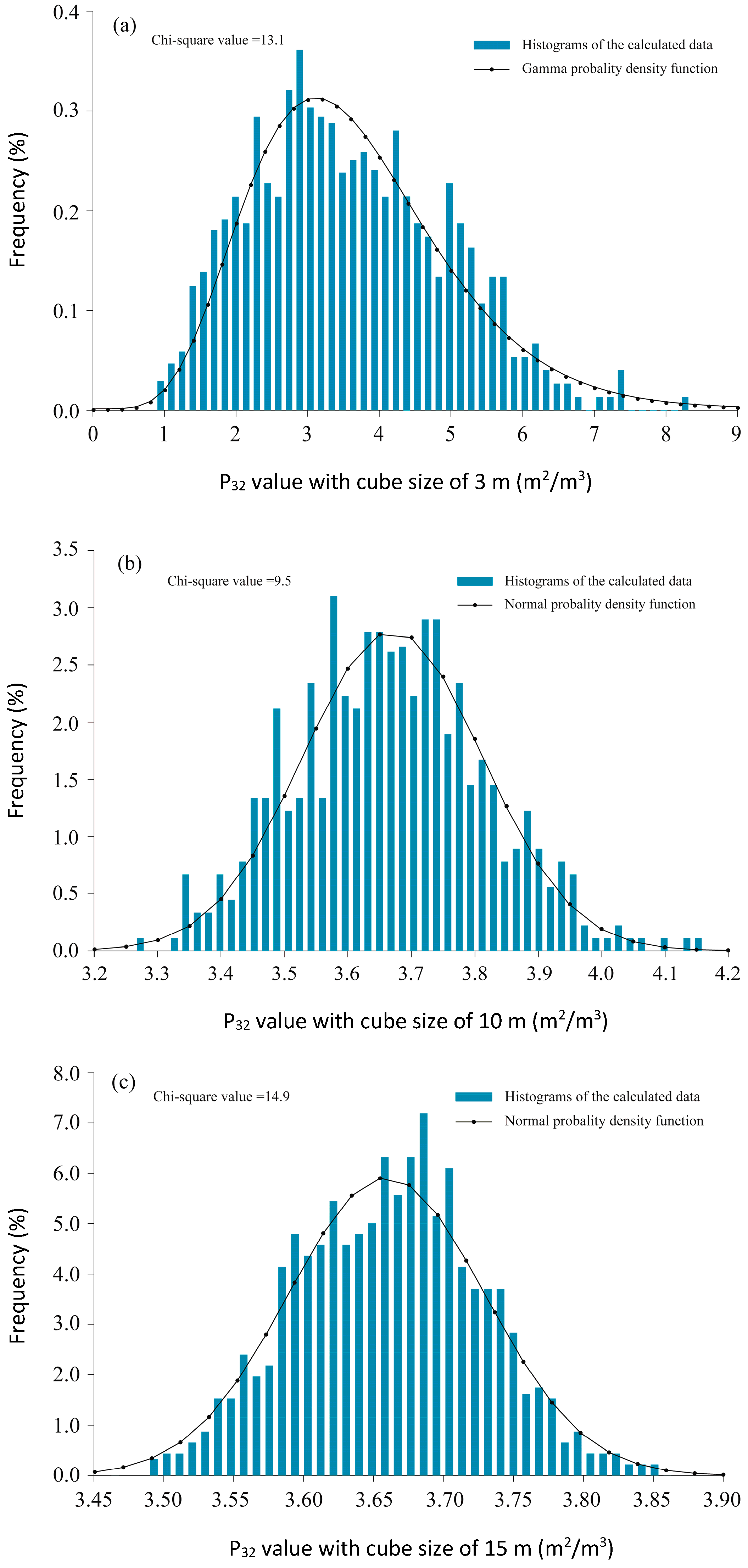
| 3 | 21.0 | 13.1 | Gamma | 13 | 21.0 | 18.7 | Normal |
| 4 | 21.0 | 16.9 | Lognormal | 14 | 21.0 | 13.1 | Normal |
| 5 | 21.0 | 10.9 | Lognormal | 15 | 21.0 | 14.9 | Normal |
| 6 | 21.0 | 11.3 | Lognormal | 16 | 21.0 | 12.3 | Lognormal |
| 7 | 21.0 | 11.2 | Lognormal | 17 | 21.0 | 10.5 | Lognormal |
| 8 | 21.0 | 16.1 | Normal | 18 | 19.7 | 6.3 | Triangle |
| 9 | 21.0 | 8.6 | Lognormal | 19 | 19.7 | 14.4 | Triangle |
| 10 | 21.0 | 9.5 | Normal | 20 | 19.7 | 11.2 | Triangle |
| Cube Size of Sample (m) | Cube Size of Sample 20 (m) | Likelihood Ratio Test | Wald–Wolfowitz Runs Test | ||
|---|---|---|---|---|---|
| p Value | Result | p Value | Result | ||
| 1 | 20 | 7.48 × 10−76 | Reject | 4.49 × 10−64 | Reject |
| 2 | 20 | 4.50 × 10−90 | Reject | 3.43 × 10−44 | Reject |
| 3 | 20 | 2.26 × 10−117 | Reject | 3.46 × 10−39 | Reject |
| 4 | 20 | 9.24 × 10−116 | Reject | 3.46 × 10−39 | Reject |
| 5 | 20 | 1.56 × 10−84 | Reject | 1.37 × 10−37 | Reject |
| 6 | 20 | 1.68 × 10−47 | Reject | 1.70 × 10⁻³⁴ | Reject |
| 7 | 20 | 3.44 × 10−55 | Reject | 9.13 × 10⁻²⁵ | Reject |
| 8 | 20 | 1.99 × 10⁻¹⁵ | Reject | 9.95 × 10⁻²⁹ | Reject |
| 9 | 20 | 4.06 × 10⁻¹⁷ | Reject | 1.30 × 10⁻⁹ | Reject |
| 10 | 20 | 5.72 × 10⁻⁹ | Reject | 7.09 × 10⁻⁹ | Reject |
| 11 | 20 | 5.76 × 10⁻⁵ | Reject | 1.14 × 10⁻⁴ | Reject |
| 12 | 20 | 0.059 | Accept | 0.001 | Reject |
| 13 | 20 | 0.136 | Accept | 0.500 | Accept |
| 14 | 20 | 0.154 | Accept | 0.285 | Accept |
| 15 | 20 | 0.423 | Accept | 0.976 | Accept |
| 16 | 20 | 0.594 | Accept | 0.715 | Accept |
| 17 | 20 | 0.899 | Accept | 0.899 | Accept |
| 18 | 20 | 0.809 | Accept | 0.844 | Accept |
| 19 | 20 | 0.877 | Accept | 0.761 | Accept |
© 2018 by the authors. Licensee MDPI, Basel, Switzerland. This article is an open access article distributed under the terms and conditions of the Creative Commons Attribution (CC BY) license (http://creativecommons.org/licenses/by/4.0/).
Share and Cite
Liu, Y.; Wang, Q.; Chen, J.; Song, S.; Zhan, J.; Han, X. Determination of Geometrical REVs Based on Volumetric Fracture Intensity and Statistical Tests. Appl. Sci. 2018, 8, 800. https://doi.org/10.3390/app8050800
Liu Y, Wang Q, Chen J, Song S, Zhan J, Han X. Determination of Geometrical REVs Based on Volumetric Fracture Intensity and Statistical Tests. Applied Sciences. 2018; 8(5):800. https://doi.org/10.3390/app8050800
Chicago/Turabian StyleLiu, Ying, Qing Wang, Jianping Chen, Shengyuan Song, Jiewei Zhan, and Xudong Han. 2018. "Determination of Geometrical REVs Based on Volumetric Fracture Intensity and Statistical Tests" Applied Sciences 8, no. 5: 800. https://doi.org/10.3390/app8050800
APA StyleLiu, Y., Wang, Q., Chen, J., Song, S., Zhan, J., & Han, X. (2018). Determination of Geometrical REVs Based on Volumetric Fracture Intensity and Statistical Tests. Applied Sciences, 8(5), 800. https://doi.org/10.3390/app8050800