Multi-View Ground-Based Cloud Recognition by Transferring Deep Visual Information


1
Tianjin Key Laboratory of Wireless Mobile Communications and Power Transmission, Tianjin Normal University, Tianjin 300387, China
2
The State Key Laboratory of Management and Control for Complex Systems, Institute of Automation, Chinese Academy of Sciences, Beijing 100190, China
3
The Meteorological Observation Centre, China Meteorological Administration, Beijing 100081, China
*
Author to whom correspondence should be addressed.
Appl. Sci. 2018, 8(5), 748; https://doi.org/10.3390/app8050748
Submission received: 4 April 2018
/
Revised: 4 May 2018
/
Accepted: 5 May 2018
/
Published: 9 May 2018
(This article belongs to the Special Issue Advanced Intelligent Imaging Technology)
Abstract
:Since cloud images captured from different views possess extreme variations, multi-view ground-based cloud recognition is a very challenging task. In this paper, a study of view shift is presented in this field. We focus both on designing proper feature representation and learning distance metrics from sample pairs. Correspondingly, we propose transfer deep local binary patterns (TDLBP) and weighted metric learning (WML). On one hand, to deal with view shift, like variations of illuminations, locations, resolutions and occlusions, we first utilize cloud images to train a convolutional neural network (CNN), and then extract local features from the part summing maps (PSMs) based on feature maps. Finally, we maximize the occurrences of regions for the final feature representation. On the other hand, the number of cloud images in each category varies greatly, leading to the unbalanced similar pairs. Hence, we propose a weighted strategy for metric learning. We validate the proposed method on three cloud datasets (the MOC_e, IAP_e, and CAMS_e) that are collected by different meteorological organizations in China, and the experimental results show the effectiveness of the proposed method.
1. Introduction
Clouds are aerosols consisting of large amounts of frozen crystals, minute liquid droplets, or particles suspended in the atmosphere (https://www.weather.gov/). Their size, type, composition and movement reflect the atmospheric motion. Especially the cloud type, as one of crucial cloud macroscopic parameters in the cloud observation, plays a vital role in the weather prediction and climate change research [1]. Currently, a large quantity of labor and material resources are consumed because ground-based cloud images are classified by qualified professionals. Therefore, developing automatic techniques for ground-based cloud recognition is vital. To date, there are various devices for digitizing ground-based clouds, for example the whole sky imager (WSI) [2], the infrared cloud imager (ICI) [3], and the whole-sky infrared cloud-measuring system (WSIRCMS) [4] etc. With the help of these devices, various methods for automatic ground-based cloud recognition [5,6,7] have been proposed. However, the cloud features used in these methods are not discriminative enough to represent cloud images.
Practically, the appearance of clouds can be regarded as a type of natural texture [8]. Hence making it reasonable to use texture descriptors to portray cloud appearances. Inspired by the success of local features in the texture recognition field [9,10,11,12], some local features are proposed to recognize ground-based cloud images [13,14]. This kind of method includes two procedures; initially, the cloud image is described as a feature vector using local features. Secondly, the Euclidean distance or chi-square distance is utilized in the matching or recognizing process.
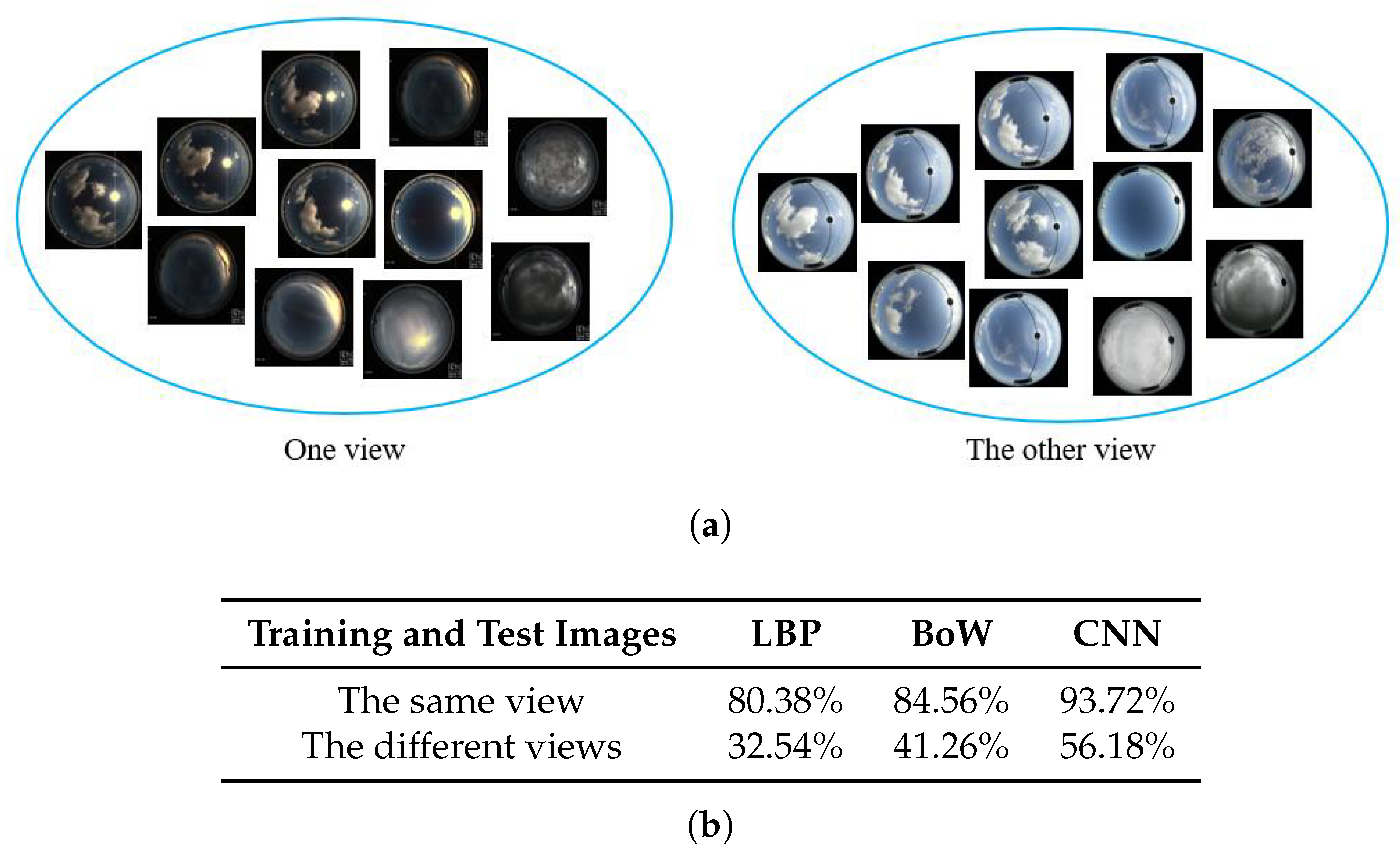
The major focal point of the existing methods is based on recognizing cloud images which originate from similar views. These methods are implemented under the condition that the training and test images come from the same feature space. Nevertheless, these methods are not suitable for multi-view cases. This is because the cloud images captured from different views belong to different feature spaces. Practically, we often handle cloud images in two views. For instance, the cloud images collected by a variety of weather stations possess variances in image resolutions, illuminations, camera settings, occlusions and so on. This kind of cloud images actually distributes in different feature spaces. As illustrated in Figure 1a, the cloud images are captured in multiple views, and vary greatly in appearance. The competitive methods for ground-based cloud recognition, i.e., local binary patterns (LBP) [15], the bag-of-words (BoW) model [16], and the convolutional neural network (CNN) [17], generally achieve promising results when training and testing in the same feature space, while the performances degrade significantly when training and testing in different feature spaces, as shown in Figure 1b. Therefore, we hope to employ cloud images from one view (feature space) to train a classifier, which is then used to recognize cloud images from other views (feature spaces). This is a kind of view shift problem, and we define it as the multi-view ground-based cloud recognition. It is very common worldwide. For instance, for the sake of obtaining completed weather information, it is essential to set up more new weather stations to capture cloud images. However, due to the fact that there are insufficient labelled cloud images in the new weather stations to train a robust classifier makes it unrealistic to expect users to label the cloud images for new weather stations. This is time-consuming and a dissipate of manpower. Considering that there are many labelled cloud images accumulated in the established weather stations, we aspire to employ such labelled cloud images to train a classifier which can be used to recognize cloud images in new weather stations.
In this paper, we propose a novel multi-view ground-based cloud recognition method by transferring deep visual information. The cloud features used in the existing methods are not discriminative enough to sufficiently describe cloud images when presented with view shift, and therefore we propose an effective method named transfer deep local binary patterns (TDLBP) for feature representation. Concretely, we first train a CNN model, and we propose part summing maps (PSMs) based on all feature maps for one convolutional layer. Then we extract LBP in local regions from the PSMs, and each local region is represented as a histogram. Finally, in order to adapt view shift, we discover the maximum occurrence to make a stable representation.
After cloud images are represented as feature vectors, we compute the similarity between feature vectors to classify ground-based cloud images. Classical distance metrics are predefined, such as the Euclidean distance [18], chi-square metric [13] and quadratic-chi metric [19]. Hence, we propose a learning-based method called weighted metric learning (WML) which aims to utilize sample pairs to learn a transformation matrix. In Figure 2, green and blue indicate two kinds of feature spaces. Two samples from both feature spaces comprise a sample pair. Here, the red lines denote similar pairs, while black lines denote dissimilar pairs. In practice, the number of cloud images in each category greatly differs. For example, there are many clear sky images as the clear sky appears frequently, while there are few images of altocumulus which has a low probability of occurrence. There exists an unbalance problem of sample pairs when we learn the transformation matrix. Hence, to avoid the learning process being dominated by sample pairs in which clouds appear frequently, and neglecting limited sample pairs in which clouds occur rarely, we propose a weighted strategy for metric learning. We assign a corresponding weight for sample pairs in each category. Thus, we assign a small weight to sample pairs that possess a large number (squares in Figure 2) and assign a large weight to sample pairs that possess a small number (circles in Figure 2). Finally, we utilize the nearest neighborhood classifier, where the distances are determined by the proposed distance metric, to classify cloud images which are from another feature space.
The rest of this paper is organized as follows. Section 2 presents the related work including feature representation for ground-based cloud recognitions and metric learning. The details of the proposed TDLBP and WML are introduced in Section 3. In Section 4, we conduct a series of experiments to verify the proposed method. Section 5 summarizes the paper.
2. Related Work
In recent years, researchers have developed a number of algorithms for ground-based cloud recognition. The co-occurrence matrix and edge frequency were introduced in [5] to extract local features to describe cloud images, and recognized five different sky conditions. The work [20] extended to classify cloud images into eight sky conditions by utilizing Fourier transformation and statistical features. Since the BoW model is an effective algorithm for texture recognition, some extension methods [21,22] were proposed. Since the appearance of clouds is a kind of natural texture, Sun et al. [23] employed LBP to classify infrared cloud images. Liu et al. [19] proposed illumination-invariant completed local ternary patterns (ICLTP), which can effectively handle the illumination variations. They soon proposed the salient LBP (SLBP) [13] to capture descriptive cloud information. The desirable property of SLBP is the robustness to noises. However, these features are not robust to view shift for describing cloud images.
Recently, due to the inspiration caused by the success of convolutional neural networks (CNNs) in image recognition [17,24], Ye et al. [25] first proposed to apply CNNs to ground-based cloud recognition. They employed Fisher Vector (FV) to encode the last conventional layer of CNNs, and they further proposed to extract the deep convolutional visual features to represent cloud images in [26]. Shi et al. [27] employed the deep convolutional activations-based features (DCAFs) to describe cloud images. These aformentioned methods showed promising recognition results when trained and tested on the same feature space. In other words, these features are also not robust to view shift.
In the recognition procedure to compute similarities or distances between two feature vectors, many predefined metrics cannot show the desirable topology that we are trying to capture. A sought-after alternative is to apply metric learning in place of these predefined metrics. The key idea of metric learning is to conduct a Mahalanobis distance where a transformation matrix is applied to compute the distance between a sample pair. Since metric learning has shown remarkable performance in various fields, such as image retrieval and classification [28], face recognition [29,30,31] and human activity recognition [32,33], we employ the framework of metric learning to ground-based cloud recognition and meanwhile consider the sample imbalance problem.
3. Approach
3.1. Part Summing Maps
With the appearance of large-scale image datasets and the development of high-performance computing systems, CNNs have shown promising performance in image classification [34] and object detection [35,36]. Hence, we extract features from a CNN model to describe cloud images. Generally, an effective CNN requires a large number of training images. When there are insufficient training images to train a CNN, it results in overfitting. In this tribulation, we fine-tune the VGG-19 model [17] on our cloud datasets to train a CNN. As presented in Table 1, the VGG-19 model consists of 16 convolutional layers and three fully-connected (FC) layers. The size of receipt fields throughout the whole model is set to pixels, and the number of receipt fields is different for each convolutional layer. In the process of fine-tuning the VGG-19 model, we replace the number of kernels in the final FC layer with the number of cloud categories.
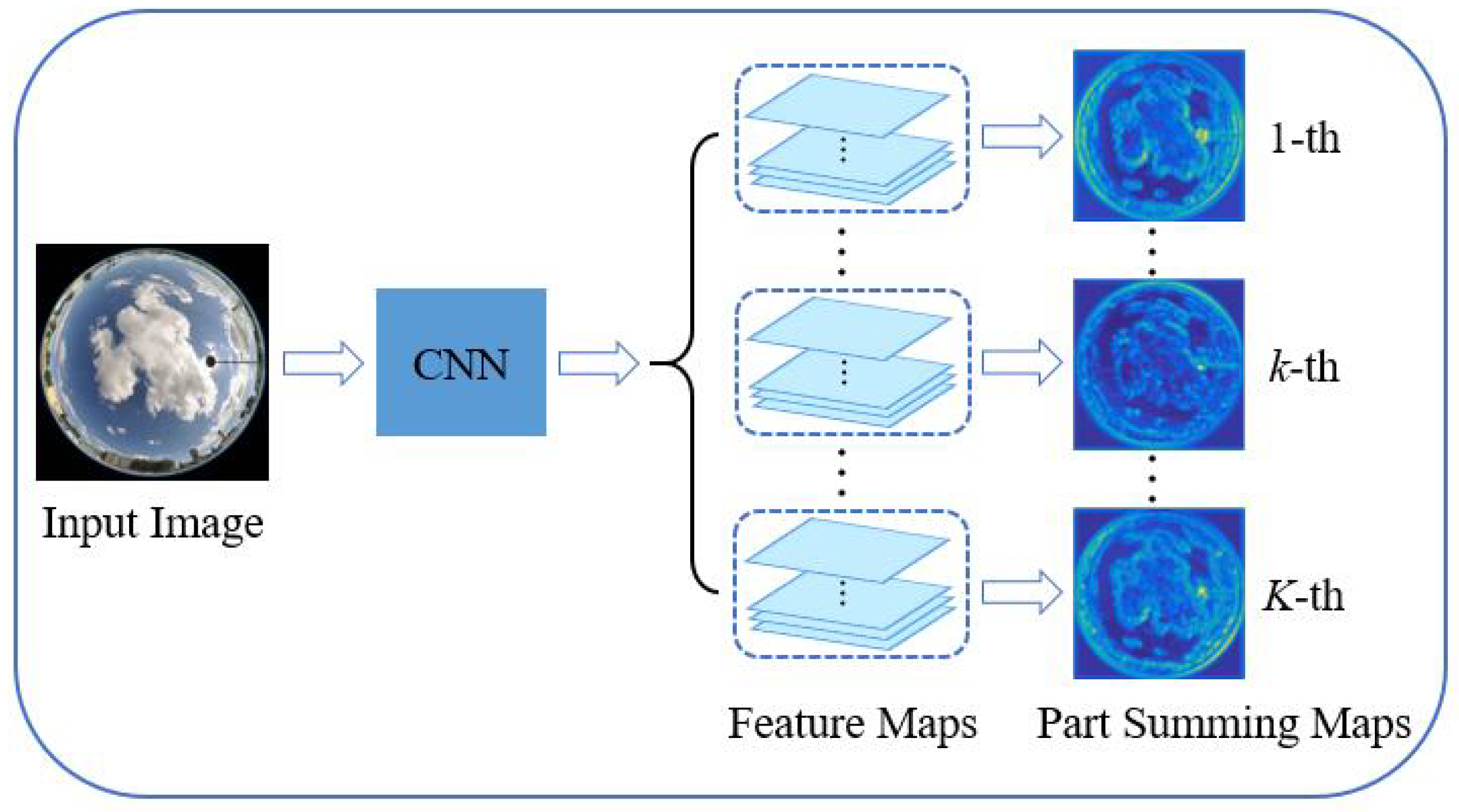
A lot of processes have been developed in utilizing feature maps for image representations in computer vision fields [37,38,39]. Furthermore, the feature maps for a convolutional layer describe different patterns. To obtain completed information from the convolutional layer, we propose PSMs based on all feature maps for image representations. Practically, we divide all feature maps from one convolutional layer into several parts for one cloud image evenly. Suppose that there are K parts of feature maps, as shown in Figure 3. Then we add the feature maps of each part into one part summing map (PSM), denoted as , and it is formulated as:
where indicates the j-th feature map and J is the number of the feature maps in each part.
3.2. Transfer Deep LBP
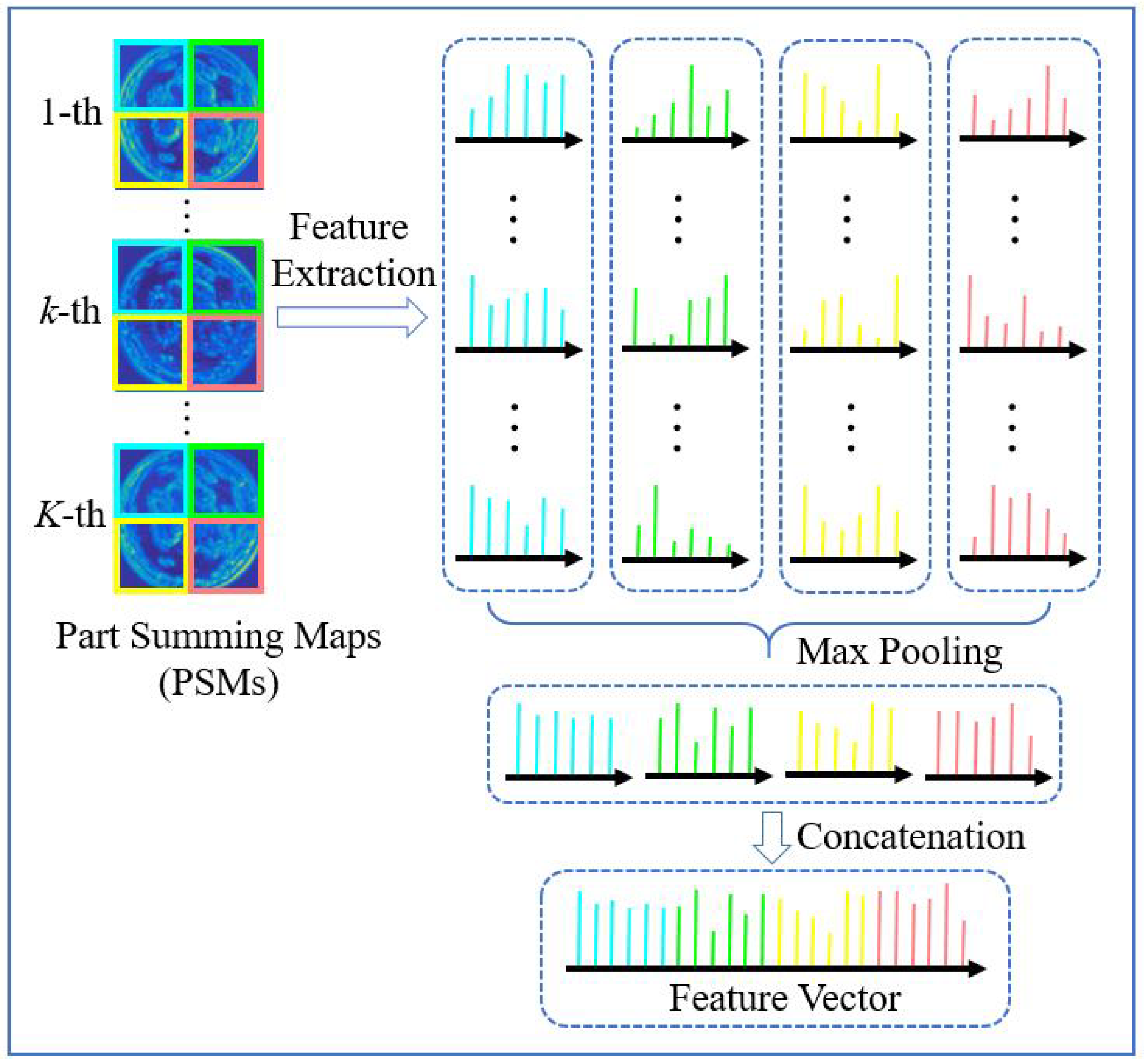
We propose TDLBP to address the view shift problem. The convolutional layers can capture more local characteristics [40,41]. Therefore, we propose to extract local patterns from the PSMs of a convolutional layer to represent cloud images. TDLBP is an improved operator over LBP, which computes a region representation based on the PSMs. The TDLBP is not only invariance to intensity scale changes, but is robust to view shift and obtain the completed scale information of cloud. We first partition each PSM into (L = 1, 2, 3) regions. Second, we extract LBP in each region of the PSMs. We take the PSMs of regions as an example (see Figure 4) and perform the following steps:
- (1)
- Feature extractions for each region in the PSMs. Within each region, we extract three scales of LBP histograms, i.e., = (8, 1), (16, 2) and (24, 3). Hence, each region can be described as a 54 dimensional descriptor.
- (2)
- Feature pooling. Max pooling is applied on all local features of the local regions at the same position, i.e., preserving the maximum value of each bin among all histograms, resulting in four histograms. The pooled feature of each local region is more robust to view shift.
- (3)
- Feature concatenation. The four histograms are concatenated into one histogram to represent each cloud image. The resulting histogram can capture global information and local characteristics of image regions, simultaneously.
3.3. Weighted Metric Learning
Suppose there is a sample pair , where and are the feature vectors of two cloud images from two views, respectively (i.e., i and z come from two feature spaces). If the category labels of i and z are the same (or different), we define as a similar pair (dissimilar pair). The number of cloud categories from each view is N, and we further construct N sets of similar pairs:
where is a set of similar pairs in the n-th category. We formulate the dissimilar pairs as:
We aspire to learn a transformation matrix () to parameterize the squared Mahalanobis distance:
where is a positive semidefinite matrix. For convenience, we denote . The squared Mahalanobis distance is a scalar, and hence we reformulate Equation (4) as:
Our goal is to minimize the distance between similar pairs, and meanwhile maximize the distance between dissimilar pairs. For this purpose, we conduct the following objective function:
where is the cost function, the distances of all similar pairs are added to obtain , and is the sum of the distances of dissimilar pairs. and are defined in the following. The first constraint ensures a valid metric, and the second one excludes the trivial solution [42].
When computing in the learning process, the classical metric learning methods assign the same weight to each similar pair of all categories. This does not consider that the numbers of similar pairs in each category is largely unbalanced. This weight strategy is not suitable for multi-view ground-based cloud recognition, because the occurrence probabilities of various weather conditions are different, and the number of cloud images in each category varies greatly resulting in the unbalanced similar pairs. Therefore, we propose WML to solve the problem of sample unbalance. For similar pairs, we assign a different weight to each category. Concretely, we first compute the distances between similar pairs of each category, and give a weight to each category according to the similar pair number. Then we sum the weighted distance of all categories. We compute and by:
where is the number of similar pairs in the n-th category, and is the total number of dissimilar pairs of all categories.
We minimize the objective function, i.e., Equation (6), subject to two constraints to learn M. Since is a positive semidefinite matrix, the first constraint can be relaxed when explicitly solved for M [42]. Equations (7) and (8) are substituted into Equation (6), and then we make use of the standard Lagrange multiplier on Equation (6):
Then the partial derivative of the Lagrangian function with respect to M is computed, and we set the result to zero:
where
and
We solve the eigenvalue of Equation (10), and preserve r eigenvectors of corresponding to the first r largest eigenvalues. As a result, the learned transformation matrix M is equal to:
where is the eigenvector of corresponding to the largest eigenvalue, and is the eigenvector of corresponding to the second largest eigenvalue, and so on.
4. Experiments
4.1. Datasets and Experimental Setup
In this paper, each cloud dataset is divided into seven categories according to the criteria published in World Meteorological Organization (WMO). The first cloud dataset MOC_e is collected in Wuxi, Jiangsu Province, China, and provided by Meteorological Observation Centre, China Meteorological Administration. The cloud images have strong illuminations and no occlusions, and have the resolution of . There are two cloud datasets, i.e., the CAMS_e and IAP_e, captured in Yangjiang, Guangdong Province, China, but provided by Chinese Academy of Meteorological Sciences, and Institute of Atmospheric Physics, Chinese Academy of Sciences, respectively. Each cloud image in the CAMS_e is pixels with weak illuminations and no occlusions. The acquisition device used to collect the IAP_e differs from that of the CAMS_e, and as a result, the cloud images from the IAP_e have higher resolution of , strong illuminations and occlusions. The total number of the MOC_e is 2107, and the CAMS_e’s total number is 2491. The IAP_e has a large number of 3533. The number of each category is listed in Table 2. Samples for each category are shown in Figure 5. It is observed that each cloud dataset is captured from different views and belongs to different feature spaces.
All images from the three datasets are resized to pixels, and we employ the feature maps of the fourth convolutional layer. We select two parts of the images as the training images, i.e., all of the images from one view and half of images in each category from another view, and the remaining are taken as the test images. We implement experiments 10 times, and we take the average accuracy over these 10 times as the final results.
4.2. Effect of TDLBP
We compare the proposed TDLBP with the other two texture features, i.e., LBP and DLBP. It should be noted that we extract LBP from the original cloud images and the PSMs, respectively, so we define the second one as DLBP. For fair comparison, we partition all original cloud images (for LBP) and the PSMs (for DLBP and TDLBP) into (L = 1, 2, 3) regions. For each region, we extract three scales LBP with equal to (8, 1), (16, 2) and (24, 3). As for LBP, we accumulate LBP histograms in each divided region, and concatenate all histograms into one histogram with + + = 756 dimensions. As for DLBP, within each region of the PSMs, we extract LBP histograms, and then apply sum pooling to aggregate all features in each region. Each image is also described as a feature vector with 756 dimensions. The chi-square metric is used in this section, and Table 3 presents the recognition accuracies.
From Table 3, in all six situations, the highest classification accuracies are obtained by TDLBP. Both TDLBP and DLBP outperform LBP, because the CNN can learn highly nonlinear features for view shift. Moreover, TDLBP and DLBP are extracted from the PSMs which contain the completed and spatial information of clouds. The TDLBP outperforms DLBP by about 1% in all six situations. Since cloud images have some interferences and noises in general, max pooling could opt for the discriminative and salient features. Hence, TDLBP is more suitable for adapting view shift. Furthermore, the best performance is obtained in the situation of the IAP_e to MOC_e shift. This is probably because the cloud images of IAP_e have some similarities with the ones of MOC_e, such as illuminations, occlusions and locations.
We replaced chi-square metric with metric learning to classify the cloud images with the three features, and we denote them as LBP + ML, DLBP + ML and TDLBP + ML, respectively. From the results shown in Table 4, with the help of metric learning, the performance improvement is more significant, i.e., it all improves approximately by 2%. Particularly, TDLBP + ML achieves the best recognition results in all six conditions. It demonstrates that TDLBP is effective both in predefined metric and learning-based metric. In addition, it is observed that metric learning is more suitable for measuring the similarity between sample pairs when presented with view shift.
4.3. Effect of WML
In this subsection, we evaluate WML combined with the above mentioned features. LBP + WML, DLBP + WML and TDLBP + WML denote LBP, DLBP and TDLBP with the proposed WML, respectively. We choose in Equation (13) when learning M, and the number of PSMs . The results are shown in Table 5 where we can observe that TDLBP + WML achieves the best performance in all multi-view recognitions once again. Comparing Table 5 with Table 4, the proposed WML achieves better results than ML when using the same features, because it considers the imbalanced sample problem by using a weight strategy.
In order to further verify the effectiveness of the WML, we compare WML with SMOTEBoost [43] and RUSBoost [44] based on TDLBP. SMOTEBoost and RUSBoost are the representative methods for alleviating the problem of class sample imbalance where we make use of the default optimal parameters for them. From Table 6, the proposed TDLBP + WML still achieves the best recognition result in all multi-view recognition cases. The performances of SMOTEBoost and RUSBoost are very similar, but RUSBoost is a preferable alternative for learning from imbalanced data because it is simpler, faster, and less complex than SMOTEBoost.
4.4. Comparison to the Competitive Methods
We compare the proposed method TDLBP + WML with three competitive methods, i.e., LBP, BoW and CNN. Note that the experimental results of LBP in this section are the same as the one mentioned in Table 4. For BoW, we stretch a neighborhood around each pixel into an 81 dimensional vector to represent each patch, and apply Weber’s law [45] to normalize the patch vectors. Then, we learn a dictionary for each category by using K-means clustering [46] over patch vectors, and the size of dictionary for each category is set to 300. Each image is described as a 2100 dimensional vector. Finally, we make use of LIBSVM [47] for SVM training and classification with the radial basis function (RBF) kernel, where the parameters C and are set to 200 and 2, respectively. The C is a penalty coefficient that trades off the relationship between the misclassification and the complexity of the decision surface. The is a parameter of the RBF kernel, and can be seen as the inverse of the radius of influence of samples selected by the model as support vectors. For CNN, we utilize the widely-used VGG-19 model [17] for fine-tuning the network on the cloud datasets. Then we treat the final FC layer as the feature vector. Note that LBP, BoW and CNN utilize the same training samples as TDLBP + WML.
From the experimental results listed in Table 7, LBP, BoW and CNN are not suitable for multi-view ground-based cloud recognition. However, BoW and CNN still outperform LBP, because LBP is a fixed feature extraction method without learning process. Compared with BoW and CNN, we not only extract the feature vectors from PSMs, but also sufficiently consider the diverse numbers of cloud images in each category. Hence, the proposed method outperforms BoW and CNN by more than 30% and 17%, respectively.
4.5. Influence of Parameter Variances
In this section, we analyze the proposed TDLBP + WML in three aspects, including the selection of the convolutional layers for PSMs, and the influences of K and r. It is noted that we select the IAP_e as one view, and the MOC_e as the other view to implement the following experiments.
Generally, we can extract structural and textural local features from shallow convolutional layers of a CNN, and extract features with high-level semantic information from deep convolutional layers. The appearance of clouds can be regarded as a type of natural texture, and therefore we extract feature from the PSMs in the shallow convolutional layers. We select the first to eighth convolutional layers for the PSMs to analyze the performance of TDLBP + WML. From Table 8, it is obvious that the highest result of TDLBP + WML is obtained when we make use of the PSMs in the 4-th convolutional layer.
Since each convolutional layer contains different information, we extract TDLBP features from two different convolutional layers for cloud image representation in order to obtain the completed cloud information. From Table 9, TDLBP + WML obtains the highest result when utilizing the PSMs of , and therefore we combine with each of the other convolutional layers for TDLBP feature extraction. Specifically, we extract TDLBP features from this kind of two convolutional layer, and the resulting TDLBP features are concatenated to form the final feature for describing the cloud image. Comparing Table 9 with Table 8, the performances all improve, and the case of achieves the best result of 79.46%. Based on this result, we further combine TDLBP features for three different convolutional layers, and follow the same procedure of feature extraction as mentioned above. The results are shown in Table 10. Comparing Table 10 with Table 9, the performances slightly degrade. Hence, considering both the computation complexity and the recognition accuracy, we conclude that extracting TDLBP features from two different convolutional layers is optimal for cloud image representation.
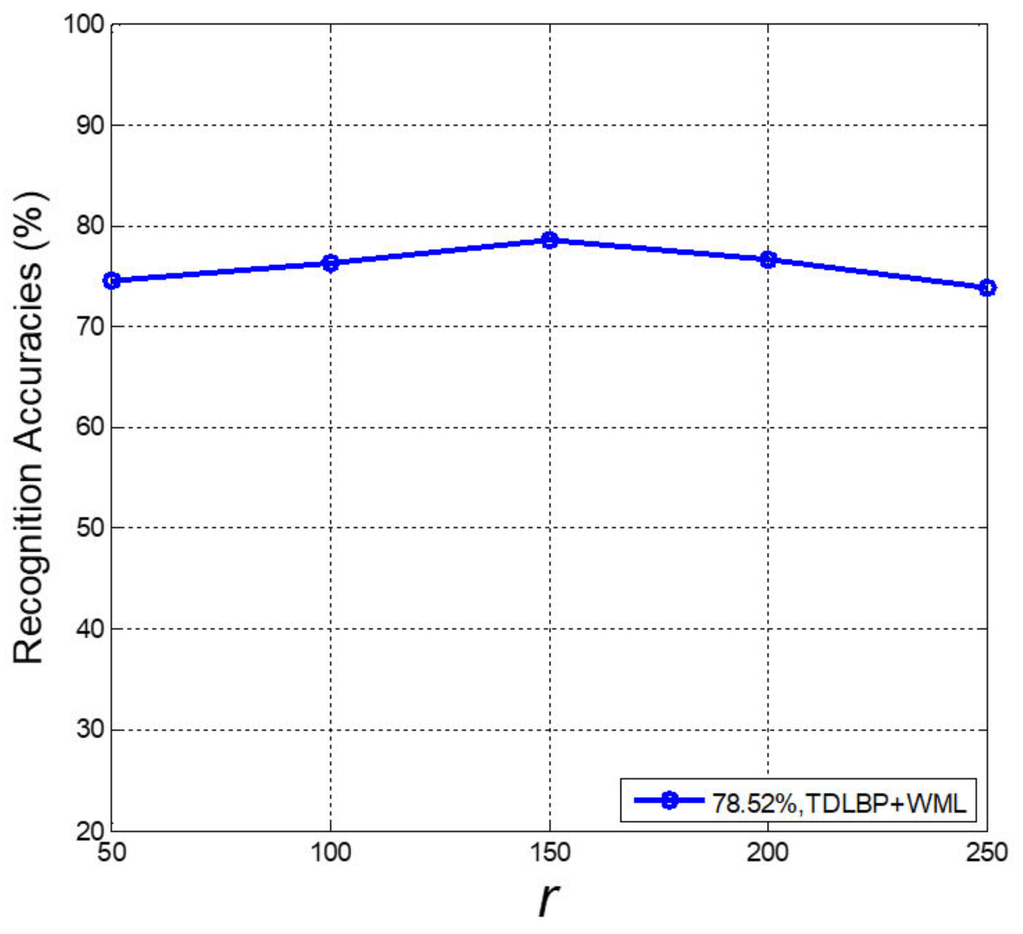
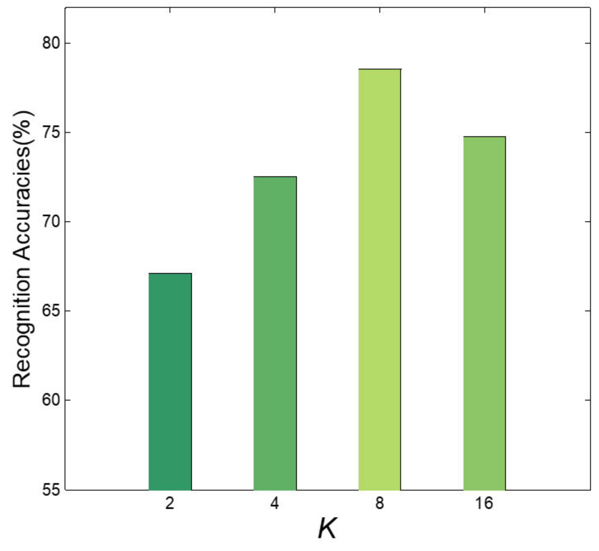
The effect of K on recognition performance is shown in Figure 6, and K is the number of PSMs for the 4-th convolutional layer. We can conclude that larger K may result in better recognition accuracies, but may probably lead to heavier computational burden. We obtain the best result when K increases to 8. r is the the number of eigenvalues (see Section 3.3). r has an impact on recognition performance as it controls the dimensionality of M. In addition, we evaluate the performance of TDLBP + WML with respect to r. As illustrated in Figure 7, with r increasing, the recognition performance improves, and the best result of 78.52% is obtained at a certain point where r is equal to 150. The proper r can make the feature vectors contain the discriminative information with the favourable dimensionality.
5. Conclusions
In conclusion, we have proposed TDLBP + WML for multi-view ground-based cloud recognition. Specifically, a novel feature representation called TDLBP has been proposed which is robust to view shift, such as variances in locations, illuminations, resolutions and occlusions. Furthermore, since the numbers of cloud images in each category is different, we propose WML which assigns different weights to each category when learning the transformation matrix. We have verified TDLBP + WML with a series of experiments on three cloud datasets, i.e., the MOC_e, CAMS_e, and IAP_e. Compared to other competitive methods, TDLBP + WML achieves better performance.
Author Contributions
All authors made significant contributions to the manuscript. Z.Z. and D.L. conceived, designed and performed the experiments, and wrote the paper; S.L. performed the experiments and analyzed the data; B.X. and X.C. provided the background knowledge of cloud classification and gave constructive advices.
Acknowledgments
This work was supported by National Natural Science Foundation of China under Grant No. 61501327 and No. 61711530240, Natural Science Foundation of Tianjin under Grant No. 17JCZDJC30600 and No. 15JCQNJC01700, the Fund of Tianjin Normal University under Grant No.135202RC1703, the Open Projects Program of National Laboratory of Pattern Recognition under Grant No. 201700001 and No. 201800002, the China Scholarship Council No. 201708120039 and No. 201708120040, and the Tianjin Higher Education Creative Team Funds Program.
Conflicts of Interest
The authors declare no conflict of interest.
References
- Chen, Z.; Zen, D.; Zhang, Q. Sky model study using fuzzy mathematics. J. Illum. Eng. Soc. 1994, 23, 52–58. [Google Scholar] [CrossRef]
- Shields, J.E.; Karr, M.E.; Tooman, T.P.; Sowle, D.H.; Moore, S.T. The whole sky imager—A year of progress. In Proceedings of the Eighth Atmospheric Radiation Measurement Science Team Meeting, Tucson, AZ, USA, 23–27 March 1998; pp. 23–27. [Google Scholar]
- Shaw, J.A.; Thurairajah, B.; Edqvist, E.; Mizutan, K. Infrared cloud imager deployment at the north slope of Alaska during early 2002. In Proceedings of the Twelfth Atmospheric Radiation Measurement Science Team Meeting, St. Petersburg, FL, USA, 8–12 April 2002; pp. 1–7. [Google Scholar]
- Sun, X.J.; Gao, T.C.; Zhai, D.L.; Zhao, S.J.; Lian, J.G. Whole sky infrared cloud measuring system based on the uncooled infrared focal plane array. Infrared Laser Eng. 2008, 37, 761–764. [Google Scholar]
- Singh, M.; Glennen, M. Automated ground-based cloud recognition. Pattern Anal. Appl. 2005, 8, 258–271. [Google Scholar] [CrossRef]
- Calbo, J.; Sabburg, J. Feature extraction from whole-sky ground-based images for cloud-type recognition. J. Atmos. Ocean. Technol. 2008, 25, 3–14. [Google Scholar] [CrossRef]
- Heinle, A.; Macke, A.; Srivastav, A. Automatic cloud classification of whole sky images. Atmos. Meas. Tech. 2010, 3, 557–567. [Google Scholar] [CrossRef] [Green Version]
- Pentland, A.P. Fractal-based description of natural scenes. IEEE Trans. Pattern Anal. Mach. Intell. 1984, 6, 661–674. [Google Scholar] [CrossRef] [PubMed]
- Varma, M.; Zisserman, A. A statistical approach to texture classification from single images. Int. J. Comput. Vis. 2005, 62, 61–81. [Google Scholar] [CrossRef]
- Varma, M.; Zisserman, A. A statistical approach to material classification using image patch exemplars. IEEE Trans. Pattern Anal. Mach. Intell. 2009, 31, 2032–2047. [Google Scholar] [CrossRef] [PubMed]
- Zakeri, H.; Yamazaki, F.; Liu, W. Texture Analysis and Land Cover Classification of Tehran Using Polarimetric Synthetic Aperture Radar Imagery. Appl. Sci. 2017, 7, 452. [Google Scholar] [CrossRef]
- Liu, L.; Fieguth, P.; Guo, Y.; Wang, X.; Pietikäinen, M. Local binary features for texture classification: Taxonomy and experimental study. Pattern Recogn. 2017, 62, 135–160. [Google Scholar] [CrossRef]
- Liu, S.; Wang, C.; Xiao, B.; Zhang, Z.; Shao, Y. Salient local binary pattern for ground-based cloud classification. Acta Meteorol. Sin. 2013, 27, 211–220. [Google Scholar] [CrossRef]
- Kliangsuwan, T.; Heednacram, A. Feature extraction techniques for ground-based cloud type classification. Expert Syst. Appl. 2015, 42, 8294–8303. [Google Scholar] [CrossRef]
- Ojala, T.; Pietikainen, M.; Maenpaa, T. Multiresolution gray-scale and rotation invariant texture classification with local binary patterns. IEEE Trans. Pattern Anal. Mach. Intell. 2002, 24, 971–987. [Google Scholar] [CrossRef]
- Leung, T.; Malik, J. Representing and recognizing the visual appearance of materials using three-dimensional textons. Int. J. Comput. Vis. 2001, 43, 29–44. [Google Scholar] [CrossRef]
- Simonyan, K.; Zisserman, A. Very deep convolutional networks for large-scale image recognition. In Proceedings of the International Conference on Learning Representations, San Diego, CA, USA, 7–9 May 2015; pp. 7–9. [Google Scholar]
- Wang, L.; Zhang, Y.; Feng, J. On the Euclidean distance of images. IEEE Trans. Pattern Anal. Mach. Intell. 2005, 27, 1334–1339. [Google Scholar] [CrossRef] [PubMed]
- Liu, S.; Wang, C.; Xiao, B.; Zhang, Z.; Shao, Y. Illumination-invariant completed LTP descriptor for cloud classification. In Proceedings of the 5th International Congress on Image and Signal Processing, Chongqing, China, 16–18 October 2012; pp. 449–453. [Google Scholar]
- Long, C.N.; Sabburg, J.M.; Calbó, J.; Pagès, D. Retrieving cloud characteristics from ground-based daytime color all-sky images. J. Atmos. Ocean. Technol. 2006, 23, 633–652. [Google Scholar] [CrossRef]
- Liu, S.; Wang, C.; Xiao, B.; Zhang, Z.; Shao, Y. Soft-signed sparse coding for ground-based cloud classification. In Proceedings of the International Conference on Pattern Recognition, Tsukuba Science City, Japan, 11–15 November 2012; pp. 2214–2217. [Google Scholar]
- Liu, S.; Wang, C.; Xiao, B.; Zhang, Z.; Shao, Y. Ground-based cloud classification using multiple random projections. In Proceedings of the International Conference on Computer Vision in Remote Sensing, Xiamen, China, 16–18 December 2012; pp. 7–12. [Google Scholar]
- Sun, X.J.; Liu, L.; Gao, T.C.; Zhao, S.J. Classification of whole sky infrared cloud image based on the LBP operator. Trans. Atmos. Sci. 2009, 32, 490–497. [Google Scholar]
- Ren, S.; He, K.; Girshick, R.; Sun, J. Faster R-CNN: Towards real-time object detection with region proposal networks. In Proceedings of the Advances in Neural Information Processing Systems, Montreal, QC, Canada, 7–12 December 2015; pp. 91–99. [Google Scholar]
- Ye, L.; Cao, Z.; Xiao, Y.; Li, W. Ground-based cloud image categorization using deep convolutional visual features. In Proceedings of the IEEE International Conference on Image Processing, Quèbec City, QC, Canada, 27–30 September 2015; pp. 4808–4812. [Google Scholar]
- Ye, L.; Cao, Z.; Xiao, Y. DeepCloud: Ground-based cloud image categorization using deep convolutional features. IEEE Trans. Geosci. Remote Sens. 2017, 55, 5729–5740. [Google Scholar] [CrossRef]
- Shi, C.; Wang, C.; Wang, Y.; Xiao, B. Deep convolutional activations-based features for ground-based cloud classification. IEEE Geosci. Remote Sens. Lett. 2017, 14, 816–820. [Google Scholar] [CrossRef]
- Kulis, B.; Jain, P.; Grauman, K. Fast similarity search for learned metrics. IEEE Trans. Pattern Anal. Mach. Intell. 2009, 31, 2143–2157. [Google Scholar] [CrossRef] [PubMed]
- Guillaumin, M.; Verbeek, J.; Schmid, C. Is that you? Metric learning approaches for face identification. In Proceedings of the International Conference on Computer Vision, Kyoto, Japan, 27 September–4 October 2009; pp. 498–505. [Google Scholar]
- Lu, J.; Wang, G.; Moulin, P. Localized multifeature metric learning for image-set-based face recognition. IEEE Trans. Circuits Syst. Video Technol. 2016, 26, 529–540. [Google Scholar] [CrossRef]
- Saxena, S.; Verbeek, J. Heterogeneous face recognition with CNNs. In Proceedings of the European Conference on Computer Vision, Amsterdam, The Netherlands, 8–16 October 2016; pp. 483–491. [Google Scholar]
- Tran, D.; Sorokin, A. Human activity recognition with metric learning. In Proceedings of the European Conference on Computer Vision, Marseille, France, 12–18 October 2008; pp. 548–561. [Google Scholar]
- Zhang, Z.; Wang, C.; Xiao, B.; Zhou, W.; Liu, S.; Shi, C. Cross-view action recognition via a continuous virtual path. In Proceedings of the IEEE Conference on Computer Vision and Pattern Recognition, Portland, OR, USA, 23–28 June 2013; pp. 2690–2697. [Google Scholar]
- Krizhevsky, A.; Sutskever, I.; Hinton, G.E. Imagenet classification with deep convolutional neural networks. In Proceedings of the Advances In Neural Information Processing Systems, Lake Tahoe, NV, USA, 3–6 December 2012; pp. 1097–1105. [Google Scholar]
- Ren, S.; He, K.; Girshick, R.; Zhang, X.; Sun, J. Object detection networks on convolutional feature maps. IEEE Trans. Pattern Anal. Mach. Intell. 2017, 39, 1476–1481. [Google Scholar] [CrossRef] [PubMed]
- Rizvi, S.; Tahir, H.; Cabodi, G.; Francini, G. Optimized Deep Neural Networks for Real-Time Object Classification on Embedded GPUs. Appl. Sci. 2017, 7, 826. [Google Scholar] [CrossRef]
- Babenko, A.; Lempitsky, V. Aggregating local deep features for image retrieval. In Proceedings of the IEEE International Conference on Computer Vision, Santiago, Chile, 7–13 December 2015; pp. 1269–1277. [Google Scholar]
- Cimpoi, M.; Maji, S.; Vedaldi, A. Deep filter banks for texture recognition and segmentation. In Proceedings of the IEEE Conference on Computer Vision and Pattern Recognition, Boston, MA, USA, 7–12 June 2015; pp. 3828–3836. [Google Scholar]
- Shi, B.; Wang, X.; Lyu, P.; Yao, C.; Bai, X. Robust scene text recognition with automatic rectification. In Proceedings of the IEEE Conference on Computer Vision and Pattern Recognition, Seattle, WA, USA, 27–30 June 2016; pp. 4168–4176. [Google Scholar]
- Zeiler, M.D.; Fergus, R. Visualizing and understanding convolutional networks. In Proceedings of the European Conference On Computer Vision, Zurich, Switzerland, 6–12 September 2014; pp. 818–833. [Google Scholar]
- Mahendran, A.; Vedaldi, A. Visualizing deep convolutional neural networks using natural pre-images. Int. J. Comput. Vis. 2016, 120, 233–255. [Google Scholar] [CrossRef]
- Alipanahi, B.; Biggs, M.; Ghodsi, A. Distance metric learning vs. Fisher discriminant analysis. In Proceedings of the Conference On Artificial Intelligence, Chicago, IL, USA, 13–17 July 2008; pp. 598–603. [Google Scholar]
- Chawla, N.V.; Lazarevic, A.; Hall, L.O.; Bowyer, K.W. SMOTEBoost: Improving prediction of minority class in boosting. In Proceedings of the European Conference on Principles of Data Mining and Knowledge Discovery, Cavtat-Dubrovnik, Croatia, 22–26 September 2003; pp. 107–119. [Google Scholar]
- Seiffert, C.; Khoshgoftaar, T.M.; Van Hulse, J.; Napolitano, A. RUSBoost: A hybrid approach to alleviating class imbalance. IEEE Trans. Syst. Man Cybern. Part A Syst. Hum. 2010, 40, 185–197. [Google Scholar] [CrossRef]
- Liu, L.; Fieguth, P. Texture classification from random features. IEEE Trans. Pattern Anal. Mach. Intell. 2012, 34, 574–586. [Google Scholar] [CrossRef] [PubMed]
- Lloyd, S. Least squares quantization in PCM. IEEE Trans. Inf. Theory 1982, 28, 129–137. [Google Scholar] [CrossRef]
- Chang, C.-C.; Lin, C.-J. LIBSVM: A library for support vector machines. ACM Trans. Intel. Syst. Technol. 2011, 2, 27. [Google Scholar] [CrossRef]
Figure 1.
(a) We present cloud images from two different views; (b) The performance of three competitive methods degrade when presented with view shift.
Figure 1.
(a) We present cloud images from two different views; (b) The performance of three competitive methods degrade when presented with view shift.

Figure 2.
The green and blue indicate two kinds of feature spaces. Then we employ weighted pairwise constraints to the feature spaces. Here, red and black lines denote similar pairs and dissimilar pairs, respectively. The final feature space is learned for cloud recognition.
Figure 2.
The green and blue indicate two kinds of feature spaces. Then we employ weighted pairwise constraints to the feature spaces. Here, red and black lines denote similar pairs and dissimilar pairs, respectively. The final feature space is learned for cloud recognition.
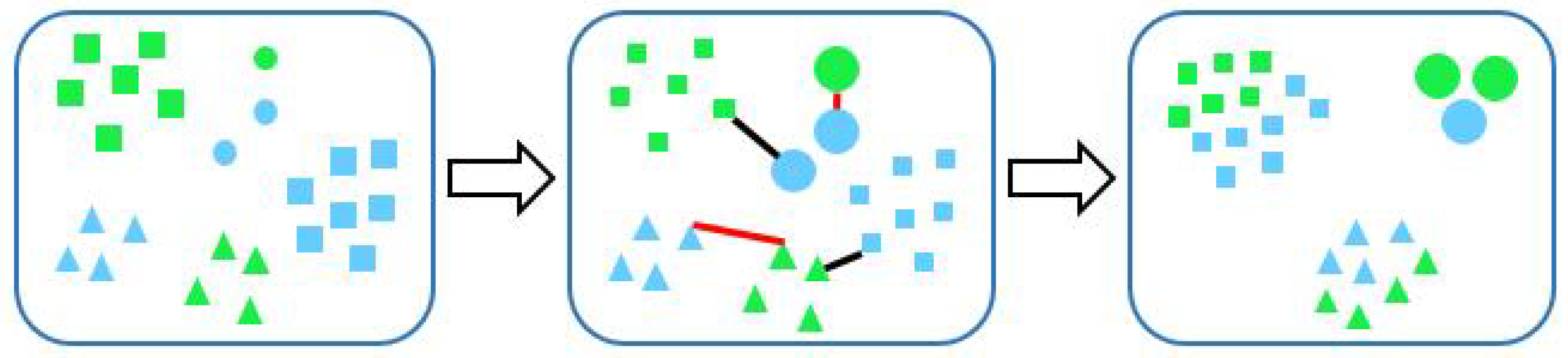
Figure 3.
The procedure of generating part summing maps.

Figure 4.
Each PSM is divided into regions, which are denoted as four colors, i.e., blue, green, yellow, and pink, respectively. We extract features from each region, and apply max pooling for the final feature representation.
Figure 4.
Each PSM is divided into regions, which are denoted as four colors, i.e., blue, green, yellow, and pink, respectively. We extract features from each region, and apply max pooling for the final feature representation.

Figure 5.
We present cloud samples of each category (each row indicates one category) from the three cloud datasets, i.e., (a) the MOC_e, (b) the CAMS_e, and (c) the IAP_e.
Figure 5.
We present cloud samples of each category (each row indicates one category) from the three cloud datasets, i.e., (a) the MOC_e, (b) the CAMS_e, and (c) the IAP_e.
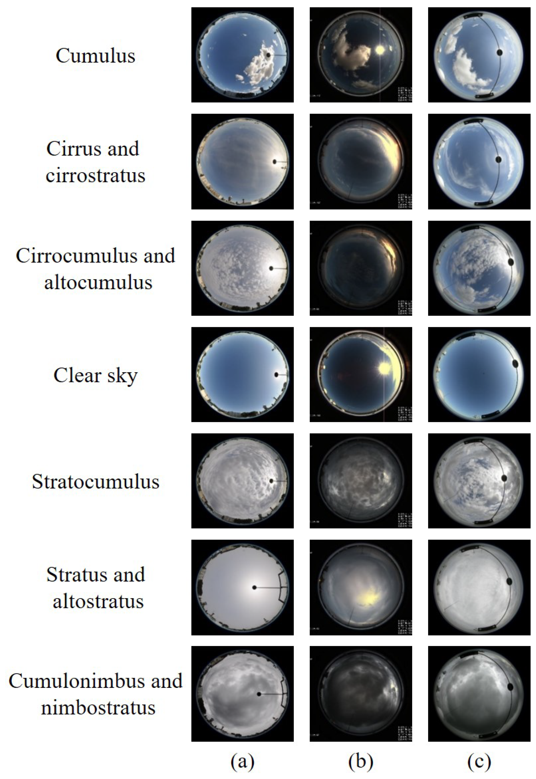
Figure 6.
Recognition accuracies achieved by TDLBP + WML with varied numbers of K.

Figure 7.
Recognition accuracies achieved by TDLBP + WML with varied numbers of r.

Table 1.
The configuration of the VGG-19 model. con_i denotes the i-th convolutional layer, and the convolution stride is set to 1 pixel. Max pooling is implemented by a sliding window of pixels with stride 2.
Table 1.
The configuration of the VGG-19 model. con_i denotes the i-th convolutional layer, and the convolution stride is set to 1 pixel. Max pooling is implemented by a sliding window of pixels with stride 2.
| Config. | The VGG-19 Model |
|---|---|
| conv_1 | |
| conv_2 | |
| max pooling | |
| conv_3 | |
| conv_4 | |
| max pooling | |
| conv_5 | |
| conv_6 | |
| conv_7 | |
| conv_8 | |
| max pooling | |
| conv_9 | |
| conv_10 | |
| conv_11 | |
| conv_12 | |
| max pooling | |
| conv_13 | |
| conv_14 | |
| conv_15 | |
| conv_16 | |
| max pooling | |
| fc_17 | 4096-d |
| fc_18 | 4096-d |
| fc_19 | 1000-d, softmax |
Table 2.
The sample number in each category of three datasets.
| Cloud Category | Number of Cloud Images | ||
|---|---|---|---|
| MOC_e | CAMS_e | IAP_e | |
| Cumulus | 278 | 397 | 1072 |
| Cirrus and cirrostratus | 303 | 373 | 516 |
| Cirrocumulus and altocumulus | 109 | 113 | 32 |
| Clear sky | 302 | 171 | 88 |
| Stratocumulus | 35 | 188 | 536 |
| Stratus and altostratus | 836 | 192 | 679 |
| Cumulonimbus and nimbostratus | 244 | 1057 | 610 |
| Total number | 2107 | 2491 | 3533 |
Table 3.
Multi-view cloud recognition accuracies (%) using different features.
| One View | The Other View | LBP | DLBP | TDLBP |
|---|---|---|---|---|
| MOC_e | CAMS_e | 31.38 | 63.25 | 64.87 |
| MOC_e | IAP_e | 41.24 | 69.56 | 70.85 |
| CAMS_e | IAP_e | 32.54 | 65.18 | 66.32 |
| CAMS_e | MOC_e | 39.17 | 68.82 | 69.65 |
| IAP_e | CAMS_e | 33.86 | 65.23 | 67.74 |
| IAP_e | MOC_e | 42.95 | 70.83 | 71.41 |
Table 4.
Multi-view cloud recognition accuracies (%) using LBP, DLBP, and TDLBP with metric learning.
Table 4.
Multi-view cloud recognition accuracies (%) using LBP, DLBP, and TDLBP with metric learning.
| One View | The Other View | LBP + ML | DLBP + ML | TDLBP + ML |
|---|---|---|---|---|
| MOC_e | CAMS_e | 34.26 | 65.98 | 67.24 |
| MOC_e | IAP_e | 43.81 | 72.46 | 73.53 |
| CAMS_e | IAP_e | 34.63 | 66.71 | 69.25 |
| CAMS_e | MOC_e | 41.96 | 71.35 | 72.12 |
| IAP_e | CAMS_e | 36.50 | 67.23 | 68.89 |
| IAP_e | MOC_e | 46.75 | 73.88 | 74.05 |
Table 5.
Multi-view cloud recognition accuracies (%) comparing the proposed method with LBP + WML and DLBP + WML.
Table 5.
Multi-view cloud recognition accuracies (%) comparing the proposed method with LBP + WML and DLBP + WML.
| One View | The Other View | LBP + WML | DLBP + WML | TDLBP + WML |
|---|---|---|---|---|
| MOC_e | CAMS_e | 38.15 | 70.21 | 71.87 |
| MOC_e | IAP_e | 48.39 | 74.36 | 76.91 |
| CAMS_e | IAP_e | 38.26 | 71.41 | 73.58 |
| CAMS_e | MOC_e | 44.05 | 73.73 | 74.65 |
| IAP_e | CAMS_e | 40.27 | 70.65 | 72.84 |
| IAP_e | MOC_e | 49.68 | 77.93 | 78.52 |
Table 6.
Multi-view cloud recognition accuracies (%) comparing the proposed TDLBP + WML with TDLBP + SMOTEBoost and TDLBP + RUSBoost.
Table 6.
Multi-view cloud recognition accuracies (%) comparing the proposed TDLBP + WML with TDLBP + SMOTEBoost and TDLBP + RUSBoost.
| One View | The Other View | TDLBP + SMOTEBoost | TDLBP + RUSBoost | TDLBP + WML |
|---|---|---|---|---|
| MOC_e | CAMS_e | 68.73 | 69.61 | 71.87 |
| MOC_e | IAP_e | 73.04 | 73.53 | 76.91 |
| CAMS_e | IAP_e | 69.82 | 70.64 | 73.58 |
| CAMS_e | MOC_e | 71.86 | 72.37 | 74.65 |
| IAP_e | CAMS_e | 68.15 | 68.92 | 72.84 |
| IAP_e | MOC_e | 73.68 | 74.85 | 78.52 |
Table 7.
Multi-view cloud recognition accuracies (%) comparing TDLBP + WML with three representative methods, i.e., LBP, BoW, and CNN.
Table 7.
Multi-view cloud recognition accuracies (%) comparing TDLBP + WML with three representative methods, i.e., LBP, BoW, and CNN.
| One View | The Other View | LBP | BoW | CNN | TDLBP + WML |
|---|---|---|---|---|---|
| MOC_e | CAMS_e | 31.38 | 38.91 | 54.47 | 71.87 |
| MOC_e | IAP_e | 41.24 | 43.85 | 58.82 | 76.91 |
| CAMS_e | IAP_e | 32.54 | 41.26 | 56.18 | 73.58 |
| CAMS_e | MOC_e | 39.17 | 42.57 | 56.87 | 74.65 |
| IAP_e | CAMS_e | 33.86 | 40.25 | 54.35 | 72.84 |
| IAP_e | MOC_e | 42.95 | 45.86 | 61.26 | 78.52 |
Table 8.
The performance of TDLBP + WML in different convolutional layers.
| Layer | TDLBP + WML |
|---|---|
| conv_1 | 65.13 |
| conv_2 | 67.68 |
| conv_3 | 75.39 |
| conv_4 | 78.52 |
| conv_5 | 74.81 |
| conv_6 | 68.23 |
| conv_7 | 65.74 |
| conv_8 | 64.85 |
Table 9.
The performance of TDLBP + WML in combinations of two convolutional layers.
| Layer | TDLBP + WML |
|---|---|
| conv_1 & conv_4 | 66.82 |
| conv_2 & conv_4 | 70.14 |
| conv_3 & conv_4 | 79.46 |
| conv_5 & conv_4 | 77.95 |
| conv_6 & conv_4 | 71.57 |
| conv_7 & conv_4 | 67.08 |
| conv_8 & conv_4 | 65.93 |
Table 10.
The performance of TDLBP + WML in combinations of three convolutional layers.
| Layer | TDLBP + WML |
|---|---|
| conv_1 & conv_3 & conv_4 | 66.51 |
| conv_2 & conv_3 & conv_4 | 68.79 |
| conv_5 & conv_3 & conv_4 | 77.83 |
| conv_6 & conv_3 & conv_4 | 69.02 |
| conv_7 & conv_3 & conv_4 | 66.47 |
| conv_8 & conv_3 & conv_4 | 65.26 |
© 2018 by the authors. Licensee MDPI, Basel, Switzerland. This article is an open access article distributed under the terms and conditions of the Creative Commons Attribution (CC BY) license (http://creativecommons.org/licenses/by/4.0/).
Share and Cite
MDPI and ACS Style
Zhang, Z.; Li, D.; Liu, S.; Xiao, B.; Cao, X. Multi-View Ground-Based Cloud Recognition by Transferring Deep Visual Information. Appl. Sci. 2018, 8, 748. https://doi.org/10.3390/app8050748
AMA Style
Zhang Z, Li D, Liu S, Xiao B, Cao X. Multi-View Ground-Based Cloud Recognition by Transferring Deep Visual Information. Applied Sciences. 2018; 8(5):748. https://doi.org/10.3390/app8050748
Chicago/Turabian StyleZhang, Zhong, Donghong Li, Shuang Liu, Baihua Xiao, and Xiaozhong Cao. 2018. "Multi-View Ground-Based Cloud Recognition by Transferring Deep Visual Information" Applied Sciences 8, no. 5: 748. https://doi.org/10.3390/app8050748
Note that from the first issue of 2016, this journal uses article numbers instead of page numbers. See further details here.