Article

A Short-Term Photovoltaic Power Prediction Model Based on the Gradient Boost Decision Tree

1
Key Laboratory of Smart Grid of Ministry of Education, Tianjin University, Tianjin 300072, China
2
School of Engineering, Cardiff University, Cardiff CF24 3AA, UK
*
Author to whom correspondence should be addressed.
Appl. Sci. 2018, 8(5), 689; https://doi.org/10.3390/app8050689
Submission received: 20 March 2018 / Revised: 26 April 2018 / Accepted: 26 April 2018 / Published: 28 April 2018

Abstract

:
Due to the development of photovoltaic (PV) technology and the support from governments across the world, the conversion efficiency of solar energy has been improved. However, the PV power output is influenced by environment factors, resulting in features of randomness and intermittency. These features may have a negative influence on power systems. As a result, accurate and timely power prediction data is necessary for power grids to absorb solar energy. In this paper, we propose a new PV power prediction model based on the Gradient Boost Decision Tree (GBDT), which ensembles several binary trees by the gradient boosting ensemble method. The Gradient Boost method builds a strong learner by combining weak learners through iterative methods and the Decision Tree is a basic classification and regression method. As an ensemble machine learning algorithm, the Gradient Boost Decision Tree algorithm can offer higher forecast accuracy than one single learning algorithm. So GBDT is of value in both theoretical research and actual practice in the field of photovoltaic power prediction. The prediction model based on GBDT uses historical weather data and PV power output data to iteratively train the model, which is used to predict the future PV power output based on weather forecast data. Simulation results show that the proposed model based on GBDT has advantages of strong model interpretation, high accuracy, and stable error performance, and thus is of great significance for supporting the secure, stable and economic operation of power systems.

1. Introduction

With the development of the photovoltaic (PV) power generation industry and promotion of relevant technologies, the price of PV systems is now much lower than in past years [1]. The conversion efficiency of solar energy has also been improved due to the development of maximum power point tracking technology [2]. The development of the power electronics industry makes it possible to produce grid connected inverters with good performance and low cost, which makes it easier to attach solar energy to the power grid [3]. In addition, faced with severe environmental problems, governments over the world have also issued various policies to support the development of renewable energy sources [4]. Therefore, in recent years, the installed capacity of grid-connected PV systems has continuously increased and the construction and maintenance cost have been declining. The PV power generation industry has been developed at high speed as well as with good quality.
However, due to the fact that PV power output is restricted by the natural environment and is thus intermittent, large-scale grid-connected PV systems may result in grid voltage fluctuations, which bring great challenges to power system operation and regulation [5]. With the emergence of new technologies such as smart grid, active distribution network, micro grid, etc., power grids are able to get more accurate and timely PV power forecast information, based on which various energies and loads, especially PV power, can be managed in a more active way. For example, power system dispatch centers can arrange dispatch plans more reasonably and make adjustments more timely [6]. Moreover, smart grids can control a variety of power and reduce the capacity and operating costs of energy storage [7,8].
According to input variables, PV prediction methods are able to be divided into two classes, namely, direct prediction and indirect prediction. Direct prediction methods only need historical power data, which is based on time series characteristics. Auto-Regressive and Moving Average Model (ARMA) and Autoregressive Integrated Moving Average Model (ARIMA) are the typical time-series prediction methods. In contrast, indirect prediction methods involve wider input data such as solar radiation, temperature, and other meteorological information provided by numerical weather prediction (NWP) systems. PV power output is closely related to the meteorological factors, and thus indirect prediction methods are generally more accurate and widely used. According to the algorithms used, PV prediction methods can be divided into physical methods and statistical methods. Generally, physical methods firstly predict the factors that directly influence PV power output and then obtain the PV output power by using the forecast values of the factors as the input of the physical model. On the other hand, statistical methods use historical data to build a statistical model based on some machine learning algorithms, and then predict the PV power output directly without building a specific physical model.
Along with the rapid update of computer hardware and development of data mining and machine learning, increasing intelligent algorithms have been used in the field of PV power forecast [9]. ANN is the mostly used method in PV power forecast [10]. Compare the artificial neural network (ANN) with the linear regression method in PV power forecast. Some modified ANN models have also been proposed. For example, wavelet decomposition was used to improve ANN in [11]. The back-propagation neural network (BPNN) based model was used in [12], and the parameters of BPNN were optimized in [13]. ANN can be used to solve most kinds of forecast problems and is able to be quickly adjusted to any practical models. However, there are still some defects: (a) ANN needs a large amount of data for training and the training time increases significantly with the increasing complexity of neural networks; (b) the internal mechanism is unable to be understood due to lack of interpretability; (c) the reliability of the ANN model depends largely on topological structure and parameter selection.
In order to overcome these limitations, some algorithms based on statistical theory were proposed. The support vector machine (SVM) is a typical example. A prediction model based on weather classification and SVM was proposed in [14]. In [15], researchers modified SVM with the genetic algorithm, to avoid local optimums during the parameter selection process. In [16], researchers firstly used Principal Component Analysis (PCA) to reduce the dimension of input data, and then trained the SVM to reduce training time. In [17], researchers used self-organizing map (SOM) to cluster weather types before training the SVM. In [18], the researchers compared most machine learning methods and obtained a recapitulative conclusion. Many methods including ANN and SVM can get better results than classical regression. Also, ANN and SVM give a similar forecast accuracy in photovoltaic power prediction. But compared to ANN, SVM needs a much lower amount of input data and maps data to high dimension space to deal with nonlinear problems; the SVM optimization step is automatic while the structure of the ANN method is complicated. Thus SVM is more easy to use than ANN. Besides the advantages, SVM models are also hard to explain and train, and the SVM model has difficulty coping with a large-scale training sample.
In recent years, many ensemble machine learning algorithms, which combine multiple models in a reasonable way, were applied to the field of PV power forecast, which usually gave a better performance than one single algorithm. The ensemble machine learning algorithms train multiple base learners as ensemble members and get a single output combining their predictions [10]. Reference [19] proposed an integrated algorithm for averaging multiple ANN model results, and its prediction accuracy was higher than that of any single ANN model. Reference [20] proposed three different methods for ensemble probabilistic forecasting, which were derived from seven individual machine learning models, to generate 24 h ahead solar power forecast. The simulation results showed that the ensemble models offered more accurate results than any individual machine learning model alone.
In this paper, Gradient Boost Decision Tree (GBDT) algorithm is proposed to predict the power output for a PV power plant. The Gradient Boost Decision Tree (GBDT) takes shape by integrating the Gradient Boosting algorithm with the Decision Tree algorithm. The GBDT uses decision trees as weak learners and builds the model in a stage-wise manner by optimizing the loss function. Boosting method is a type of main method in the ensemble learning method and jointly builds a strong learner by combining weak learners through iterative methods. While not the same as other Boosting methods, the Gradient Boosting algorithm finishes the learning process by updating the loss function and gradient. The Decision Tree algorithm is a basic classification and regression method and it has a tree structure where each internal node represents a test on an attribute, each leaf node represents a category, and each branch represents a test output. In a word, as an ensemble machine learning algorithm, the GBDT is better than ANN and SVM in forecast accuracy.
In this paper, we analyze the physical model of PV power generation and select the data that affects the PV output as the input of this model. Through the prediction of the short-term PV power generation for 15 min, the simulation results show that the prediction model based on the Gradient Boost Decision Tree algorithm has high accuracy under various light intensity conditions, compared with SVM and ARMA.
The paper is organized as follows. Section 2 describes the GBDT algorithm, based on which Section 3 presents the PV prediction model. Case studies and simulation results are presented in Section 4. Finally, Section 5 concludes the paper.

2. GBDT Algorithm

2.1. Gradient Boosting

The essence of machine learning is actually to build a functional relationship between given input data values and output target values. After the new input data arrives, the output value can be calculated based on these data according to this functional relationship [21]. Gradient boosting is a common ensemble method, of which the idea is to build the weak learner in the direction of the gradient to get the best results in the least amount of time. This method solves the optimization problem in function space imitating the gradient decent method in numerical space.

2.1.1. Problem Restatement

For the short-term photovoltaic power prediction, the PV historical data is the input data set of the GBDT algorithm. For the given data set { x i , y i } 1 N selected randomly from data samples, the training target is to find the best function F ( x ) , which forms a generalization of the relationship between input data x and output data y and can then be used to generate outputs for inputs which are not trained. In other words, for the joint probability distribution of all ( y , x ) , the expected value of the loss function is minimized, as shown in (1).
F ( x ) = arg min F ( x ) Φ ( F ( x ) ) = arg min F ( x ) E y , x Ψ ( y , F ( x ) )
where E y , x Ψ ( y , F ( x ) ) = E x ( E y Ψ ( y , F ( x )   | x ) )
Loss function Ψ ( y , F ) represents the deviation between the output value and the actual value. In general, for a regression problem, the least square function is chosen as the loss function, i.e., Ψ ( y , F ( x ) ) = ( y F ( x ) ) 2 . The optimal solution of F ( x ) requires several iterations to approximate. Suppose F ( x ) is the sum of a series of F ( x ; P ) , where P = { P 1 , P 2 , } is a series of parameters. Hence F ( x ; P ) can be expanded as the form of (2).
F ( x ; P ) = m = 0 M β m h ( x ; a m )
where P = { β m , a m } 0 M , h ( x ; a m ) are the basis functions, M is the number of iteration steps, and β m is the iteration weights.

2.1.2. Gradient Descent in Function Space

The gradient descent, which searches for the minimum value along the gradient direction, is one of the simplest and most commonly used numerical optimization algorithms. After expanding F ( x ) in (2), we can transfer the problem in (1) to a numerical optimization problem. Also, we can consider that F ( x ) is a “parameter” for each certain x and solve the minimum value of F ( x ) in the function space. We replace P with F ( x ) [22]. The algorithm solves the increment of each iteration, with the following steps.
First, we calculate the gradient based on (3).
g m ( x ) = [ Φ ( F ( x ) ) F ( x ) ] F ( x ) = F m 1 ( x )
where F m 1 ( x ) = i = 0 m 1 F i ( x ) .
Then, the step size is supposed to be
F m ( x ) = ρ m g m ( x )
where ρ m = arg min ρ Φ ( F m 1 ( x ) ρ g m ) .
In the end, after m iterations, the optimal value should be calculated as shown in (5).
F ( x ) = i = 0 m F i ( x )

2.1.3. Gradient Boosting

In Section 2.1.1, we restated the problem that the supervised learning should be solved. In a nutshell, the problem is to find the optimal function which minimizes the value of loss function. In Section 2.1.2, we introduced the gradient descent algorithm in functional space.
The data { x i , y i } 1 N is the determined data set. Under this circumstance, we cannot get the expectation values, so we need to smooth the point with other near points. Then (1) will be converted to (6) [23].
F ( x ) = arg min F ( x ) i = 1 N Φ ( F ( x i ) ) = arg min F ( x ) i = 1 N Ψ ( y i , F ( x i ) )
We select the least-square function as loss function, which is shown in (7).
Ψ ( y i , F ( x i ) ) = ( y i F ( x i ) ) 2
The detailed steps of the gradient boosting integrated algorithm are shown as follows:
Step 1: Initialization as presented in (8).
F 0 ( x ) = arg min ρ i = 1 N ( y i ρ 0 ) 2
In each iteration:
Step 2: Calculate the gradient based on (9).
y ^ i = [ Ψ ( y i , F ( x i ) ) F ( x i ) ] F ( x ) = F m 1 ( x ) = y i F ( x i ) i = 1 N
Step 3: Solve the optimization problem shown in (10).
( ρ m , a m ) = arg min a , ρ i = 1 N ( y ˜ i ρ h ( x i ; a ) ) 2
Step 4: Update F m ( x ) based on (11).
F m ( x ) = F m 1 ( x ) + ρ m h ( x ; a m )

2.2. Decision Tree

The decision tree (DT) is also known as the Classification and Regression Tree (CART). It can not only solve classification problems, but also can solve regression problems. As a matter of fact because the PV power prediction is a regression problem, we focus on the principle and establishment of regression trees in this paper. The process for building regression trees based on the minimum square error norm is the process to generate the binary tree recursively by choosing the best appropriate features and split points [24]. The tree structure can be adjusted according to the characteristics of the data set. Therefore we do not need to preset the function structure and are able to deal with discrete and continuous variables at the same time. However when the structure of a regression tree is too complex, the problems of over fitting or being trapped into local minimum points may appear [25].
A simple type of decision tree is the binary tree, which has only one root node, two leaf nodes, and one branch. It is a common weak learning machine in the gradient descent algorithm, noted as h ( x ; a m ) , where a m is the split characteristic variable and split point in the mth iteration. For continuous variables, a m is selected under the rule of mean variance being the minimum.
For given samples R = { x i , y i } 1 N and continuous variables x j , there are n different values for x j in set R . We arrange these values in ascending order, written as { x j 1 x j 2 , x j n } . Then we separate the set R into two parts R + and R based on the split point s . If the value of x i j is less than s , x i j should belong to R ; otherwise, x i j should belong to R + , which can be written as
R + ( j , s ) = { x i j | x i j s } R ( j , s ) = { x i j | x i j < s }
The predicted value of each set should be the same and equal to the average value of output values of all samples y . The predicted value c m , for set R m of which the amount of data is N m , can be calculated based on (13).
c m = 1 N m x j R m y i
For each continuous variable x j , all the possible values of split point s are in the set
S x j = { x j i + x j i + 1 2 | 1 i N 1 } .
To find the appropriate features x j and split points, we should traverse all split points s for all the features, and choose the one with minimum loss as the final split point.
The loss can be calculated based on (14)
Ψ ( j , s ) = x j R + ( y i c s + ) 2 + x j R ( y i c s ) 2
In conclusion, the optimal feature variable and split point can be written in the form of (15).
( j , s ) = arg min j , s x j R + ( y i c s + ) 2 + x j R ( y i c s ) 2

2.3. GBDT

The simplest decision tree is chosen as the weak learner of gradient boosting. The Gradient Boost Decision Tree (GBDT) takes shape by combining two algorithms described in Section 2.1 and Section 2.2 [26].
Suppose there are k features, then the procedure of GBDT model is as follows:
Algorithm 1 GBDT Model
F 0 ( x ) = 1 N i = 1 N y i
For m = 1 to M
   y ˜ i = y i F m ( x i ) i = 1 N
  For j = 1 to k
     S x j = { x j i + x j i 2 | 1 i N 1 }
    For s = 1 to N
       Ψ ( j , s ) = x j R + ( y ˜ i c s + ) 2 + x j R ( y ˜ i c s ) 2
    End for
  End for
( j m , s m ) = arg min j , s x j R + ( y ˜ i c s + ) 2 + x j R ( y ˜ i c s ) 2
h ( x i ; j m , s m ) = c s + ( x i j s m ) h ( x i ; j m , s m ) = c s ( x i j < s m )
ρ m = arg min a , ρ i = 1 N ( y ˜ i ρ h ( x i ; a m ) ) 2
F m ( x ) = F m 1 ( x ) + ρ m h ( x ; a m )
End for
End algorithm

3. PV Model Architecture

3.1. Physical Model

The output power of a PV array can be calculated by (16) [27].
P s = η S R [ 1 e ( t 0 25 ) ]
where, η is the transform efficiency of the PV array; S is the area of the PV array ( m 2 ); R is the solar radiation intensity ( kW / m 2 ); e is the loss in efficiency of the array for every degree Celsius of cell temperature increase (always equals to 0.005); and t 0 is the ambient temperature (°C).
As shown in (16), the output power is affected by several factors, including the transform efficiency, PV array size, solar radiation, and ambient temperature.

3.2. Input Vector

For a certain array, the transform efficiency and the size in the physical model are fixed, as included in the historical data. However, the solar radiation and ambient temperature change along with time periodically. Therefore, we choose time, solar radiation, and ambient temperature as the input parameters. The input data are obtained from a numerical weather predilection (NWP) model, which uses mathematical models of the atmosphere and oceans to predict the weather on current weather conditions. The input vector is shown as:
x i = [ t i m e   t e m   I ] T
where t e m is the ambient temperature, I is the solar radiation reaching Earth’s surface near the photovoltaic array and t i m e is the operating periods.

3.3. Data Pre-Processing

Because the dimension (i.e., the units) of input data in (17) is totally different, the input data need to be normalized. The method is shown in (18):
x ¯ i = x i x min x max x min
where x i is the input data or output data, while x max and x min are the maximum and minimum of the value. As the measurement results cannot be exactly accurate, the measured power production and solar radiation data influenced by measurement errors could sometimes be less than zero. This is impossible in real practice. In this case, we set the data, of which the measured and predicted values are less than zero, as zero.

3.4. Error Evaluation

The normalized Root Mean Square Error (nRMSE) and Mean Absolute Percent Error (MAPE) are used to evaluate the prediction methods, which are calculated as follows:
n R M S E = 1 P r a t e d 1 n i = 1 n ( P m i P p i ) 2
M A E = 1 n i = 1 n | P m i P p i | P m i
where n is the number of samples for PV power generation time periods; Prated is the rated power; Ppi is the predicted power in the ith time period; and Pmi is the measured power in the ith time period. In order to avoid the effect of night data, the time periods in which the predicted power and measured power are both zero, is the non-power generation period of the PV power station.

3.5. Flowchart of the Model

The flowchart of the PV prediction model based on GBDT is shown in Figure 1.
Refer to Algorithm 1, the prediction process can be divided into two parts. The first part is to train the model with the sample data. The other one is to predict future power output with the trained model.
At the beginning, we should input the training data which record the history weather and power condition, and then pre-process the data based on the method introduced in Section 3.3. After the initialization of GBDT function according to (8), the loop process begins and the model comes in to the iteration structure.
In each loop, firstly, we update the y i ¯ based on F m 1 ( X ) . Then we traverse all the split points in the CART algorithm and calculate the loss function for every split point according to (13). After that, we need to choose the split point, where the loss function reaches the minimum value, and confirm the basis function h ( X i ; j m , s m ) of this iteration. After the best split point is found, we calculate the step length according to the minimum loss function norm.
At last, we should update the F m ( X ) function according to basis function and step length and then judge the number of iterations and convergence. If the number of iterations reaches the maximum value or the algorithm has converged, the final function F ( X ) is conformed which means the training part ends and the prediction model begins.
In the second part, we input and pre-process the weather forecast data, and then calculate the prediction value based on the function F ( X ) trained in the first part. Next, we restore and output the predicted power values, and then wait for the new data. After the new dataset comes, we need to analyze the errors of the known data, and repeat the above-mentioned steps until no new weather data is entered and the whole process terminates.

4. Case Studies and Simulation Results

We used the data of the solar power plant in Ashland, Oregon, with a capacity of 5 kW, downloaded from the website in [28], and the simulation results validate the proposed PV power prediction model based on the GBDT algorithm.
The solar power plant in Ashland is located at 42.19° N and 122.70° W, averaging over 595 m above sea level. The average monthly statistical data in 2015 in Figure 2 show the characteristics of this power generation power intuitively. The three coordinates in Figure 2 represent the power generation, the time periods of a day, and the month respectively.
The convergence condition of the GBDT algorithm used is that the difference between two iterations is less than 5%. The maximum iteration number was set as 100 between two iterations. The training data came from 10 days chosen from each month in 2015 randomly. The total number of days is 120. The test data come from 10 days chosen from each month in 2016 randomly. The total number of days is 120. We compare the GBDT algorithm with SVM and ARMA in this paper.

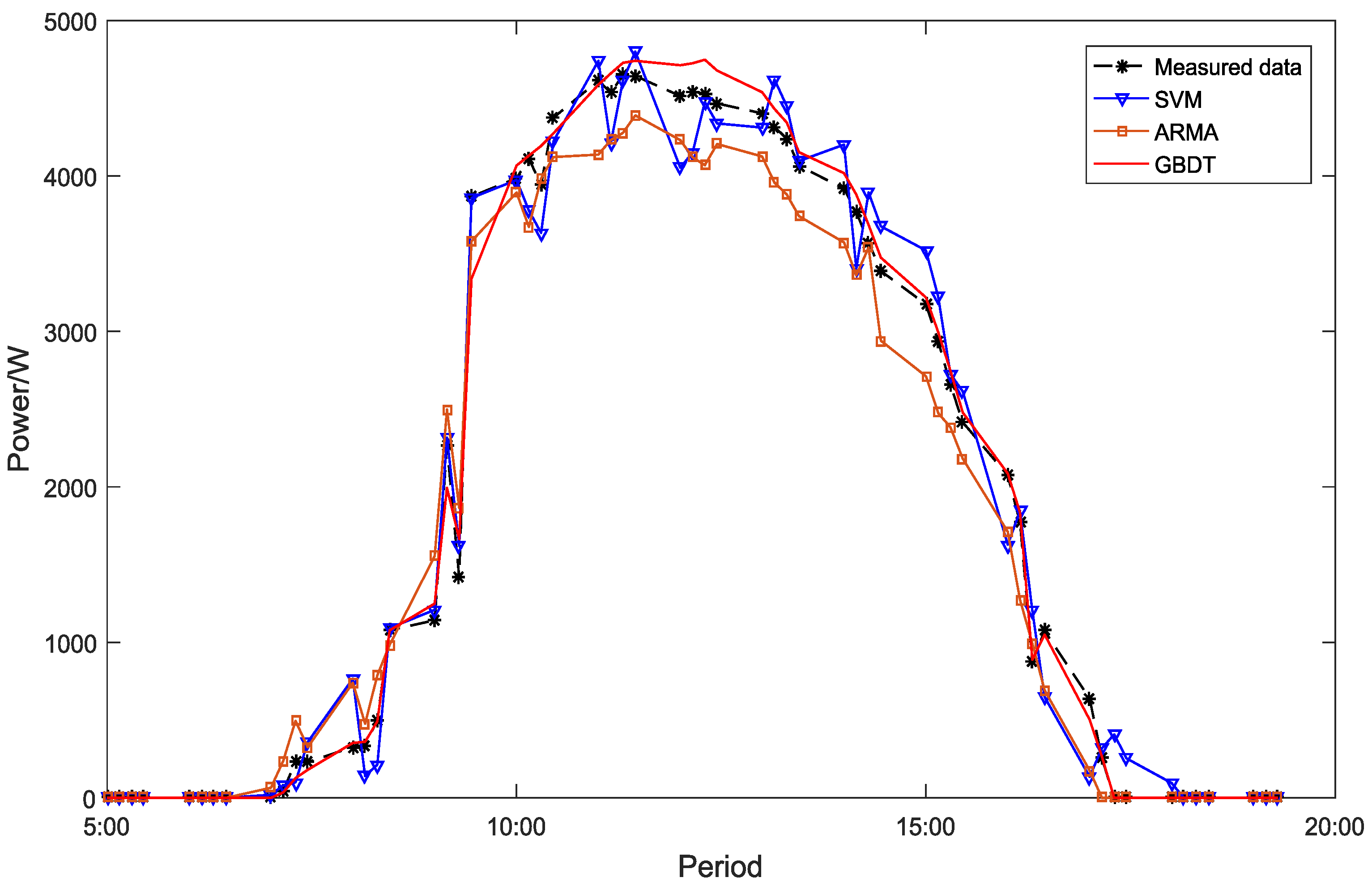
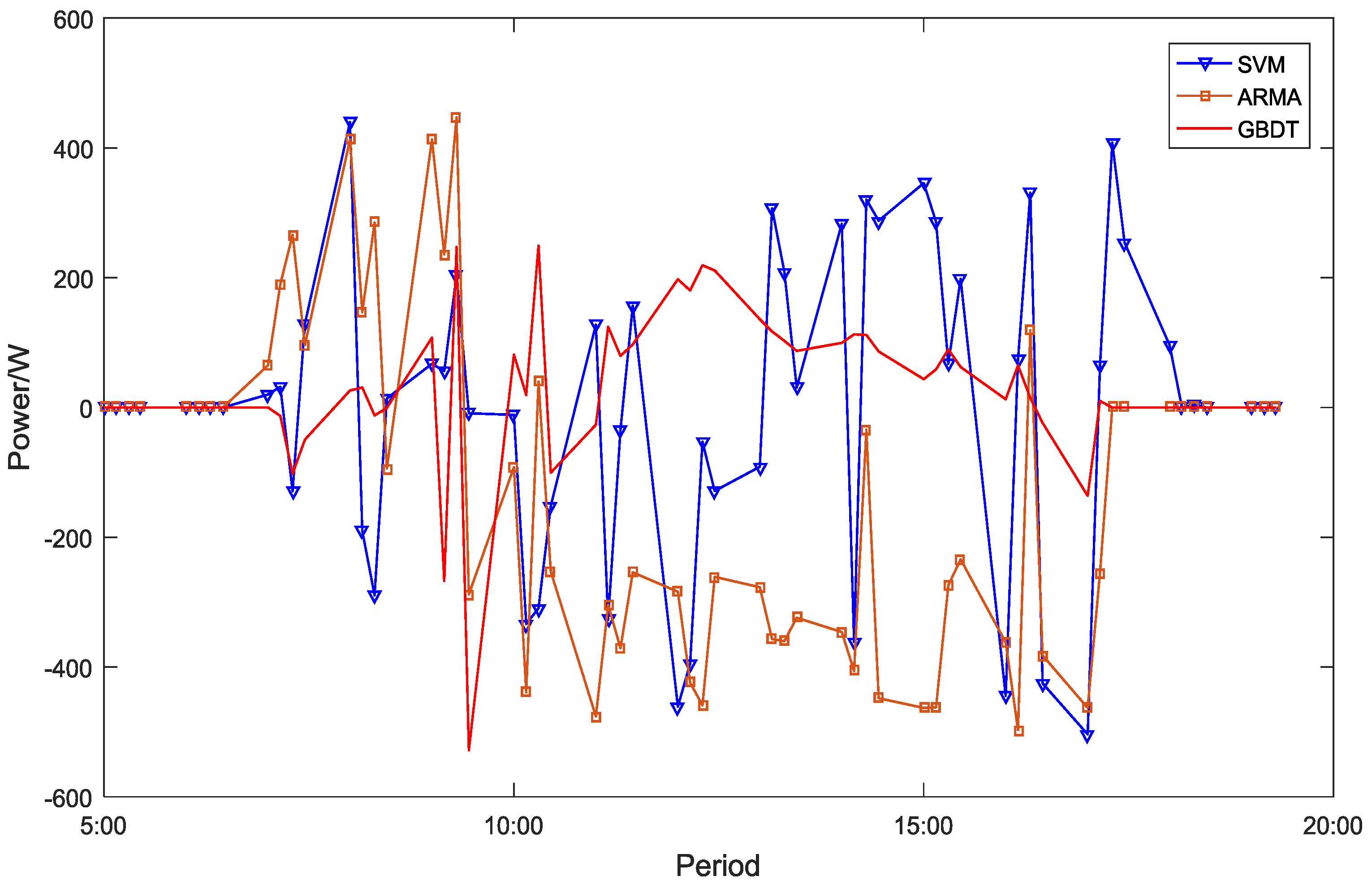
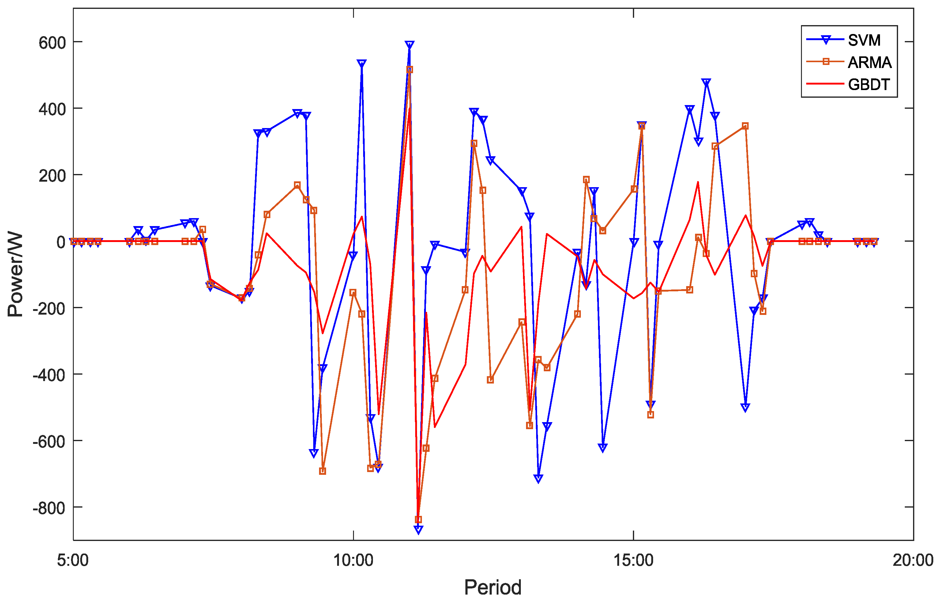
4.1. Accuracy Comparison in a Single Day

This paper compares the results of the two models on a certain sunny day (September 4) and rainy day (September 1) in 2015. The results including the predicted PV power data and actual data are shown in Figure 3, Figure 4, Figure 5 and Figure 6.
Figure 3 shows that the measured data of PV power, the output data of the prediction model based on the SVM algorithm, and the output data of the proposed prediction model based on the GBDT algorithm on September 4. The abscissa represents the predicted periods in one day and the ordinate represents the power value. As shown in Figure 3, the predictive stability of the GBDT model is higher than that of the SVM model and the ARMA model at the peak of the sunny PV output. The fluctuation range of the SVM model’s prediction curve is wide and that means the SVM model lacks deficiency in stability. The forecast accuracy of the ARMA model is also lower than that of the GBDT model, evidently.
The prediction errors of the two models at each moment are intuitively shown in Figure 4. The values are the differences between the predicted values and actual values. The prediction error curve of the prediction model based on the GBDT algorithm is smoother and stable most of the time.
Figure 5, Figure 6 show the measured data of PV power, the output data of the prediction model based on the SVM algorithm, and the output data of the proposed prediction model based on the GBDT algorithm on a rainy day on September 1. As we can see in Figure 5, Figure 6, the fluctuation of photovoltaic power generation on rainy days is more severe than that of the sunny day. Faced with such severe power fluctuations, the prediction stability of the GBDT model is still higher than that of the SVM model and ARMA model.
Comparing Figure 3 and Figure 5, as well as Figure 4 and Figure 6, it can be seen that the prediction accuracy of the prediction model based on the GBDT algorithm is more stable with respect to the SVM algorithm and ARMA algorithm. On the rainy day when the SVM and ARMA algorithm’s error is large, the proposed prediction model based on the GBDT algorithm can achieve better accuracy. In a word, the proposed prediction model based on the GBDT algorithm is effective and reliable.

4.2. Monthly Average Accuracy Comparison

The results based on the one-day data are to show the performance intuitively, but are not convincing enough due to the randomness existing in solar generation. In order to analyze the accuracy of the two algorithms further, we chose the data in April (spring), July (summer), October (autumn), and January (winter) for testing. The comparison results of nRMSE and MAPE are shown in Table 1.
As shown in Table 1, the prediction accuracies of the SVM algorithm and ARMA algorithm in different seasons are not as stable as that of the GBDT algorithm, especially for the accuracy measured in MAPE. The reason is that the prediction errors of the SVM algorithm and ARMA algorithm are large when the output power is small. On the contrary, the discrete piecewise function of the GBDT algorithm can fit well the non-continuous function relations, so it can avoid this kind of problem, resulting in more stable performance in different power conditions.

5. Conclusions

In this paper, the GBDT integrated algorithm was used to solve the problem of PV power prediction. In essence, the GBDT algorithm integrates weak learners with binary fissions by using the integrated algorithm of gradient descent. The decision tree algorithm is able to adjust its structure according to the data characteristics, and hence it is able to fit well the relationship of non-continuous functions and is suitable for the scenario of PV power prediction. The GBDT algorithm, as an integrated algorithm, inherits the advantages of the decision tree algorithm. At the same time, it can effectively avoid the over-fitting problem compared with a single decision tree algorithm.
The case studies show that the proposed model based on the GBDT algorithm can fit well the relationship between PV power and input variables and avoid the over-fitting problem. Compared with the SVM-based PV model, the proposed PV prediction model based on the GBDT algorithm is relatively stable no matter whether on a single (sunny or rainy) day or in different seasons. Once the model has been trained, the prediction calculation is relatively simple, and good prediction results can be obtained.

Author Contributions

J.W. contributed to model establishing and paper writing. Many ideas on the paper are suggested by P.L. to support the work, and P.L. did the job of performing the simulations. R.R. and Y.Z. analyzed the data. Y.C. reviewed the work and modified the paper. In general, all authors cooperated as much as possible during all progress of the research.

Acknowledgments

This work was supported by the National Natural Science Foundation of China (NSFC) (51477111) and the National Key Research and Development Program of China (2016YFB0901102).

Conflicts of Interest

The authors declare no conflict of interest.

References

  1. Available, N. 2010 Solar Technologies Market Report; Office of Scientific & Technical Information Technical Reports; Energy Efficiency and Renewable Energy: Washington, DC, USA, 2011. [Google Scholar]
  2. Babaa, S.E.; Armstrong, M.; Pickert, V. Overview of Maximum Power Point Tracking Control Methods for PV Systems. J. Power Energy Eng. 2014, 2, 59–72. [Google Scholar] [CrossRef]
  3. Kouro, S.; Leon, J.I.; Vinnikov, D.; Franquelo, L.G. Grid-Connected Photovoltaic Systems: An Overview of Recent Research and Emerging PV Converter Technology. IEEE Ind. Electron. Mag. 2015, 9, 47–61. [Google Scholar] [CrossRef]
  4. Solangi, K.H.; Islam, M.R.; Saidur, R.; Rahim, N.A.; Fayaz, H. A Review on Global Solar Energy Policy. Renew. Sustain. Energy Rev. 2011, 15, 2149–2163. [Google Scholar] [CrossRef]
  5. Paatero, J.V.; Lund, P.D. Effects of Large-Scale Photovoltaic Power Integration on Electricity Distribution Networks. Renew. Energy 2007, 32, 216–234. [Google Scholar] [CrossRef]
  6. Aydinalp-Koksal, M.; Ugursal, V.I. Comparison of Neural Network, Conditional Demand Analysis, and Engineering Approaches for Modeling End-use Energy Consumption in the Residential Sector. Appl. Energy 2008, 85, 271–296. [Google Scholar] [CrossRef]
  7. Wu, Z.; Tazvinga, H.; Xia, X. Demand Side Management of Photovoltaic-battery Hybrid System. Appl. Energy 2015, 148, 294–304. [Google Scholar] [CrossRef]
  8. Ke, B.R.; Ku, T.T.; Ke, Y.L.; Chuang, C.Y.; Chen, H.Z. Sizing the Battery Energy Storage System on a University Campus With Prediction of Load and Photovoltaic Generation. IEEE Trans. Ind. Appl. 2016, 52, 1136–1147. [Google Scholar]
  9. Elminir, H.K.; Azzam, Y.A.; Younes, F.I. Prediction of Hourly and Daily Diffuse Fraction Using Neural Network, as Compared to Linear Regression Models. Energy 2007, 32, 1513–1523. [Google Scholar] [CrossRef]
  10. Voyant, C.; Notton, G.; Kalogirou, S.; Nivet, M.L.; Paoli, C.; Motte, F.; Fouilloy, A. Machine Learning methods for solar radiation forecasting: A review. Renew. Energy 2017, 105, 569–582. [Google Scholar] [CrossRef]
  11. Zhu, H.; Li, X.; Sun, Q.; Nie, L.; Yao, J.; Zhao, G. A Power Prediction Method for Photovoltaic Power Plant Based on Wavelet Decomposition and Artificial Neural Networks. Energies 2016, 9, 11. [Google Scholar] [CrossRef]
  12. Mellit, A.; Pavan, A.M.; Lughi, V. Short-term Forecasting of Power Production in a Large-scale Photovoltaic Plant. Solar Energy 2014, 105, 401–413. [Google Scholar] [CrossRef]
  13. Yao, Z.; Fei, P.; Shen, Y. Short-term Prediction of Photovoltaic Power Generation Output Based on GA-BP and POS-BP Neural Network. Power Syst. Prot. Control 2015, 43, 83–89. [Google Scholar]
  14. Shi, J.; Lee, W.J.; Liu, Y.; Yang, Y.; Wang, P. Forecasting Power Output of Photovoltaic Systems Based on Weather Classification and Support Vector Machines. IEEE Trans. Ind. Appl. 2012, 48, 1064–1069. [Google Scholar] [CrossRef]
  15. Wang, J.; Ran, R.; Song, Z.; Sun, J. Short-Term Photovoltaic Power Generation Forecasting Based on Environmental Factors and GA-SVM. J. Electr. Eng. Technol. 2017, 12, 64–71. [Google Scholar] [CrossRef]
  16. Malvoni, M.; Giorgi, M.G.D.; Congedo, P.M. Photovoltaic Forecast Based on Hybrid PCA-LSSVM Using Dimensionality Reducted Data. Neurocomputing 2016, 211, 72–83. [Google Scholar] [CrossRef]
  17. Yang, H.T.; Huang, C.M.; Huang, Y.C.; Pai, Y.S. A Weather-Based Hybrid Method for 1-Day Ahead Hourly Forecasting of PV Power Output. IEEE Trans. Sustain. Energy 2014, 5, 917–926. [Google Scholar] [CrossRef]
  18. Gala, Y.; Fernández, Á.; Díaz, J.; Dorronsoro, J.R. Hybrid machine learning forecasting of solar radiation values. Neurocomputing 2016, 176, 48–59. [Google Scholar] [CrossRef]
  19. Chaouachi, A.; Kamel, R.M.; Nagasaka, K. Neural Network Ensemble-Based Solar Power Generation Short-Term Forecasting. J. Adv. Comput. Intell. Intell. Inform. 2011, 14, 69–75. [Google Scholar] [CrossRef]
  20. Mohammed, A.A.; Aung, Z. Ensemble Learning Approach for Probabilistic Forecasting of Solar Power Generation. Energies 2016, 9, 1017. [Google Scholar] [CrossRef]
  21. Friedman, J.H. Stochastic Gradient Boosting. Comput. Stat. Data Anal. 2002, 38, 367–378. [Google Scholar] [CrossRef]
  22. Duffy, N.; Helmbold, D. Boosting Methods for Regression. Mach. Learn. 2002, 47, 153–200. [Google Scholar] [CrossRef]
  23. Natekin, A.; Knoll, A. Gradient Boosting Machines, a Tutorial. Front. Neurorobot. 2013, 7, 21. [Google Scholar] [CrossRef] [PubMed]
  24. Breiman, L.; Friedman, J.H.; Olshen, R.A. CART: Classification and Regression Trees. Biometrics 1984, 40, 358–380. [Google Scholar]
  25. Sakar, A.; Mammone, R.J. Growing and Pruning Neural Tree Networks. IEEE Trans. Comput. 1993, 42, 291–299. [Google Scholar] [CrossRef]
  26. Friedman, J.H. Greedy function approximation: A gradient boosting machine. Ann. Stat. 2001, 29, 1189–1232. [Google Scholar] [CrossRef]
  27. Riffonneau, Y.; Bacha, S.; Barruel, F.; Ploix, S. Optimal Power Flow Management for Grid Connected PV Systems with Batteries. IEEE Trans. Sustain. Energy 2011, 2, 309–320. [Google Scholar] [CrossRef]
  28. University of Oregon Solar Radiation Monitoring Laboratory [EB/OL]. Available online: http://solardat.uoregon.edu/SelectDailyTotal.html (accessed on 9 May 2016).
Figure 1. The flowchart of photovoltaic prediction model based on the Gradient Boost Decision Tree (GBDT).
Applsci 08 00689 g001
Figure 2. The statistical data of the solar power plant in Ashland in 2015.
Applsci 08 00689 g002
Figure 3. Comparison of model prediction accuracy on sunny day.
Applsci 08 00689 g003
Figure 4. Comparison of model prediction errors on sunny day.
Applsci 08 00689 g004
Figure 5. Comparison of model prediction accuracy on rainy day.
Applsci 08 00689 g005
Figure 6. Comparison of model prediction errors on rainy day.
Applsci 08 00689 g006
Table 1. Comparison of prediction accuracy monthly.
SeasonModelnRMSEMAPE
April (spring)GBDT0.07190.1420
SVM0.10720.1783
ARMA0.11430.1867
July (summer)GBDT0.07720.1365
SVM0.09570.1541
ARMA0.11060.1618
October (autumn)GBDT0.07030.1477
SVM0.11080.1732
ARMA0.12290.1894
January (winter)GBDT0.06960.15270.1876
SVM0.0985
ARMA0.11210.2013

