An Effective Directional Residual Interpolation Algorithm for Color Image Demosaicking

Abstract

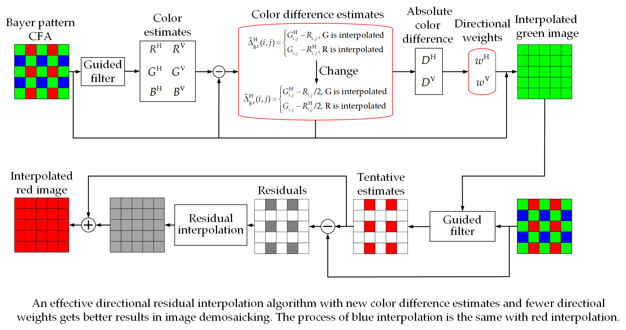
In this paper, we propose an effective directional Bayer color filter array (CFA) demosaicking algorithm based on residual interpolation (RI). The proposed directional interpolation algorithm aims to reduce computational complexity and get more accurate interpolated pixel values in the complex edge areas. We use the horizontal and vertical weights to combine and smooth color difference estimations. Compared with four directional weights in minimized Laplacian residual interpolation, the proposed algorithm not only guarantees the quality of color images but also reduces the computational complexity. Generally, the directional estimations may be inaccurately calculated because of the false edge information in irregular edges. We alleviate it by using a new method to calculate the directional color difference estimations. Experimental results show that the proposed algorithm provides outstanding performance compared with some previous algorithms, especially in the complex edge areas. In addition, it has lower computational complexity and better visual effect.

1. Introduction

In recent years, many more people choose digital cameras to take pictures. Each digital color image needs at least three color samples at each pixel. To achieve the requirement, cameras have to set three sensors to get red (R), green (G), and blue (B) components at each pixel. However, in view of equipment costs, there is only one signal sensor set at each pixel. The sensors compose a color filter array (CFA). The CFA needs only one color to be observed and the other two missing colors can be estimated at each pixel. The process of estimation is called demosaicking [1]. The method effectively reduces the density of the sensors.

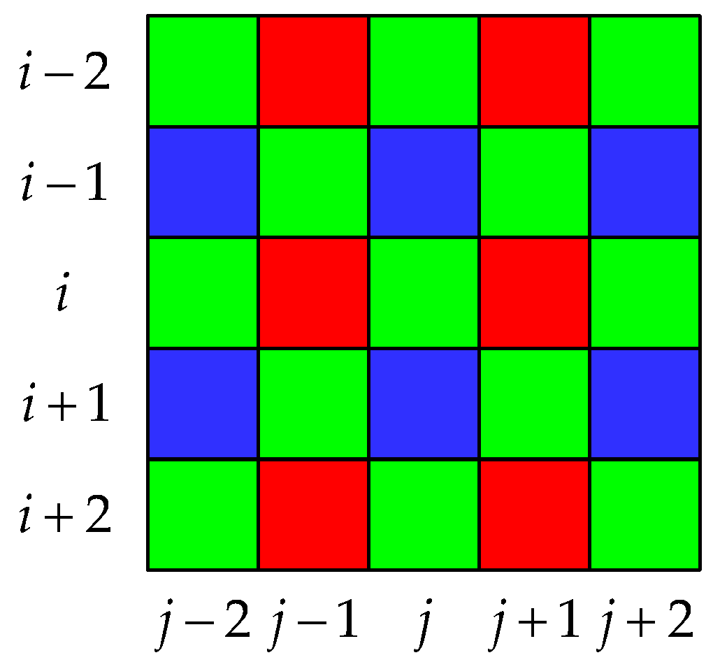
Bayer pattern CFA [2] is the most common pattern for CFA, as shown in Figure 1. The G pixels are estimated on a quincunx grid, while R or B pixels are estimated on a rectangular grid in Bayer pattern CFA. The density of G pixels is as twice as that of R or that of B in Bayer pattern CFA, because the peak sensitivity of human visual system (HVS) lies in the wavelength of G light.

For the original Bayer pattern CFA, the commonly used demosaicking algorithms include the nearest neighbor interpolation [3], bilinear interpolation [4], and bicubic interpolation [5]. These demosaicking algorithms generate the other two missing colors at each pixel with linear averaging color pixel values. They can be widely applied in a real-time system because of the lower computational complexity. However, they have significant zipper artifacts around line edges in demosaicking images.

To solve this problem, several demosaicking algorithms [6,7,8] have been proposed. Malvar [6] proposed a high-quality linear interpolation algorithm for CFA demosaicking. It presents a simple linear demosaicking filter that has better performance and lower computational complexity. Many previous demosaicking algorithms are based on inter-channel color difference interpolation. For instance, Yu [7] proposed a novel demosaicking algorithm exploiting joint intra-channel color correlation and inter-channel color difference, but it does not perform well enough when images have sharp color transition areas. Normally, G pixel values are first interpolated in most Bayer pattern CFA demosaicking algorithms, since the density of G pixel is as twice as that of R or that of B. On the contrary, Zhang et al. [8] proposed a novel demosaicking algorithm that estimated two independent chrominance components (R and B). Then they estimated the luminance component (G). As a result, the demosaicking algorithm can avoid the associated estimation error.

Although the above mentioned nonadaptive algorithms [6,7,8] have lower computational complexity for the CFA, most of them perform color directional interpolation based on the estimated gradient. However, the gradient estimations of the methods may not be robust in texture areas and edges. Based on the directional linear minimum mean square-error estimation (DLMMSE) framework, Zhang and Wu [9] proposed an adaptive algorithm to improve the problem. They assumed that the primary difference signals between G and R or G and B channels are low-pass. In both horizontal and vertical directions, the missing G pixel values are adaptively estimated by DLMMSE. Some demosaicking algorithms provide novel contributions such as square-on-point neighborhood and lattice variables [10]. In [10], a corrective term and localized polling were used to improve the performance of the reconstructed images. However, the corrective term is empirically derived. Shi et al. [11] demonstrated that the input image is divided into two different area types and each type adopts different interpolation respectively. In edge areas, they recovered edge information with weights by using multidirectional components. The demosaicking algorithm has the advantages of region adaptation. Chen and Chang [12] detected edge characteristics by comparing color difference in horizontal and vertical directions. Then they used different weighted interpolation to effectively reduce the color artifacts at the edge of the image and enhance the image quality. Pekkucuksen and Altunbasak [13] exploited an orientation-free edge strength filter to estimate edge information, and applied it to reconstruction process. However, the demosaicking algorithm failed in utilizing spectral correlation.

To solve this problem, Tsai and Song [14] proposed a novel edge-adaptive demosaicking algorithm, which reduces the aliasing error in R and B channels by exploiting high-frequency information of the G channel. Adams and Hamilton [15] exploited chrominance and luminance with 5 × 5 neighborhoods interpolation equation. The advantage of method is computationally efficient in both execution time and memory storage requirements. On the basis of this interpolation method, several demosaicking algorithms [16,17,18] have been proposed. Pekkucuksen and Altunbasak [16] designed a gradient-based threshold free color filter. It combined the estimations of color difference from each direction into a gradient without setting the thresholds. To estimate different directions, in [17], the color differences were combined by using multiscale color gradients adaptively. This algorithm does not need any threshold because it makes no hard decision. Chen et al. [18] proposed an algorithm by combining voting-based edge direction detection with weighting-based interpolation, because some other algorithms may use false edge information in irregular edges.

The residual interpolation (RI) method has been widely used recently [19,20,21,22,23,24,25]. The RI algorithm exploited the characteristics of the guided filter [26] and showed outstanding performance [19]. Kiku et al. [20] incorporated the RI into the gradient-based threshold free algorithm. The better the interpolation results of images are, the smaller the Laplacian energies of images will have. In this way, the RI algorithm combined with minimizing the Laplacian energies of the residuals, which is termed as minimized Laplacian RI (MLRI) [21]. Ye and Ma [22] exploited iterative RI process and reconstructed a highly accurate G channel to reduce reconstruction error for the first time. Wang and Jeon [23] reconstructed only R and B channels by using RI algorithm, while the missing color components of G channel were estimated by eight-direction weighted color difference interpolation. The demosaicking algorithm effectively combined the advantages of color difference interpolation and residual interpolation. Kim and Jeong [24] proposed a four-directional RI algorithm to reduce severe demosaicking artifacts. The adaptive residual interpolation (ARI) algorithm [25] adaptively combined two RI-based algorithms and selected the appropriate number of iterations at each pixel to improve the existing RI-based algorithm. However, the weakness of this algorithm is that the algorithm has high computational complexity.

Furthermore, a demosaicking algorithm was proposed for the multispectral filter array about RI in [27]. There are some demosaicking algorithms based on other patterns such as RGB-white color filter arrays [28]. The image reconstructed in [28] contains much important information that cannot be perceived in the color image reconstructed by conventional CFA. However, they still have other artifacts, and further improvements are needed.

RI can be used as an alternative to the widely used color different interpolation and it performs better in some image datasets. MLRI has better interpolation results because the images have smaller Laplacian energies. Furthermore, MLRI also produces other artifacts in some complex edge areas. However, we find that the directional color difference estimations are not completely the same as the actual values sometimes. With the process of research, we think the problem can be solved by reducing the weights of directional color difference estimations. This paper proposes an effective directional residual interpolation algorithm for color image demosaicking based on MLRI. We use the two weights, horizontal and vertical weights, while there are four directional weights in MLRI. In this way, our method reduces the computational complexity. Afterwards, we use a novel method to calculate the directional color difference estimations, and to combine and smooth the color difference estimations. The proposed algorithm can effectively reduce the influence of false edge information in irregular edges. In the following experiments, our proposed algorithm outperforms previous algorithms and provides better color fidelity.

The rest of this paper is organized as follows. Section 2 starts with a brief of MLRI and related work. The proposed method is described in Section 3. Experimental results of the proposed method are presented in Section 4. Conclusions and remarks on possible future work are given in Section 5.

2. Related Work

2.1. The Outline of MLRI

The proposed algorithm is based on MLRI. First, we introduce the outline of MLRI. The interpolation process of the G pixel can be divided into three steps in MLRI.

Step 1.

The G pixel values are calculated through residuals at the location of R and B pixels from horizontal and vertical directions. R and B pixel values also are calculated at the location of G pixels. The calculation of the residuals replaces the calculation of the color difference in Adams and Hamilton’s interpolation equation [15].

Step 2.

MLRI calculates both horizontal and vertical color difference estimations based on Step 1 at each pixel, then MLRI combines and smooths the color difference estimations.

Step 3.

The color difference estimations are added to the observed R or B pixel values. It aims to interpolate G pixel values.

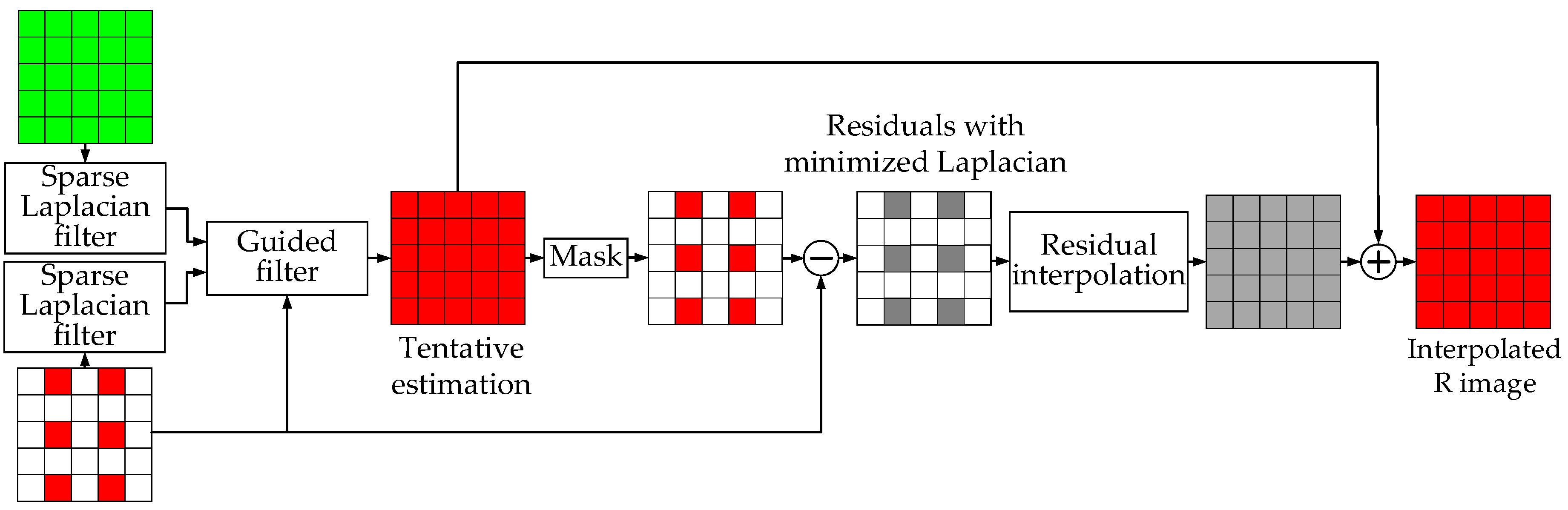
After interpolating the G pixel, MLRI interpolates the R and B pixel values, and the method simply replaces the traditional method of using color difference as shown in Figure 2.

In the past decades, color difference interpolation has been used gradually in image demosaicking. However, residual interpolation has been used recently in MLRI. MLRI uses a novel filter called guided filter. We compare the process of MLRI with that of the color difference interpolation in calculating R pixel. The process of calculating B pixel is similar.

We introduce the process of color difference interpolation to help us understand the process of MLRI. Firstly, the missing pixel in G image is the average of four observed G pixels around it. By this way, it can get G pixel values at each pixel to combine the interpolated G image. Secondly, the color differences between R and G are calculated at the locations of R pixel by subtracting the interpolated G pixel values from the observed R pixel values ($R-G$). Then color differences are interpolated. Finally, an interpolated R image can be calculated by adding G pixel values to the interpolated color image.

Figure 2 shows the interpolation of the R pixel values by using MLRI in detail according to [21]. First, it can get the interpolated G image as the same method as the color difference interpolation. To minimize the Laplacian energies of the residuals, the guided image and the input image are first passed through a sparse Laplacian filter. The sparse Laplacian filter with MLRI is shown in

Table 1. The sparse Laplacian filter used in MLRI.

Direction	G Channel Interpolation	R and B Channels Interpolation
Horizontal	$(\begin{array}{rrrrr}\hfill 1& \hfill 0& \hfill -2& \hfill 0& \hfill 1\end{array})$	$\left(\begin{array}{ccccc}0& 0& 1& 0& 0\\ 0& 0& 0& 0& 0\\ 1& 0& -4& 0& 1\\ 0& 0& 0& 0& 0\\ 0& 0& 1& 0& 0\end{array}\right)$
Vertical	$\left(\begin{array}{c}1\\ 0\\ -2\\ 0\\ 1\end{array}\right)$

. Then MLRI uses the guided filter to generate the tentative estimation of the R ($\stackrel{⌣}{R}$) image. The interpolated G image is used as the guided image, and the observed R image is used as the input image. After that, tentative estimation of the R image uses a mask to obtain the value at the location of R image. Then minimized Laplacian residuals are calculated at the location of R pixel by subtracting the tentative estimation ${\stackrel{⌣}{R}}^{\mathrm{H}}$ values from the observed R pixel values ($R-\stackrel{⌣}{R}$). Then MLRI interpolates the residuals. Finally, an interpolated R image can be calculated by adding the $\stackrel{⌣}{R}$ image to the interpolated residual image.

2.2. Guided Filter

As an example, we describe how to get the $\stackrel{⌣}{R}$ image by the guided filter in detail. The guided filter can accurately transfer the structures of the guided image to the filtered output. It has a good performance in edge-preserving smoothing and does not suffer from reversal artifacts. Thus, it can be used in demosaicking area. Furthermore, the guided filter also can be applied in denoising, edge-preserving, dehazing, and guided feathering.

The interpolated G image can be regarded as a guided image, and the observed R image can be regarded as an input image. To minimize the Laplacian energies of the residuals, the guided image and the input image are first passed through a sparse Laplacian filter. After that, the guided image uses a mask to obtain the value at the location of input image.

The guided filter assumption is a local linear model between the guided image $I$ and the filtering output $q$ in a window as shown in Equation (1):

$$q_i=a_k{I}_i+b_k,\forall i\in w_k,$$

(1)

where $i$ is the pixel in $w_k$, and $w_k$ is a window centered at the pixel $k$; $(a_k,b_k)$, which are assumed to be constant, are linear coefficients in $w_k$. To determine the linear coefficients $(a_k,b_k)$, the cost function is given as:

$$E(a_k,b_k)={{\displaystyle \sum _{i\in w_k}(a_k{I}_i+b_k-p_i)}}^2,$$

(2)

where $p_i$ is a pixel at $w_k$ in the input image. To minimize Equation (2), the solution is given by:

$$a_k=\frac{\frac{1}{\left|w\right|}{\displaystyle \sum _{i\in w_k}{I}_i-{\mu }_k{\overline{p}}_k}}{{\sigma }_k^2},$$

(3)

$$b_k={\overline{p}}_k-a_k{\mu }_k,$$

(4)

where ${\mu }_k$ and ${\sigma }_k^2$ are the mean and variance of $I$ in $w_k$, $\left|w\right|$ is the number of pixels in $w_k$, and ${\overline{p}}_k=\frac{1}{\left|w\right|}{\displaystyle \sum _{i\in w_k}{p}_i}$ is the mean of $p$ in $w_k$. However, a pixel $i$ is involved in all the overlapping windows $w_k$ that covers $i$. The value of $q_i$ in Equation (1) is not identical when it is computed in different windows, so we rewrite Equation (1) by:

$$q_i={\overline{a}}_i{I}_i+{\overline{b}}_i,$$

(5)

where ${\overline{a}}_i=\frac{{\displaystyle \sum _{k\in w_i}{a}_k}}{\left|w\right|}$ and ${\overline{b}}_i=\frac{{\displaystyle \sum _{k\in w_i}{b}_k}}{\left|w\right|}$ are the average coefficients of all windows overlapping $i$.

3. The Proposed Demosaicking Algorithm

Our proposed demosaicking algorithm, which is a high-performance algorithm, is based on MLRI. We designed a new method that could effectively calculate the horizontal and vertical weights. It can also combine and smooth the horizontal and vertical color difference estimations. It improves the visual effect of the complex texture region. Compared with four directional weights in MLRI, the amount of calculation in the proposed demosaicking algorithm is efficiently reduced.

It is vital to interpolate the missing G pixel values because the peak sensitivity in HVS lies in the wavelength of the green light. Since the missing G pixel values are the key to the performance of the proposed algorithm, we first estimate the G pixel values at each pixel. Then we estimate the R and B pixel values, which are based on the interpolated G pixel values.

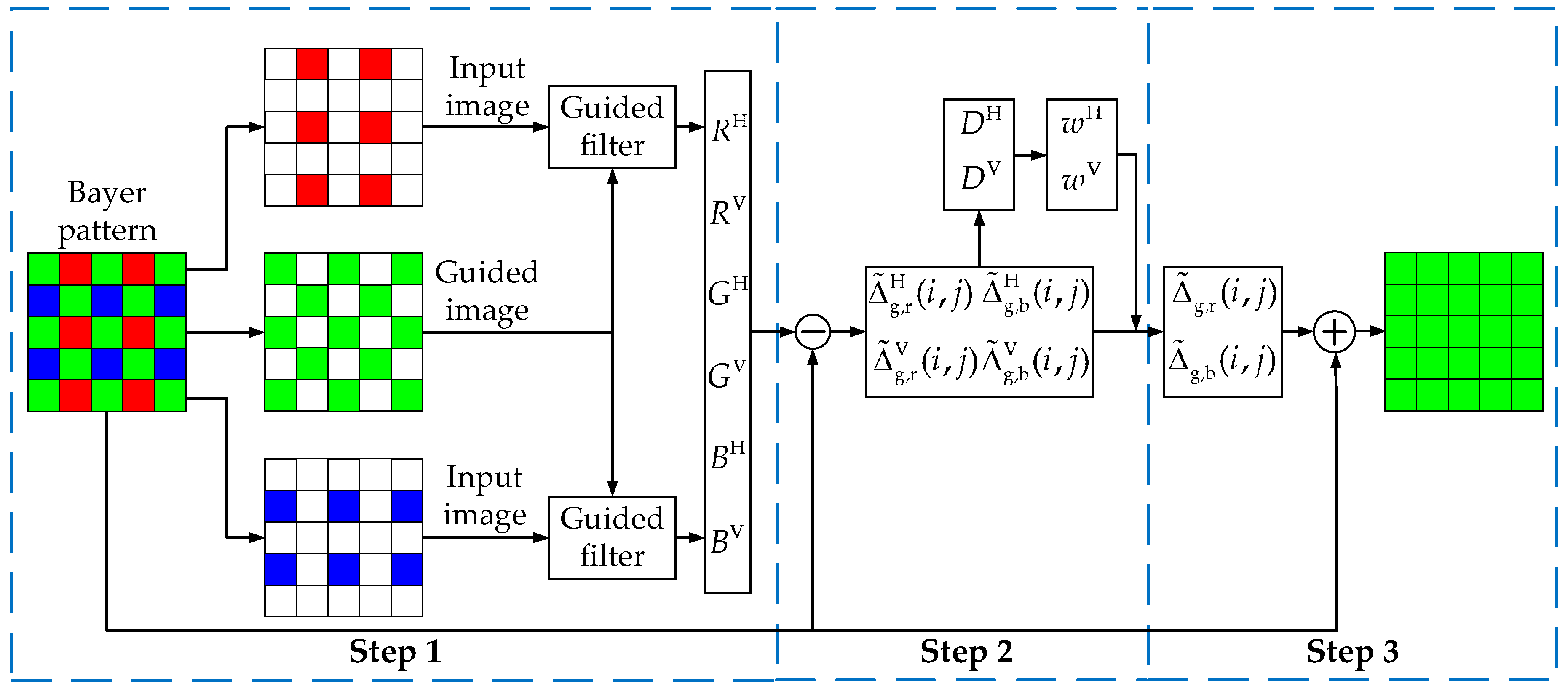
Similarly, compared with MLRI, the interpolation processes of the missing G pixel values can be divided into three steps in the same way as that in MLRI [21].

Step 1.

The linear color difference interpolation in Adams and Hamilton’s interpolation equation [15] can be replaced by MLRI [21]. Then the new equation estimates the G, R, and B pixels in horizontal and vertical directions, so we can get $G^{\mathrm{H}}$, $G^{\mathrm{V}}$, $R^{\mathrm{H}}$, $R^{\mathrm{V}}$, $B^{\mathrm{H}}$, and $B^{\mathrm{V}}$.

Step 2.

The horizontal and vertical color difference estimations are calculated, and we can generate the horizontal and vertical weights at each pixel.

Step 3.

To get color difference, the horizontal and vertical color difference estimations are combined and smoothed by two directional weights. As a result, the G pixel values at the location of R and B pixels are generated by adding final color difference to the observed R or B pixel values.

To sum up, the outline of the interpolation processes of the missing G pixel values is shown in Figure 3.

3.1. The Calculation Process of Directionaly Estimated Pixel Value

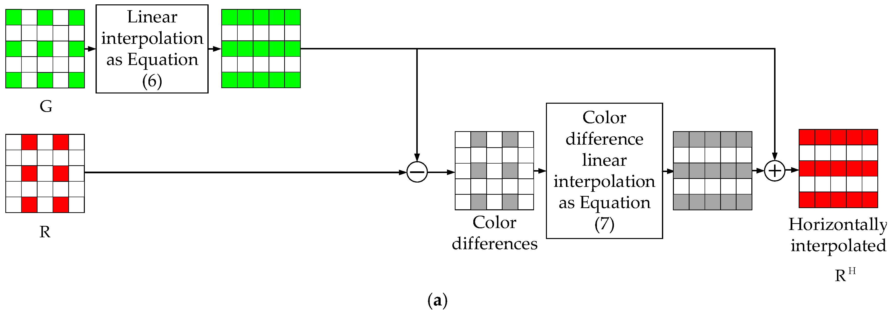
In Step 1, the Adams and Hamilton’s interpolation equation [15] can be considered as a linear model, as shown in Figure 4a. The linear color model can be replaced by MLRI [21]. The locations of R and B are symmetrical and the amount of R pixels and B pixels are same. To simplify the explanation, we explain the estimation of the R pixel values in the horizontal direction in detail, as shown in Figure 4b.

The linear model in Adams and Hamilton’s interpolation equation can be expressed as:

$$R_{i,j}^{\mathrm{H}}=(R_{i,j-1}+R_{i,j+1})/2+(2\times G_{i,j}-G_{i,j-2}-G_{i,j+2})/4,$$

(6)

where $R^{\mathrm{H}}$ is the horizontally estimated R pixel value, the suffix $(i,j)$ represents the target pixel coordinates. This interpolation equation can be considered the linear interpolation, which is shown in Equation (7):

$$R_{i,j}^{\mathrm{H}}-G_{i,j}=(R_{i,j-1}-G_{i,j-1}^{\mathrm{H}})/2+(R_{i,j+1}-G_{i,j+1}^{\mathrm{H}})/2.$$

(7)

Here $G^{\mathrm{H}}$ is the G pixel value horizontally estimated at the R pixel and $G^{\mathrm{H}}$ is calculated as follows:

$$G_{i,j-1}^{\mathrm{H}}=(G_{i,j-2}+G_{i,j})/2,$$

(8)

$$G_{i,j+1}^{\mathrm{H}}=(G_{i,j}+G_{i,j+2})/2.$$

(9)

Similarly, we can calculate $G^{\mathrm{H}}$ and $G^{\mathrm{V}}$ at the R and B pixels. MLRI uses the tentative estimations to replace of these estimated G pixel values as shown in Figure 4b. As a result, Equation (6) can be rewritten as:

$$R_{i,j}^{\mathrm{H}}-{\stackrel{⌣}{R}}_{i,j}^{\mathrm{H}}=(R_{i,j-1}-{\stackrel{⌣}{R}}_{i,j-1}^{\mathrm{H}})/2+(R_{i,j+1}-{\stackrel{⌣}{R}}_{i,j+1}^{\mathrm{H}})/2,$$

(10)

where ${\stackrel{⌣}{R}}^{\mathrm{H}}$ is the tentative estimated R image.

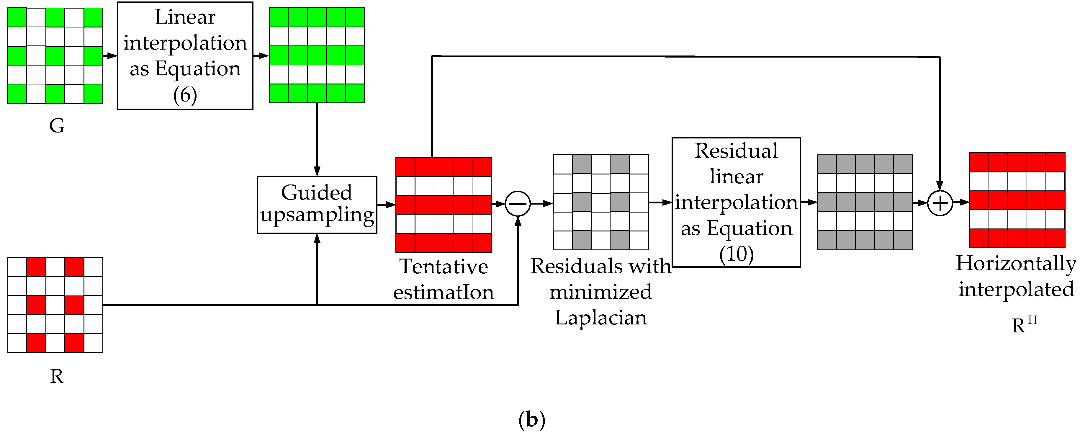
To sum up, the horizontally estimated G pixel value at the location of R pixel can be calculated by Equations (8) and (9) at first. Then the interpolated $G^{\mathrm{H}}$ image is used as the guided image. As a result, the tentative estimation ${\stackrel{⌣}{R}}^{\mathrm{H}}$ is generated by guided filter. The residual can be calculated after subtracting the tentative estimation ${\stackrel{⌣}{R}}^{\mathrm{H}}$ value from the observed R pixel values. After that, residuals are interpolated by Equation (10) at each pixel. We use the residuals to add the tentative estimation ${\stackrel{⌣}{R}}^{\mathrm{H}}$ and generate the horizontally estimated R pixel value $R^{\mathrm{H}}$.

$R^{\mathrm{V}}$, $B^{\mathrm{H}}$, and $B^{\mathrm{V}}$ at G pixel can be similarly generated by Step 1.

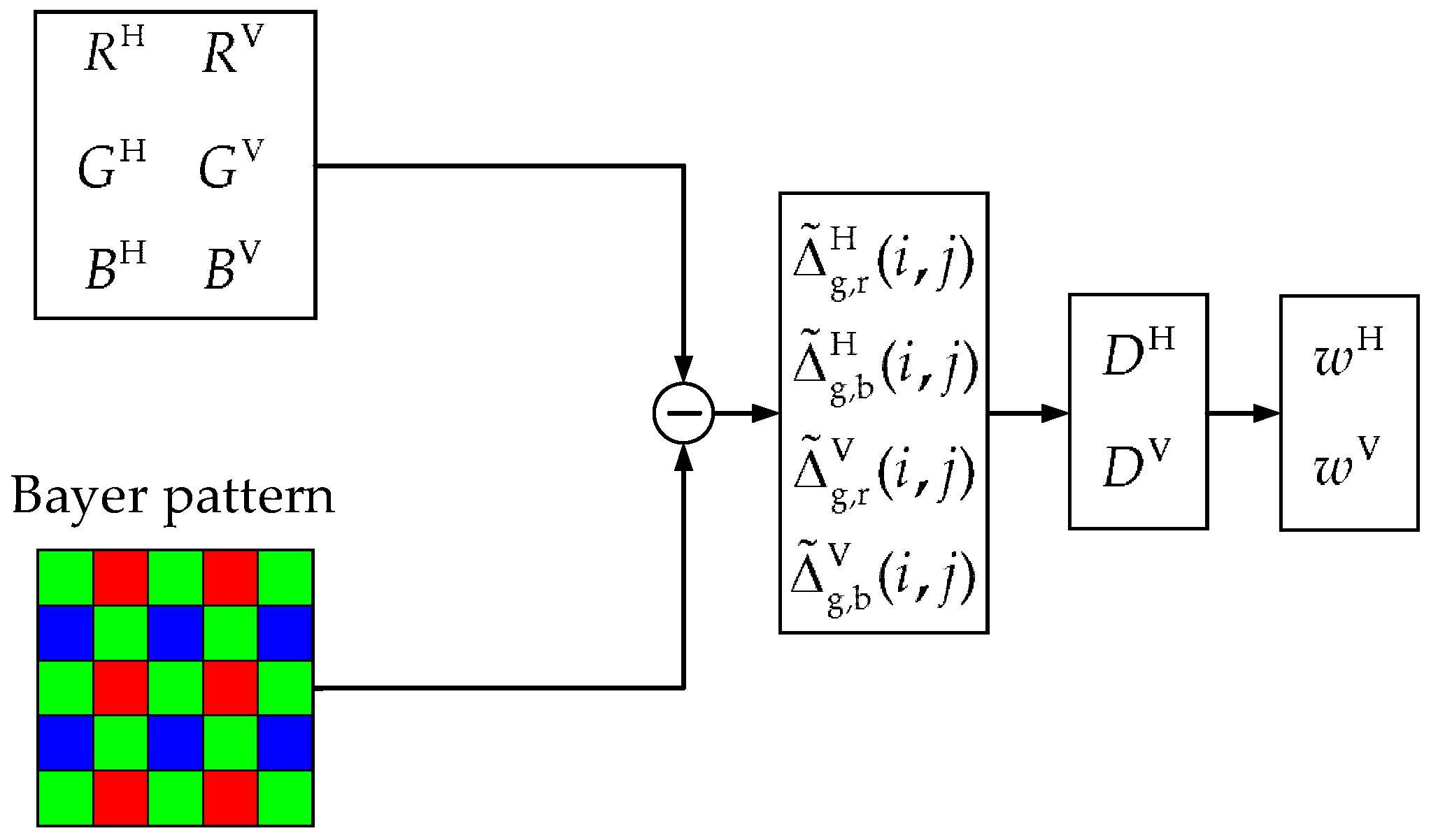
3.2. The Calculation Process of Directional Weights

We can get an observed pixel value and two directionally estimated values at each pixel after Step 1. In this section, we use the directional color difference estimations and the absolute color difference gradients to calculate the directional weights. The process is shown in Figure 5.

The directional color difference estimations can be calculated by Equation (11) in MLRI.

$${\tilde{\Delta }}_{\mathrm{g},\mathrm{r}}^{\mathrm{H}}(i,j)=\{\begin{array}{l}{G}_{i,j}^{\mathrm{H}}-R_{i,j},\mathrm{G}\mathrm{is}\mathrm{interpolated}\\ G_{i,j}-R_{i,j}^{\mathrm{H}},\mathrm{R}\mathrm{is}\mathrm{interpolated}\end{array},{\tilde{\Delta }}_{\mathrm{g},\mathrm{r}}^{\mathrm{V}}(i,j)=\{\begin{array}{l}{G}_{i,j}^{\mathrm{V}}-R_{i,j},\mathrm{G}\mathrm{is}\mathrm{interpolated}\\ G_{i,j}-R_{i,j}^{\mathrm{V}},\mathrm{R}\mathrm{is}\mathrm{interpolated}\end{array},$$

(11)

where ${\tilde{\Delta }}_{\mathrm{g},\mathrm{r}}^{\mathrm{H}}$ is the horizontal color difference estimation between G and R image, and ${\tilde{\Delta }}_{\mathrm{g},\mathrm{r}}^{\mathrm{V}}$ is the vertical color difference estimation between G and R image. The effective combination of the directional color difference estimations is the most important factor of a successful algorithm. However, the horizontally estimated R pixel value $R^{\mathrm{H}}$ in Equation (11) is not completely the same as the actual value. There are differences between the missing actual value during imaging and the reconstructed value. To reduce the influence of differences and to get estimated values, we reduce the weight of $R^{\mathrm{H}}$ in Equation (11). Compared with MLRI, we use Equation (12) to calculate the directional color difference estimations.

$${\tilde{\Delta }}_{\mathrm{g},\mathrm{r}}^{\mathrm{H}}(i,j)=\{\begin{array}{l}{G}_{i,j}^{\mathrm{H}}-R_{i,j}/2,\mathrm{G}\mathrm{is}\mathrm{interpolated}\\ G_{i,j}-R_{i,j}^{\mathrm{H}}/2,\mathrm{R}\mathrm{is}\mathrm{interpolated}\end{array},{\tilde{\Delta }}_{\mathrm{g},\mathrm{r}}^{\mathrm{V}}(i,j)=\{\begin{array}{l}{G}_{i,j}^{\mathrm{V}}-R_{i,j}/2,\mathrm{G}\mathrm{is}\mathrm{interpolated}\\ G_{i,j}-R_{i,j}^{\mathrm{V}}/2,\mathrm{R}\mathrm{is}\mathrm{interpolated}\end{array}.$$

(12)

Similarly, we can calculate the directional color difference estimations between G and B image. As a result, the observed pixel value and the two directional color difference estimations are generated at each pixel. It provides convenience for the reconstruction of missing G pixel values. Furthermore, the directional estimation may be inaccurately calculated because of the false edge information in irregular edges. However, experimental results show that Equation (12) can effectively reduce this influence of it. From the above steps, we use the directional color difference estimations to calculate the color difference gradients. The absolute color difference gradients at pixel coordinates $(i,j)$ are given by:

$$D_{i,j}^{\mathrm{H}}=\left|{\tilde{\Delta }}^{\mathrm{H}}(i,j-1)-{\tilde{\Delta }}^{\mathrm{H}}(i,j+1)\right|,D_{i,j}^{\mathrm{V}}=\left|{\tilde{\Delta }}^{\mathrm{V}}(i,j-1)-{\tilde{\Delta }}^{\mathrm{V}}(i,j+1)\right|,$$

(13)

where ${\tilde{\Delta }}^{\mathrm{H}}(i,j)$ is the horizontal color difference estimation in $(i,j)$, and ${\tilde{\Delta }}^{\mathrm{V}}(i,j)$ is the vertical color difference estimation in $(i,j)$. Then we use the absolute color difference gradients to calculate horizontal and vertical weights. As we all know, the average without directional weights usually causes aliasing in the edge and the texture areas, so it is necessary to distinguish direction to avoid aliasing. In a word, the values around the target pixel are averaged according to different weights. It can effectively reduce aliasing which is caused by the abrupt color change. Thus, the weight will become smaller when the abrupt color change becomes larger. As a result, directional color difference estimations will be given a small weight in color difference combination if there is a sharp color transition area. The weights in horizontal and vertical, $w_{\mathrm{h}}$ and $w_{\mathrm{v}}$, are given as:

$$w_{\mathrm{h}}=1/{\left({\displaystyle \sum _{a=i-2}^{i+2}{\displaystyle \sum _{b=j-2}^{j+2}{D}_{a,b}^{\mathrm{H}}}}\right)}^2,w_{\mathrm{v}}=1/{\left({\displaystyle \sum _{a=i-2}^{i+2}{\displaystyle \sum _{b=j-2}^{j+2}{D}_{a,b}^{\mathrm{V}}}}\right)}^2.$$

(14)

3.3. The Calculation Process of Estimated Pixel Values

We can get the weights and the directional color difference estimations at each pixel after Step 2. Then, the directional color difference estimations are combined and smoothed by Equation (15):

$${\tilde{\Delta }}_{\mathrm{g},\mathrm{r}}(i,j)=\{w_{\mathrm{h}}f*{\tilde{\Delta }}_{\mathrm{g},\mathrm{r}}^{\mathrm{h}}(i,j-1:j+1)+w_{\mathrm{v}}{f}^{\mathrm{T}}*{\tilde{\Delta }}_{\mathrm{g},\mathrm{r}}^{\mathrm{v}}(i-1:i+1,j)\}/(w_{\mathrm{h}}+w_{\mathrm{v}}),$$

(15)

where $f$ is a linear filter $f=(\begin{array}{ccc}1/4& 2/4& 1/4\end{array})$. To make the sum of the weights equal to 1, the weights should be allocated in the combination and smoothness.

Once the color difference is estimated, we add it to the available target pixels to obtain the estimated G pixel value:

$$\tilde{G}(i,j)=R(i,j)/2+{\tilde{\Delta }}_{\mathrm{g},\mathrm{r}}(i,j),\tilde{G}(i,j)=B(i,j)/2+{\tilde{\Delta }}_{\mathrm{g},\mathrm{b}}(i,j).$$

(16)

After G image is interpolated, the R and B pixel values are interpolated by guided filter. The interpolation is described in Figure 2.

4. Experimental Results

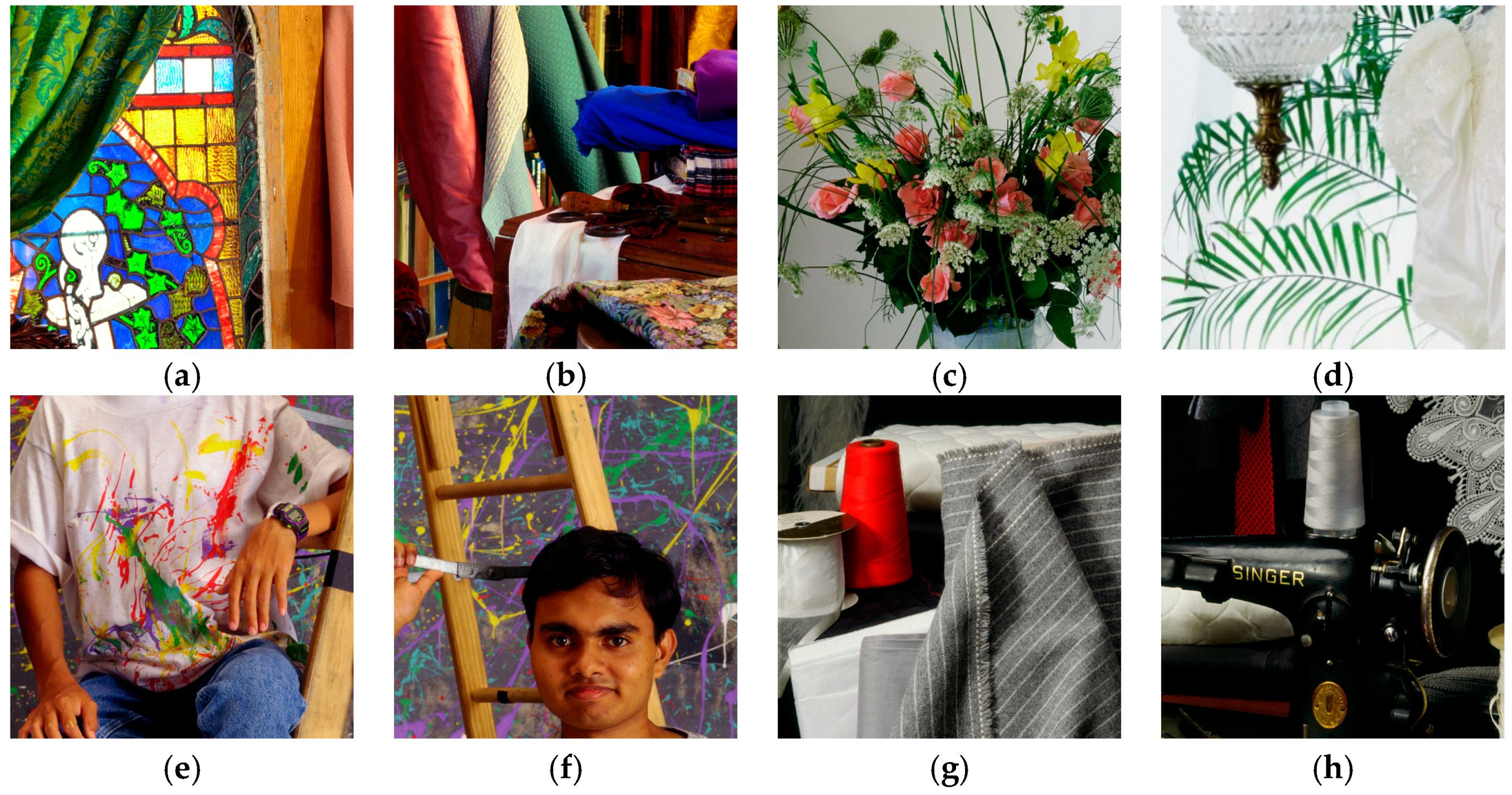
In this section, 18 images in the MCMaster dataset [29] are used to evaluate the effectiveness of the proposed algorithm. These images have a resolution of 500 × 500 as shown in Figure 6. The MCMaster dataset images are more in line with the characteristics of digital color images. The proposed algorithm is compared with DLMMSE [9], LDI-NAT [29], LDI-NLM [29], VDI [18], RI [19], and MLRI [21]. Especially, the guided filter is applied in the proposed algorithm, RI, and MLRI.

To simulate the proposed algorithm, we use MATLAB R2015b with Inter Core i7-5500U and 2.4 GHz CPU processors. Each calculation excludes the boundary of 10 pixels around the interpolated image in order to avoid the boundary effect.

Two indexes, peak signal-to-noise ratio (PSNR) and composite PSNR (CPSNR), are used to calculate the quality of the reconstructed demosaicking images, which are defined as:

$$\mathrm{PSNR}=10{\log }_{10}\left[\frac{{255}^2}{\frac{1}{MN}{\displaystyle \sum _{i=1}^M{\displaystyle \sum _{j=1}^N{\left[I_{\mathrm{in}}(i,j)-I_{\mathrm{out}}(i,j)\right]}^2}}}\right](\mathrm{dB}),$$

(17)

and

$$\mathrm{CPSNR}=10{\log }_{10}\left[\frac{{255}^2}{\frac{1}{3MN}{\displaystyle \sum _{k=1}^3{\displaystyle \sum _{i=1}^M{\displaystyle \sum _{j=1}^N{\left[I_{\mathrm{in}}(i,j,k)-I_{\mathrm{out}}(i,j,k)\right]}^2}}}}\right](\mathrm{dB}),$$

(18)

where $M$ and $N$ are the row and column sizes of image; $I_{\mathrm{in}}$ and $I_{\mathrm{out}}$ are the input image and the output image, respectively; $i$ and $j$ are the locations of pixels in the color plane, and $k$ represents the color plane.

Table 2. The PSNR (dB) of G components for the MCMaster images.

Image	DLMMSE [9]	LDI-NAT [29]	LDI-NLM [29]	VDI [18]	RI [19]	MLRI [21]	Proposed
Figure 6a	27.51	32.66	32.31	32.57	32.37	32.39	32.64
Figure 6b	31.91	39.00	39.09	38.95	39.44	39.24	39.47
Figure 6c	34.46	35.46	35.50	35.44	36.75	36.68	36.38
Figure 6d	36.80	40.40	38.99	41.31	42.14	41.16	43.15
Figure 6e	32.48	38.05	37.61	38.13	37.86	37.69	38.73
Figure 6f	33.09	43.36	41.87	42.49	42.16	41.85	43.12
Figure 6g	40.54	37.24	37.58	36.63	38.77	39.34	37.34
Figure 6h	40.43	40.15	40.32	39.60	41.37	41.73	40.36
Figure 6i	32.27	41.63	41.49	41.90	41.62	41.54	41.97
Figure 6j	31.15	42.66	42.24	42.47	42.07	41.98	42.95
Figure 6k	31.87	42.73	42.00	41.78	42.03	42.05	41.97
Figure 6l	31.55	41.52	41.52	41.65	42.24	42.04	42.38
Figure 6m	33.54	44.80	45.50	45.38	45.10	44.87	45.77
Figure 6n	30.89	42.80	42.62	42.96	43.05	42.78	43.71
Figure 6o	32.19	42.65	42.51	42.54	42.67	42.48	43.00
Figure 6p	26.70	35.60	35.10	35.20	35.16	35.28	35.35
Figure 6q	29.28	37.74	37.49	37.86	37.38	36.90	38.16
Figure 6r	30.43	37.66	37.74	36.36	37.68	37.89	36.89
Average	32.62	39.78	39.53	39.62	39.99	39.88	40.19

shows the PSNR of different algorithms to G components, since G components are the peak sensitivity of HVS. The highest PSNR of each image is marked in bold.

Table 3. The CPSNR (dB) of MCMaster images.

Image	DLMMSE [9]	LDI-NAT [29]	LDI-NLM [29]	VDI [18]	RI [19]	MLRI [21]	Proposed
Figure 6a	24.12	29.01	28.70	28.02	28.98	28.87	29.37
Figure 6b	28.39	35.01	34.86	34.16	35.00	35.09	35.17
Figure 6c	31.78	32.57	33.08	32.63	33.71	33.79	33.72
Figure 6d	34.13	35.95	36.47	36.00	37.88	37.48	38.56
Figure 6e	28.55	34.10	33.77	32.63	33.92	33.79	34.59
Figure 6f	29.24	37.86	37.12	35.64	38.32	38.29	38.62
Figure 6g	38.38	35.98	36.28	36.03	36.97	37.43	36.00
Figure 6h	36.64	37.46	37.82	37.41	36.98	36.83	38.20
Figure 6i	28.85	36.91	36.98	35.96	35.92	36.53	36.69
Figure 6j	27.76	38.73	38.36	37.26	38.15	38.55	38.92
Figure 6k	28.66	39.47	39.19	37.96	39.43	39.96	39.74
Figure 6l	27.35	38.89	38.59	37.10	39.64	39.67	39.58
Figure 6m	29.10	40.78	40.85	39.41	40.31	40.53	40.71
Figure 6n	27.25	38.68	38.48	37.32	38.95	38.74	39.16
Figure 6o	28.78	38.93	38.94	37.85	38.35	38.92	39.27
Figure 6p	24.23	33.50	32.98	31.41	35.15	35.16	35.30
Figure 6q	26.39	32.83	32.54	31.16	32.39	32.48	33.26
Figure 6r	27.83	34.98	35.21	34.24	36.48	36.23	35.95
Average	29.30	36.20	36.12	35.12	36.47	36.57	36.82

shows the CPSNR of different algorithms. The highest CPSNR of each image is marked in bold.

As shown in Table 2, the proposed algorithm performs better than the other six algorithms on 10 out of 18 images. The average PSNR of G components in the proposed algorithm is higher than MLRI and RI by 0.31 dB and 0.20 dB, respectively. Moreover, as for CPSNR in Table 3, the proposed algorithm performs better than the other six algorithms on 11 out of 18 images. The average CPSNR of the proposed algorithm is higher than that of MLRI and RI by 0.35 dB and 0.25 dB, respectively. In brief, among the three methods, RI [19], MLRI [21], and the proposed algorithm, those use the guided filter, the proposed algorithm is superior to MLRI and RI. This demonstrates that the proposed algorithm is effective for image demosaicking.

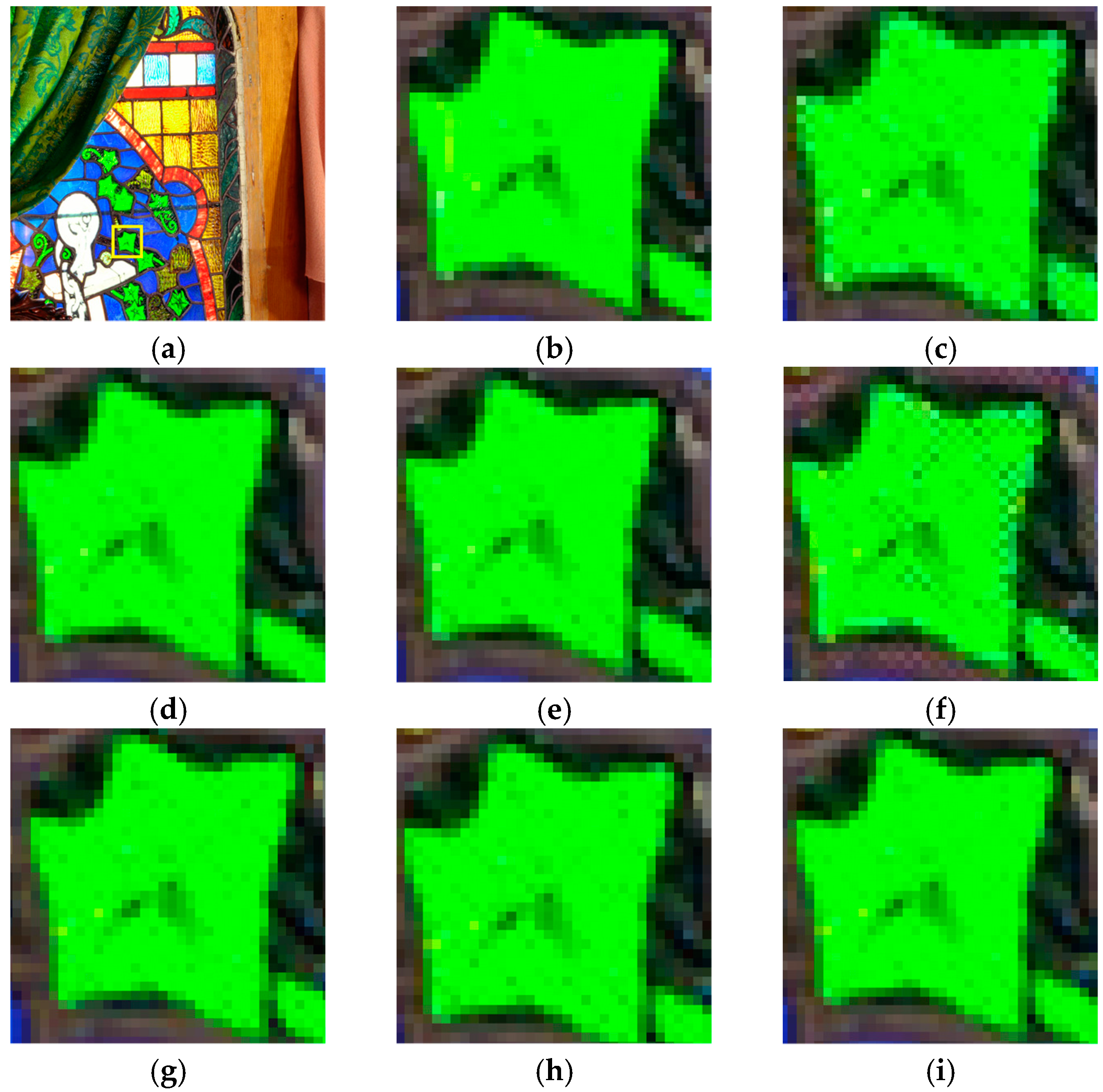
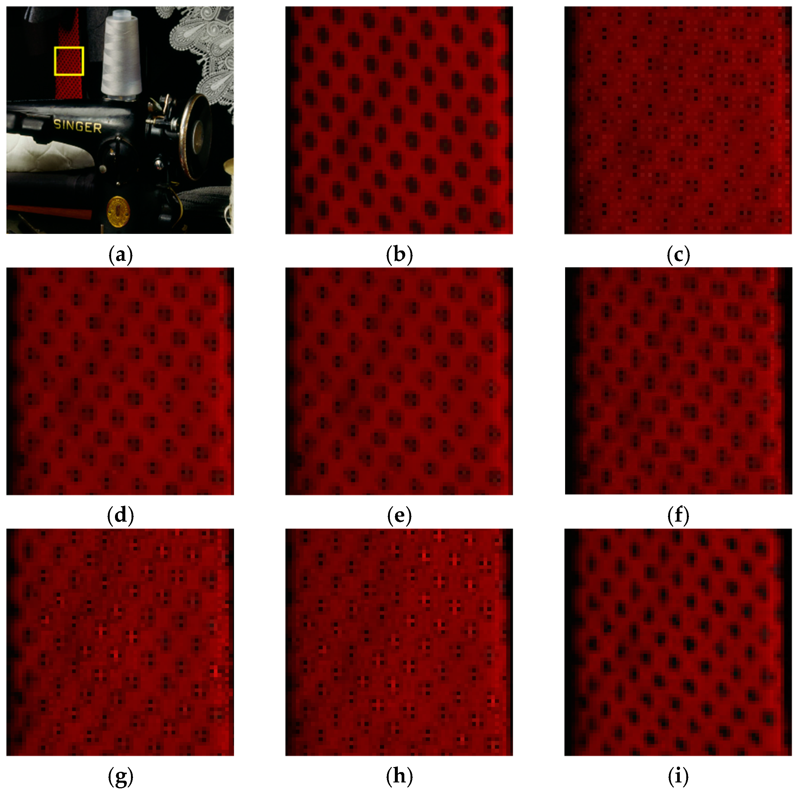
Objective measures are not reliable enough to judge the performance of the proposed method sometimes. Thus, we choose Figure 6a,h to show visual comparison of the interpolated images. Figure 7 shows the visual comparison of the yellow rectangular frame in Figure 6a. Figure 8 shows the visual comparison of the yellow rectangular frame in Figure 6h. We can find that the proposed algorithm produces precise image color information in details. In Figure 7, the Figure 7i has fewer artifacts than other subfigures. In Figure 8, the Figure 8i reconstructs the dots more exactly than other subfigures.

We use CPU processing time to compare computational complexity. The original source codes of [9,19,21,29] are used to record the CPU processing time under the same test conditions. The average computation time for each method is shown in

Table 4. Average computation time (s) on MCMaster images.

DLMMSE [9]	LDI-NAT [29]	LDI-NLM [29]	VDI [18]	RI [19]	MLRI [21]	Proposed
6.68	397.94	66.90	1.96	1.20	1.57	1.50

. For each image, the proposed algorithm takes 1.50 s while MLRI takes 1.57 s. The proposed algorithm reduces two directional-weight calculation processes. Therefore, it shows lower complexity. LDI-NAT and LDI-NLM take more than 60 s in the same condition because of the nonlocal mean method that is used to refine the interpolation. To sum up, the proposed algorithm provides a relatively low computational complexity.

5. Conclusions

In this paper, an effective directional residual interpolation algorithm for color image demosaicking is presented. With the use of directional weights by residual interpolation, more precise color components are interpolated. The proposed algorithm can be an alternative to color difference interpolation and MLRI, because it provides lower computational complexity by using horizontal and vertical weights. Besides, based on calculating the color difference estimations, we use a novel method to effectively reduce the influence of false edge information in irregular edges. It provides better color fidelity. Experimental results show that the proposed algorithm has outstanding performance on more complicated edge areas with lower computational complexity. In addition, it shows better subjective quality. For further work, we will continue to focus on the improved algorithm with better visual effect on more types of images. However, this improvement does not necessarily make the estimated values closest to the true values. Therefore, future research efforts will focus on finding an optimal algorithm to remove the difference caused by the directional color difference estimations absolutely.

References

- Gunturk, B.K.; Glotzbach, J.; Altunbasak, Y.; Schafer, R.W.; Mersereau, R.M. Demosaicking: Color filter array interpolation. IEEE Signal Process. Mag. 2005, 22, 44–54. [Google Scholar] [CrossRef]
- Bayer, B.E. Color Imaging Array. U.S. Patent 3,971,065, 20 July 1976. [Google Scholar]
- Adams, J.E. Interactions between color plane interpolation and other image processing functions in electronic photography. In Proceedings of the SPIE—Cameras and Systems for Electronic Photography and Scientific Imaging, San Jose, CA, USA, 8–9 February 1995; Volume 2416, pp. 144–151. [Google Scholar]
- Longère, P.; Zhang, X.; Delahunt, P.B.; Brainard, D.H. Perceptual assessment of demosaicing algorithm performance. Proc. IEEE 2002, 90, 123–132. [Google Scholar] [CrossRef]
- Yu, W. Colour demosaicking method using adaptive cubic convolution interpolation with sequential averaging. IEE Proc. Vis. Image Signal Process. 2006, 153, 666–676. [Google Scholar] [CrossRef]
- Malvar, H.S.; He, L.W.; Cutler, R. High-quality linear interpolation for demosaicing of Bayer-patterned color images. In Proceedings of the IEEE International Conference on Acoustics, Speech, and Signal Processing, Montreal, QC, Canada, 17–21 May 2004; Volume 3, pp. 485–488. [Google Scholar]
- Yu, T.; Hu, W.; Xue, W.; Zhang, W. Colour image demosaicking via joint intra and inter channel information. Electron. Lett. 2016, 52, 605–607. [Google Scholar] [CrossRef]
- Zhang, C.; Li, Y.; Wang, J.; Hao, P. Universal demosaicking of color filter arrays. IEEE Trans. Image Process. 2016, 25, 5173–5186. [Google Scholar] [CrossRef] [PubMed]
- Zhang, L.; Wu, X. Color demosaicking via directional linear minimum mean square-error estimation. IEEE Trans. Image Process. 2005, 14, 2167–2178. [Google Scholar] [CrossRef] [PubMed]
- Wachira, K.; Mwangi, E. A multi-variate weighted interpolation technique with local polling for Bayer CFA demosaicking. In Proceedings of the 1st International Conference on Information and Communication Technology Research, Abu Dhabi, UAE, 17–19 May 2015; pp. 76–79. [Google Scholar]
- Shi, J.; Wang, C.; Zhang, S. Region-adaptive demosaicking with weighted values of multidirectional information. J. Commun. 2014, 9, 930–936. [Google Scholar] [CrossRef]
- Chen, W.J.; Chang, P.Y. Effective demosaicking algorithm based on edge property for color filter arrays. Digit. Signal Process. 2012, 22, 163–169. [Google Scholar] [CrossRef]
- Pekkucuksen, I.; Altunbasak, Y. Edge strength filter based color filter array interpolation. IEEE Trans. Image Process. 2012, 21, 393–397. [Google Scholar] [CrossRef] [PubMed]
- Tsai, C.Y.; Song, K.T. A new edge-adaptive demosaicing algorithm for color filter arrays. Image Vis. Comput. 2007, 25, 1495–1508. [Google Scholar] [CrossRef]
- Adams, J.E.; Hamilton, J.F. Adaptive Color Plan Interpolation in Single Sensor Color Electronic Camera. U.S. Patent 5,629,734, 13 May 1997. [Google Scholar]
- Pekkucuksen, I.; Altunbasak, Y. Gradient based threshold free color filter array interpolation. In Proceedings of the 17th IEEE International Conference on Image Processing, Hong Kong, China, 26–29 September 2010; pp. 137–140. [Google Scholar]
- Pekkucuksen, I.; Altunbasak, Y. Multiscale gradients-based color filter array interpolation. IEEE Trans. Image Process. 2013, 22, 157–165. [Google Scholar] [CrossRef] [PubMed]
- Chen, X.; Jeon, G.; Jeong, J. Voting-based directional interpolation method and its application to still color image demosaicking. IEEE Trans. Circuits Syst. Video Technol. 2014, 24, 255–262. [Google Scholar] [CrossRef]
- Kiku, D.; Monno, Y.; Tanaka, M.; Okutomi, M. Residual interpolation for color image demosaicking. In Proceedings of the 20th IEEE International Conference on Image Processing, Melbourne, Australia, 15–18 September 2013; pp. 2304–2308. [Google Scholar]
- Kiku, D.; Monno, Y.; Tanaka, M.; Okutomi, M. Beyond color difference: Residual interpolation for color image demosaicking. IEEE Trans. Image Process. 2016, 25, 1288–1300. [Google Scholar] [CrossRef] [PubMed]
- Kiku, D.; Monno, Y.; Tanaka, M.; Okutomi, M. Minimized-Laplacian residual interpolation for color image demosaicking. In Proceedings of the SPIE—IS and T Electronic Imaging—Digital Photography X, San Francisco, CA, USA, 3–5 February 2014; Volume 9023, pp. 1–8. [Google Scholar]
- Ye, W.; Ma, K.K. Color image demosaicing using iterative residual interpolation. IEEE Trans. Image Process. 2015, 24, 5879–5891. [Google Scholar] [CrossRef] [PubMed]
- Wang, L.; Jeon, G. Bayer pattern CFA demosaicking based on multi-directional weighted interpolation and guided filter. IEEE Signal Process. Lett. 2015, 22, 2083–2087. [Google Scholar] [CrossRef]
- Kim, Y.; Jeong, J. Four-direction residual interpolation for demosaicking. IEEE Trans. Circuits Syst. Video Technol. 2016, 26, 881–890. [Google Scholar] [CrossRef]
- Monno, Y.; Kiku, D.; Tanaka, M.; Okutomi, M. Adaptive residual interpolation for color and multispectral image demosaicking. Sensors 2017, 17, 2787. [Google Scholar] [CrossRef] [PubMed]
- He, K.; Sun, J.; Tang, X. Guided image filtering. IEEE Trans. Pattern Anal. Mach. Intell. 2013, 35, 1397–1409. [Google Scholar] [CrossRef] [PubMed]
- Monno, Y.; Kiku, D.; Kikuchi, S.; Tanaka, M.; Okutomi, M. Multispectral demosaicking with novel guide image generation and residual interpolation. In Proceedings of the IEEE International Conference on Image Processing, Paris, France, 27–30 October 2014; pp. 645–649. [Google Scholar]
- Oh, P.; Lee, S.; Kang, M.G. Colorization-based RGB-white color interpolation using color filter array with randomly sampled pattern. Sensors 2017, 17, 1523. [Google Scholar] [CrossRef] [PubMed]
- Zhang, L.; Wu, X.; Buades, A.; Li, X. Color demosaicking by local directional interpolation and nonlocal adaptive thresholding. J. Electron. Imaging 2011, 20, 1–16. [Google Scholar]
Figure 1.
Bayer pattern CFA.
Figure 2.
The interpolation of the R pixel values by using MLRI.
Figure 3.
The outline of the proposed algorithm.
Figure 4.
The horizontal R pixel value interpolation: (a) Adams and Hamilton’s interpolation equation [15]; (b) MLRI [21].
Figure 5.
The calculation process of the directional weights.
Figure 6.
The MCMaster dataset images.
Figure 7.
The processing results of image Figure 6a: (a) the original image marked with the yellow rectangular frame; (b) the enlarged area of the yellow rectangular frame; (c) DLMMSE [9]; (d) LDI-NAT [29]; (e) LDI-NLM [29]; (f) VDI [18]; (g) RI [19]; (h) MLRI [21]; (i) the proposed algorithm.
Figure 8.
The processing results of image Figure 6h: (a) the original image marked with the yellow rectangular frame; (b) the polka dots of the tie in the yellow rectangular frame; (c) DLMMSE [9]; (d) LDI-NAT [29]; (e) LDI-NLM [29]; (f) VDI [18]; (g) RI [19]; (h) MLRI [21]; (i) the proposed algorithm.