Noise Attenuation Based on Wave Vector Characteristics

Abstract

Polarization filtering has been widely used to enhance signal-to-noise ratios for multicomponent seismic data. Polarization filters routinely depend on the ellipticity and directionality of spatial particle motions. However, factors such as noise and formation heterogeneity often make the polarization characteristics of body waves hard to distinguish. Here, we introduce a technique in the time domain for the separation of valid body waves and noise based on wave vector characteristics. First, we characterise the ground-roll polarization by the median wave vectors derived in large-scale moving time windows. For the suppression of ground roll, we fit the particle trajectory of ground roll by the least square method using all components simultaneously. Second, we apply three-stage smoothing to the ground-roll-removed multicomponent records. In each stage, we use mean or median vectors derived in small-scale moving-time or moving-trace windows to attenuate random noise and other non-ground-roll related coherent noise. The filter in the proposed method is not devised according to ellipticity and directionality. Instead, we use the wave vector decomposition to distinguish between noise and valid signals. Synthetic data and field data examples confirm that the proposed method can effectively suppress noise without damaging the high and low frequencies of a valid signal.

1. Introduction

Multicomponent geophones can fully record the spatial particle motions of elastic wavefields. Using the full vector amplitude information of the elastic wavefield is beneficial for reservoir prediction and fluid detection. Therefore, it is important to maintain the wave vector information of the elastic wavefield during multicomponent data processing [1]. To avoid damaging the vector fidelity of valid seismic signals, multicomponent seismic acquisition usually adopts a single-point non-combination receiving mode [2], which also results in a lower signal-to-noise ratio (S/N) for the multicomponent seismic data.

Many existing denoising methods can be directly applied to multicomponent seismic data to improve the S/N; however, most are aimed at single component data. The most appropriate denoising method to apply depends on the valid signal energy and S/N. In most cases, the vertical Z-component has a higher S/N, while the horizontal component has a poorer S/N. Therefore, conventional denoising methods are not adequate for maintaining vector amplitude information because of the variability of filtering parameters and the variability of signal and noise on each component [3]. Keeping vector amplitude information during denoising remains a challenge to multicomponent seismic data processing.

Polarization filtering is a method that separates valid signals from noise by using vector amplitude measured on three-component (3C) records [4,5]. Polarization filtering has been studied for decades [4,6,7,8,9,10,11], with most studies based on ellipticity or direction filters [3,4]. For such filtering methods, it is often assumed that ground roll tends to appear as elliptical polarization in the vertical plane, while body waves are linearly polarised in three-dimensional space and random noise is unpolarised [12,13,14]. Valid Signals are separated from the noise background based on predefined polarization attributes such as ellipticity or polarization direction.

Polarization attributes are usually derived in the time domain or in the frequency (or the time-frequency) domain. In the time domain, most techniques are based on an eigenanalysis of the data matrix constructed within a given moving time window over two-component (2C) or 3C data [12]. One can determine the polarization type according to the semi-major and semi-minor axes of the polarization trajectory given by the eigenvalues of the data covariance matrix [3] or by the eigen images of singular-value decomposition (SVD) on the data matrix [15,16]. The success of these techniques depends on the selection of the moving window, which is affected by the dominant period, S/N, and polarization type. The problem faced by polarization filtering in the time domain is that valid signals and noise with a similar period arriving in the same time window are hard to decompose [13].

To deal with a wavefield decomposition with different frequency contents, polarization filtering based on frequency attributes has been developed. Samson described a method of estimating the polarization as a function of frequency [17]. Park et al. devised a multitaper algorithm to determine the polarization of particle motion as a function of frequency and applied it to filter field 3C data [18]. Du et al. developed the multitaper spectral method of Park et al. to derive a data-adaptive polarization filter based on the estimation of the spectral density matrix [10,18]. However, some noise, such as ground roll, always shares a similar frequency band with shear waves. To overcome this problem, polarization-filtering methods in the time-frequency domain are employed rather than those in a real time-series to separate noise and body waves [5,11,19,20,21,22,23,24]. However, body waves are still hard to distinguish only using instantaneous polarization attributes when significant random noise and extra non-ground-roll related coherent noise occur on all three components [25]. In addition, ground roll easily loses its original elliptical polarization during propagation owing to the anisotropy and inhomogeneity of the near surface. Therefore, extra constraints need to be added into polarization filtering to improve discrimination among different polarization modes.

In this study, we develop a noise attenuation method based on mean and median filtering of wave vectors, which, in turn, may be thought of as evolved from the pioneering works of Schimmel and Gallart, Hou et al., and Liu [5,26,27]. The proposed method is implemented in moving windows at different scales in the time domain. At each time sample, we consider the wave vector to be composed by the valid-signal vector, the ground-roll vector, the random-noise vector and other noise vectors (e.g., the vector of non-ground-roll related coherent noise). We devise two different smoothing approaches to separate the ground-roll polarization and the body-wave polarization from the random noise background. Our filter does not depend on ellipticity or directionality and does not require setting up any kind of data covariance matrices or complex traces. Tests of our noise attenuation method show it to be effective with numerical and field data examples.

2. Principles

2.1. Wave Vector Estimation

In a three-dimensional (3D) 3C seismic survey, translational motions are simultaneously recorded by one vertical (Z-) component and two horizontal (X- and Y-) components of the geophone [1]. The 3C amplitudes u_Z, u_X, and u_Y at the sample time t form a signal vector:

$$\mathbf{U}\left(t\right)=u_Z\left(t\right){\mathbf{e}}_Z+u_X\left(t\right){\mathbf{e}}_X+u_Y\left(t\right){\mathbf{e}}_Y$$

(1)

where e_Z, e_X, and e_Y are base (unit) vectors in the Z-, X-, and Y-directions, respectively. To the isotropic exploration target, when the X-component is rotated to the receiver-source (radial) direction, valid seismic waves are mainly recorded by the Z- and X-components. Thus, the vector U can be written as:

$$\mathbf{U}\left(t\right)=u_Z\left(t\right){\mathbf{e}}_Z+u_X\left(t\right){\mathbf{e}}_X$$

(2)

At the given time t, U(t) is not a pure vector of a valid wave owing to the existence of different noises as ground roll, random noise, and other kinds of noise. Rather, it is a composite vector approximately expressed as:

$$\mathbf{U}\left(t\right)=\mathbf{B}\left(t\right)+\mathbf{G}\left(t\right)+\mathbf{N}\left(t\right)$$

(3)

where B(t), G(t) and N(t) are the wave vectors of a valid signal, ground roll, and random noise together with other non-ground-roll related coherent noise, respectively, and

$$\{\begin{array}{l}\mathbf{B}\left(t\right)=B\left(t\right){\mathbf{e}}_B\\ \mathbf{G}\left(t\right)=G\left(t\right){\mathbf{e}}_G\\ \mathbf{N}\left(t\right)=N\left(t\right){\mathbf{e}}_N\end{array}$$

(4)

where e_B, e_G, and e_N are the unit wave vectors; and B(t), G(t), and N(t) denote the wave vector moduli. Here, the non-ground-roll related coherent noise refers to the linear noise without dispersion.

Through analysis of a 3C record using a moving window, we can derive a mean (or median) vector that characterises the polarization in the moving window [5]. The moving window size can be tailored for different applications and statistics. For instance, using a large moving window can produce the near-zero random-noise vector moduli and relatively accurate instantaneous ground-roll vectors. Using a small moving window can produce the opposite effect. Based on the wave vector characteristics of different moving windows, we consider using mean (or median) filtering to reduce the noise in 3C records.

2.2. Ground Roll Attenuation

Ground roll propagates close to the surface in low-velocity strata with high-amplitude and low frequency elliptical polarization [16]. To separate the wave vectors of ground roll, we add a large-scale moving time window to the 3C record and calculate the median wave vector from a mean vector set in order to characterize the ground roll polarization [5]. Within time window T₁, each mean wave vector K_j is calculated by:

$${\mathbf{K}}_j=\begin{array}{cc}\frac{\mathbf{U}\left(t-T_1/2+j\Delta t\right)+\mathbf{U}\left(t+T_1/2-j\Delta t\right)}{2}& j=0,\dots ,\frac{T_1}{2\Delta t}\end{array}$$

(5)

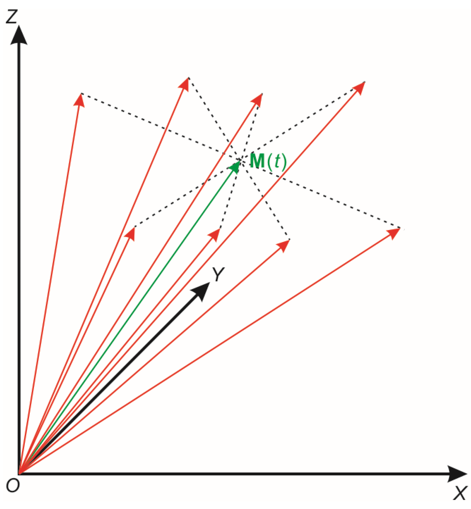
These mean vectors form a 1 + T₁/(2Δt) dimensional vector set, in which each element is close to the true wave vector at the time t. Then, we calculate the total distance of one mean vector to all the other mean vectors by:

$$\begin{array}{cc}D\left({\mathbf{K}}_j\right)={\displaystyle \sum _{i=0}^{\frac{T_1}{2\Delta t}}{\Vert {\mathbf{K}}_j-{\mathbf{K}}_i\Vert }_2}& \begin{array}{cc}j=0,\dots ,\frac{T_1}{2\Delta t},& i\ne j\end{array}\end{array}$$

(6)

The median vector is derived by a median filter [26,27]:

$$\begin{array}{cc}\mathbf{M}\left(t\right)=\mathrm{argmin}\left(D\left({\mathbf{K}}_j\right)\right)& \begin{array}{cc}j=0,\dots ,\frac{T_1}{2\Delta t},& i\ne j\end{array}\end{array}$$

(7)

As shown in Figure 1, M(t) is located at the centre of the mean vector set and has a minimum total distance to all other mean vectors.

The median filter is a low-pass filter that can remove impulse noise by smoothing [28]. Therefore, median filters may also suppress sharp amplitudes in valid signals. To make up for this, we recover the vector moduli of the valid signal using a least squares method given by:

$$Q\left(t\right)={\displaystyle \sum _{\tau =t-T_1/2}^{t+T_1/2}{\left(\mathbf{U}\left(\tau \right)-{\gamma }_1\left(t\right)\mathbf{M}\left(\tau \right)\right)}^2}$$

(8)

where γ₁(t) is the scaling factor used to modify the median vector modulus. To minimize the objective function Q(t), we set:

$$\frac{\partial Q\left(t\right)}{\partial {\gamma }_1\left(t\right)}=0$$

(9)

Then, the scaling factor is derived as:

$${\gamma }_1\left(t\right)=\frac{{\displaystyle \sum _{\tau =t-T_1/2}^{t+T_1/2}\mathbf{U}\left(\tau \right)\cdot \mathbf{M}\left(\tau \right)}}{{\displaystyle \sum _{\tau =t-T_1/2}^{t+T_1/2}{\left(\mathbf{M}\left(\tau \right)\right)}^2}}$$

(10)

Therefore, the ground roll vector with a true modulus is:

$$\mathbf{G}\left(t\right)={\gamma }_1\left(t\right)\mathbf{M}\left(t\right)$$

(11)

Directly using the subtraction method according to Equation (2), we get a ground-roll-free wave vector time-series C(t) of

$$\mathbf{C}\left(t\right)=\mathbf{U}\left(t\right)-\mathbf{G}\left(t\right)=\mathbf{B}\left(t\right)+\mathbf{N}\left(t\right)$$

(12)

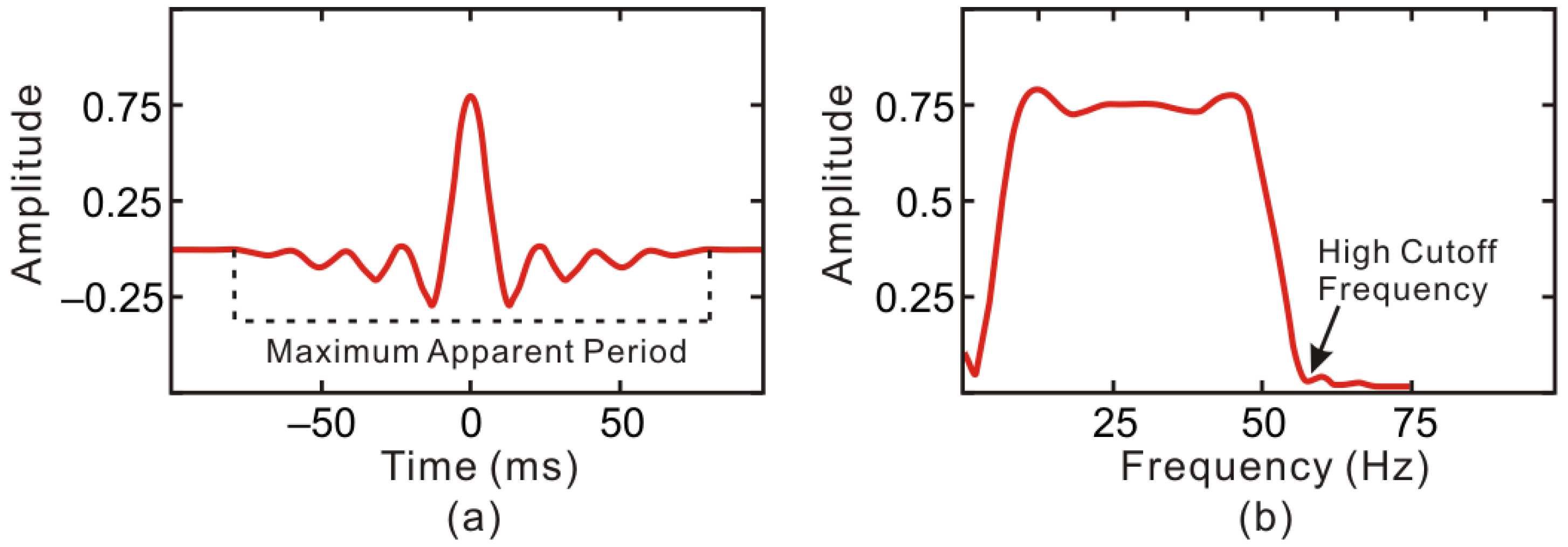
The proper moving time window size is crucial to the recovery of ground roll vector characteristics. During the calculation of the median vector for ground roll, both valid signals and random noise are dealt with as noise. The vector moduli of valid signals can be suppressed through median filtering only when the moving time window size is longer than the period of the valid signal (Figure 2a). Nevertheless, a too-large moving time window leads to poor suppression of the high-frequency part of ground roll. Therefore, we set the moving time window size to be close to the maximum apparent period of the valid signal.

2.3. Attenuation of Random Noise and Other Non-Ground-Roll Related Coherent Noise

Unlike ground roll, to suppress random noise and other non-ground-roll related coherent noise, we use smaller moving windows to maintain valid signal amplitudes. As shown in Figure 2b, the moving time window can be set to:

$$T_2=\frac{1}{2f_{\max }}$$

(13)

where f_max is the high cutoff frequency of the valid signal wavelet. Within the moving time window, we adopted a three-stage smoothing approach to extract pure valid body wave vectors. In the first stage, we use mean filtering to get the mean vector M₁(t):

$${\mathbf{M}}_{\mathbf{1}}\left(t\right)=\frac{1}{T_2+1}{\displaystyle \sum _{\tau =t-T_2/2}^{t+T_2/2}\mathbf{C}\left(t\right)}$$

(14)

Mean filtering superposes all the wave vectors within the moving time window and takes the mean vector for the centre. The superposition of wave vectors in the moving time window can highlight body-wave vectors and suppress noise vectors [29].

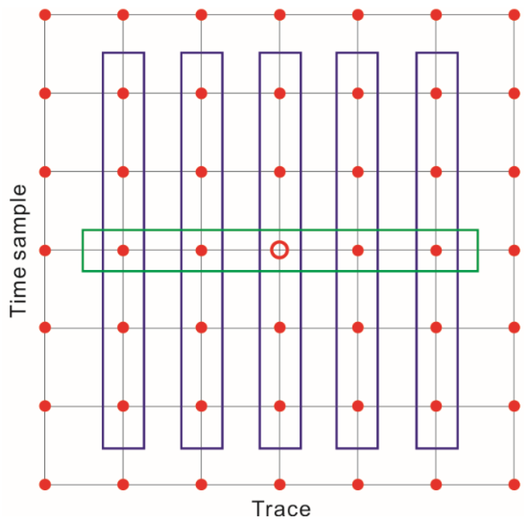
As shown in Figure 3, in the second stage, we perform median filtering over time (blue rectangle in Figure 3) at each trace for all wave vectors to suppress random noise vectors:

$$\begin{array}{cc}{\mathbf{M}}_{\mathbf{2}}\left(t\right)=\mathrm{argmin}\left({\displaystyle \sum _{i=t-T_2/\left(2\Delta t\right)}^{t+T_2/\left(2\Delta t\right)}{\Vert {{\mathbf{M}}_{\mathbf{1}}}_j-{{\mathbf{M}}_{\mathbf{1}}}_i\Vert }_2}\right)& \begin{array}{cc}j=t-\frac{T_2}{2\Delta t},\cdots ,t+\frac{T_2}{2\Delta t},& i\ne j\end{array}\end{array}$$

(15)

Then, in the third stage, we perform median filtering over trace (green rectangle in Figure 3) for the same sample to suppress non-ground-roll related coherent noise:

$$\begin{array}{ccc}{\mathbf{M}}_{\mathbf{3}}\left(l\right)=\mathrm{argmin}\left({\displaystyle \sum _{i=l-L/\left(2\Delta l\right)}^{l+L/\left(2\Delta l\right)}\Vert {{\mathbf{M}}_{\mathbf{2}}}_j-{{\mathbf{M}}_{\mathbf{2}}}_i\Vert }\right)& j=l-\frac{L}{2\Delta l},\cdots ,l+\frac{L}{2\Delta l},& i\ne j\end{array}$$

(16)

where l denotes the output trace of the median filtering and L is the size of the moving trace window. The median filtering over trace should be performed within the same seismic receiving line because only adjacent seismic traces in the same receiving line have similar wave vector characteristics. Then, we derive the pure valid signal vector by scaling the median vector M₃ as:

$$\mathbf{B}\left(t\right)={\gamma }_2\left(t\right){\mathbf{M}}_{\mathbf{3}}\left(t\right)$$

(17)

and

$${\gamma }_2\left(t\right)=\frac{{\displaystyle \sum _{\tau =t-T_2/2}^{t+T_2/2}\mathbf{C}\left(\tau \right)\cdot {\mathbf{M}}_{\mathbf{3}}\left(\tau \right)}}{{\displaystyle \sum _{\tau =t-T_2/2}^{t+T_2/2}{\left({\mathbf{M}}_{\mathbf{3}}\left(\tau \right)\right)}^2}}$$

(18)

3. Numerical Data Test

3.1. Numerical One-dimensioal Two-component Data

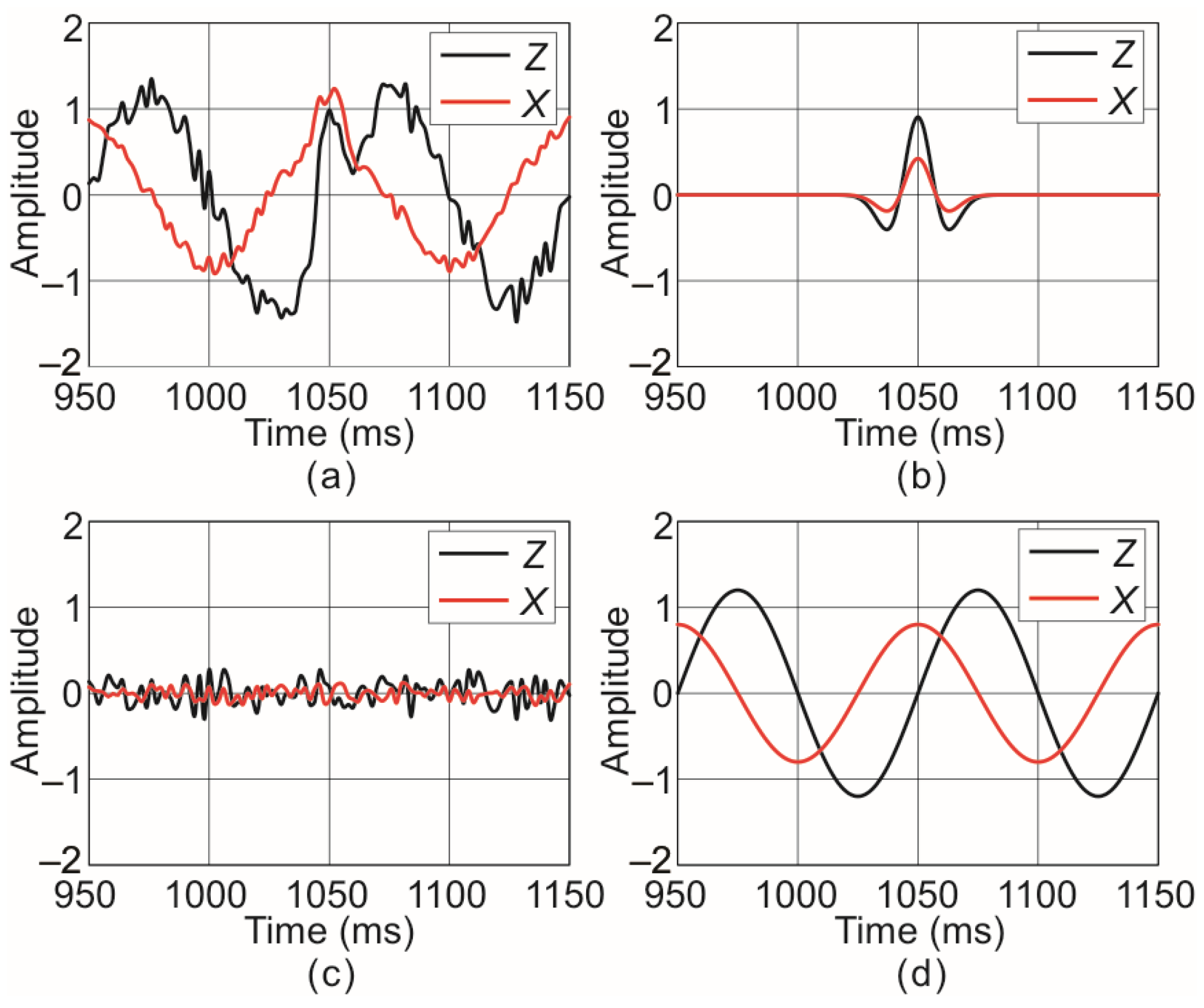
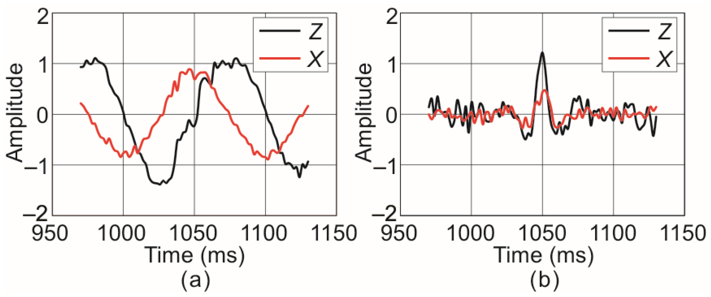
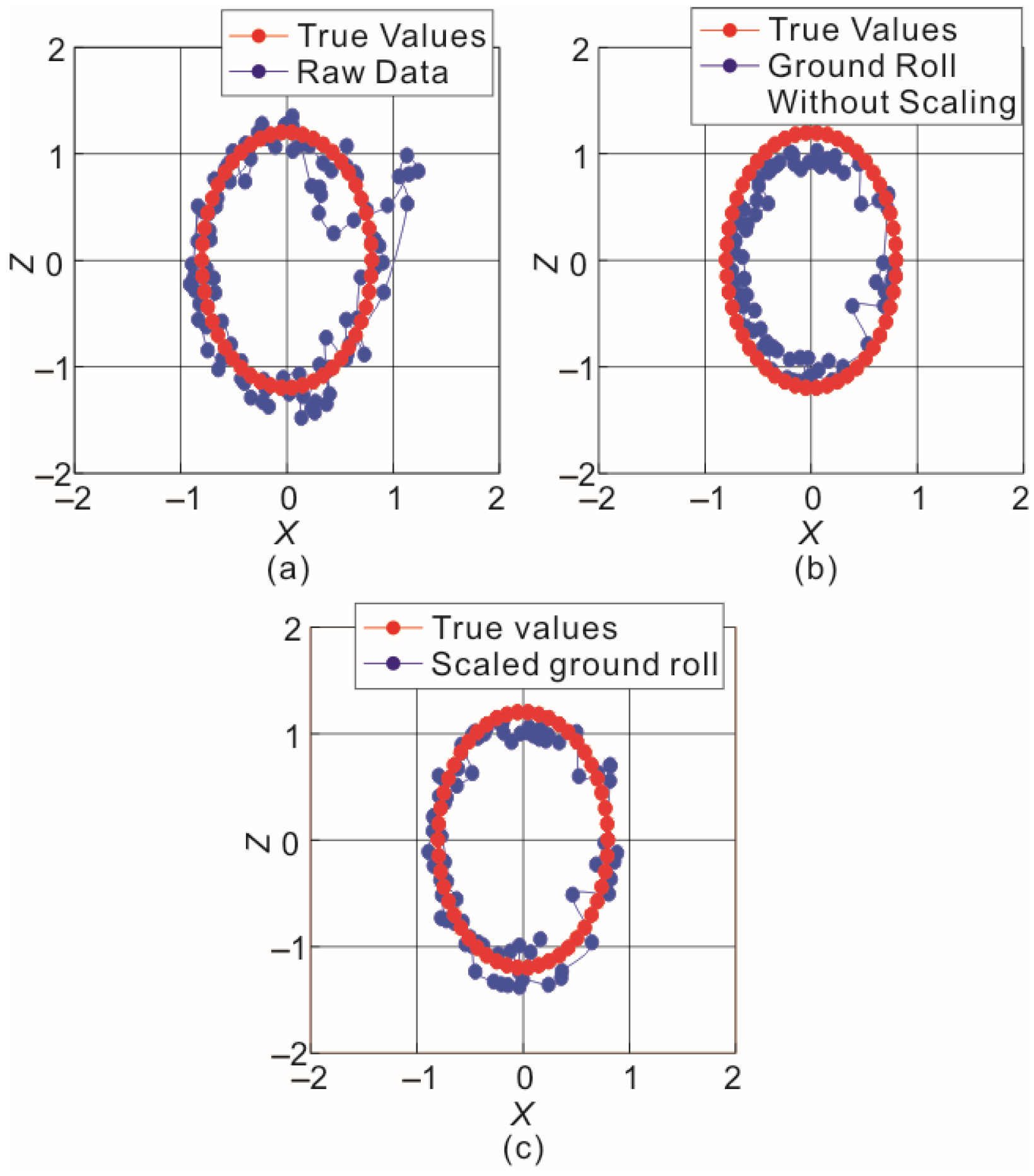
As shown in Figure 4, the synthetic one-dimensional two-component (1D2C) records (Figure 4a) for the test are generated with the valid seismic signal at a 30 Hz dominant frequency (Figure 4b) added by 50% (noise to signal energy ratio) random noise (Figure 4c) and strong ground roll (Figure 4d). It is clear that the apparent periods of the seismic signal and the ground roll are about 40 and 100 ms, respectively. As shown in Figure 5, we are able to well separate the ground roll (Figure 5a) and valid signal with random noise (Figure 5b) using a 40-ms moving time window. As shown in Figure 5, the data at the start and end 20 ms cannot be filtered because they are located at the start and end borders of the moving time window. The polarization hodograms in Figure 6 show that median filtering effectively improves the ellipticity of the ground roll because the body wave and noise vectors are reduced. However, with median filtering, the separated ground roll—without adopting any scaling factor—presents a smaller elliptical polarization trajectory (Figure 6b). The time-variant scaling factors can improve the matching of the polarization trajectories between the separated ground roll and the true one (Figure 6c).

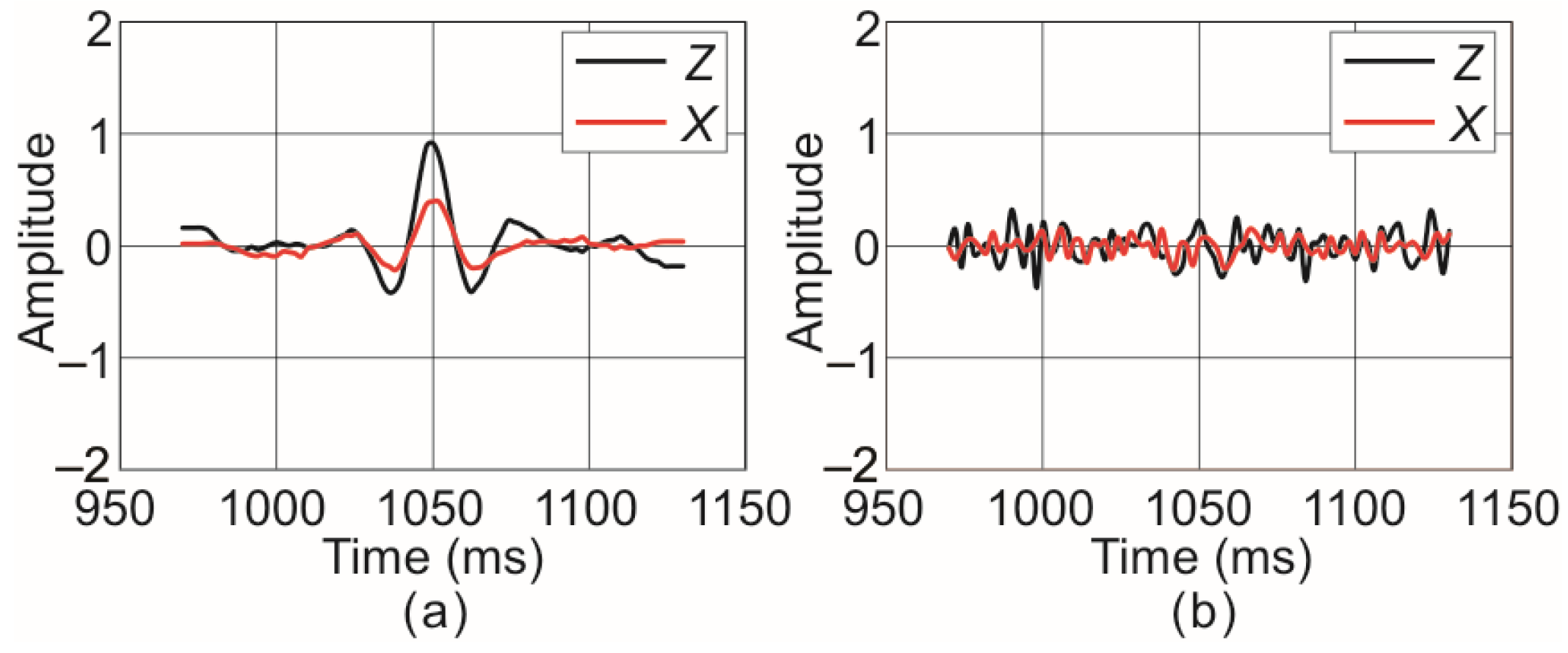
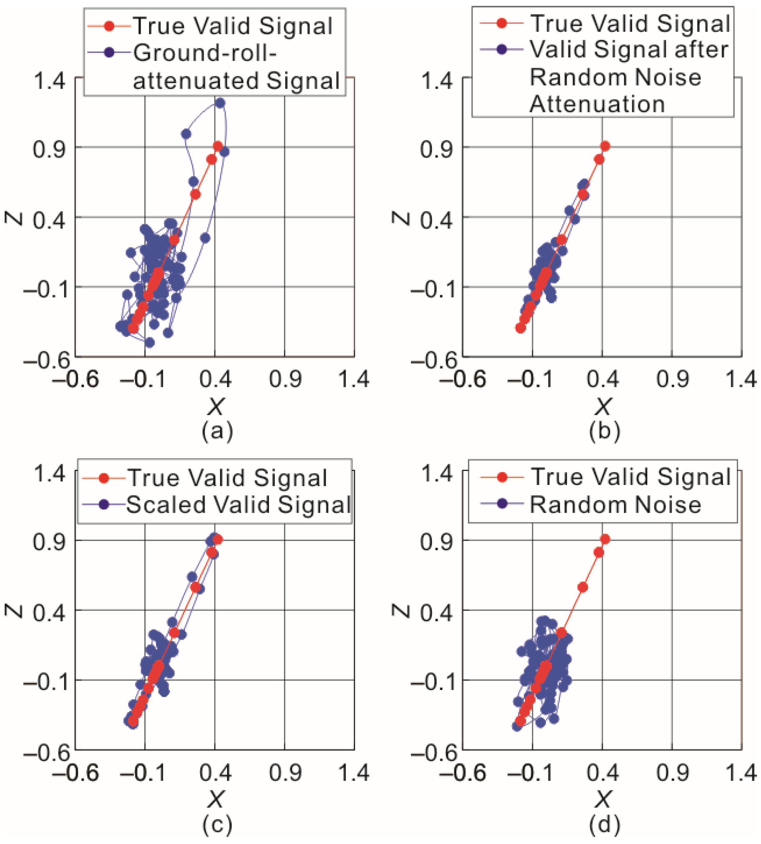
Then, we perform median filtering to the ground-roll-attenuated data using a 5-ms moving window to separate the valid signal (Figure 7a) and the random noise (Figure 7b). Figure 8 shows that our noise attenuation method can well distinguish between the body-wave and random-noise polarizations and recover the linear polarization of the body wave. Comparing Figure 8b with Figure 8c, it is clear that adopting scaling factors can make our noise attenuation method more amplitude preserving.

3.2. Two-dimensional Two-Component Synthetic Data

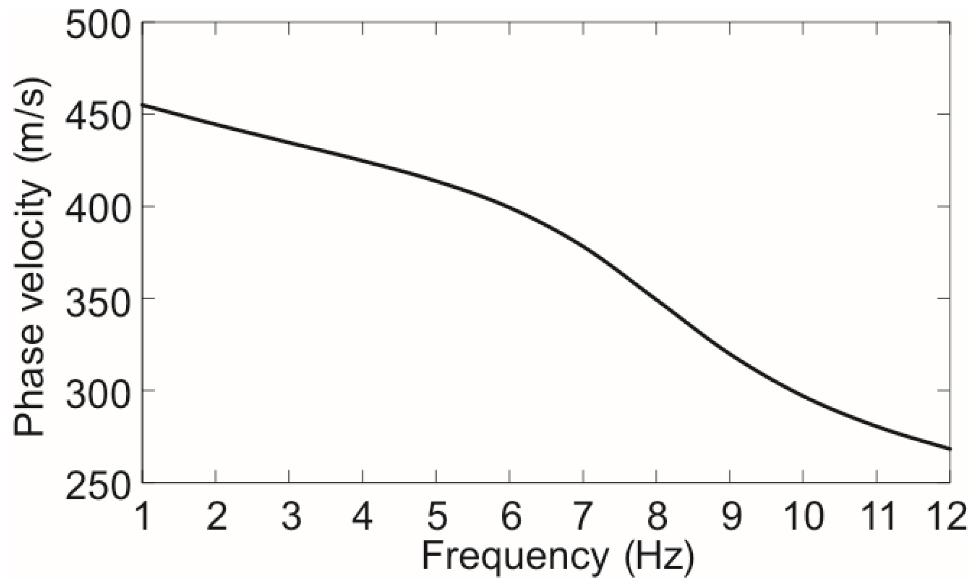
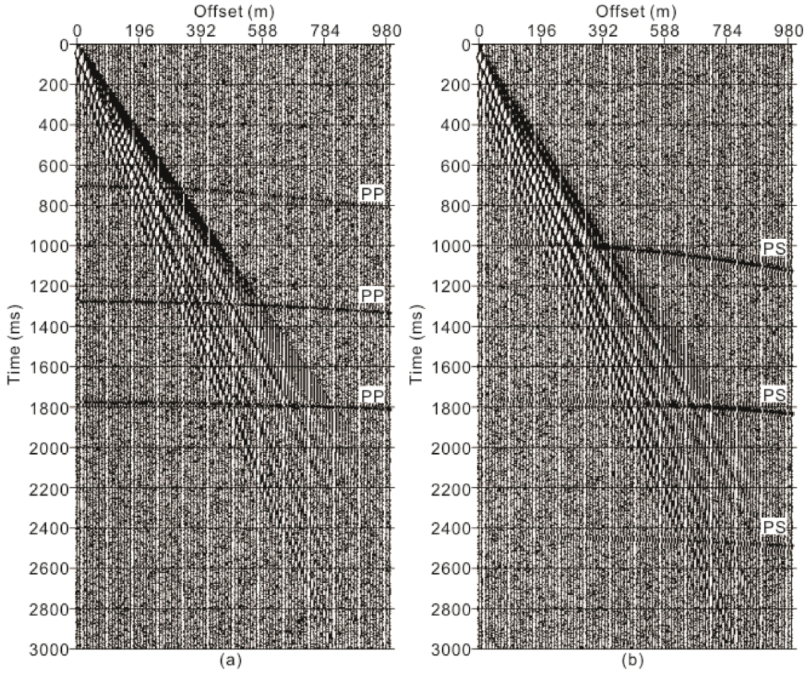
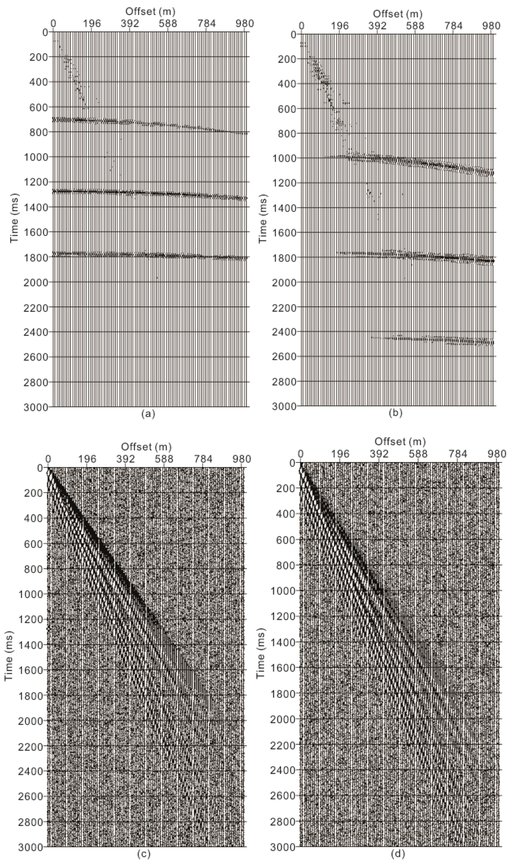
We apply our method to the synthetic shot records from the theoretical model shown in

Table 1. Theoretical model parameters.

Density (g/cm3)	Thickness (m)	P-Wave Velocity (m/s)	S-Wave Velocity (m/s)
1.47	5	500	200
1.53	5	600	300
1.74	30	1000	500
2.19	760	2500	1443
2.26	800	2800	1617
2.33	800	3200	1848
2.4	600	3600	2078

. The near-surface ground roll is numerically generated using the methods introduced by Knopoff and Schwab and PP- and PS-reflections from the deep interfaces are obtained by ray tracing [30,31,32]. The simulated ground roll is dispersive with a frequency band of 1–12 Hz (Figure 9). The frequency band of the added non-ground-roll related coherent noise is 10–20 Hz. The dominant frequencies of PP- and PS valid waves are 30 Hz and 15 Hz, respectively. Compared with the valid waves in the synthetic shot records (Figure 10a,b), the added ground roll is of 350% level (Figure 10c,d), the added non-ground-roll related coherent noise is of 50% level (Figure 10e,f), and the added random noise is of 400% level. The sample rate of the synthetic shot records is 1 ms and the maximum apparent period of the valid wave is 60 ms.

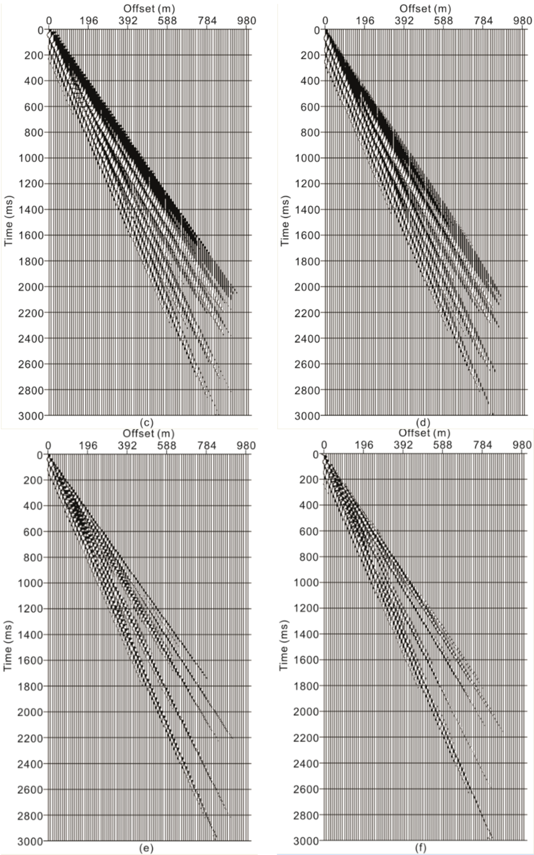
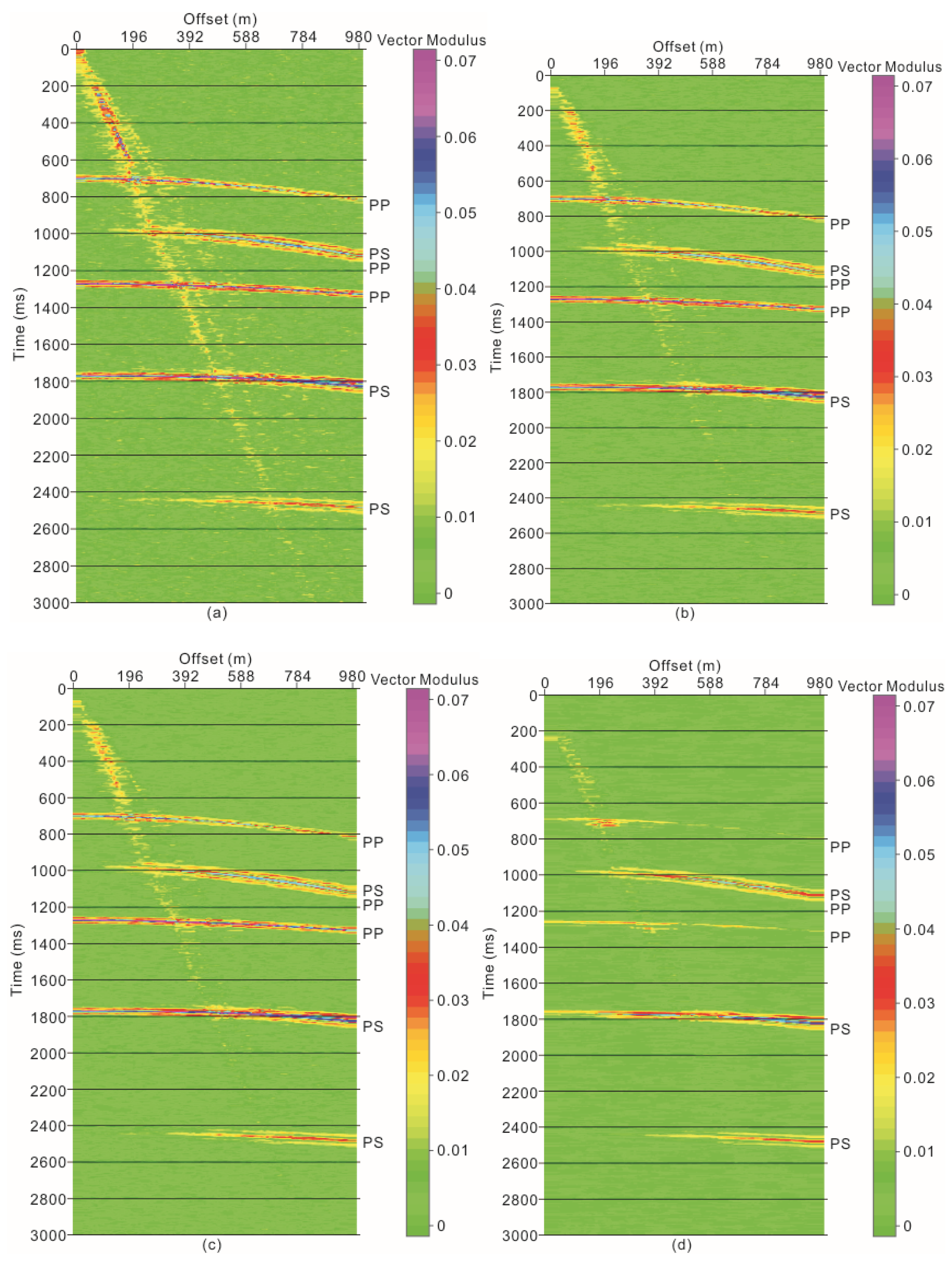
First, we determine the moving window size for the attenuation of ground roll according to the map of wave vector modulus (Figure 11). As shown in Figure 11a, a 50-ms moving window corresponding to the apparent period of the PP-wavelet can well suppress PP-wave vectors but can hardly differentiate between the PS-waves and ground-roll vectors. A 60-ms moving window (Figure 11b) is a little smaller than the apparent period of the PS-wavelet, so parts of the PS-vectors were left. The 70-ms moving window (Figure 11c) is exactly equal to the apparent period of the PS-wavelet, and perfectly highlighted the wave vectors of the ground roll and suppressed both the PP- and PS-vectors. As shown in Figure 11d, too-large time windows (e.g., 80 ms) caused high-frequency ground roll to be less recognizable, although valid wave vectors are well suppressed. After testing, we choose the 70-ms moving window for the separation of the ground roll.

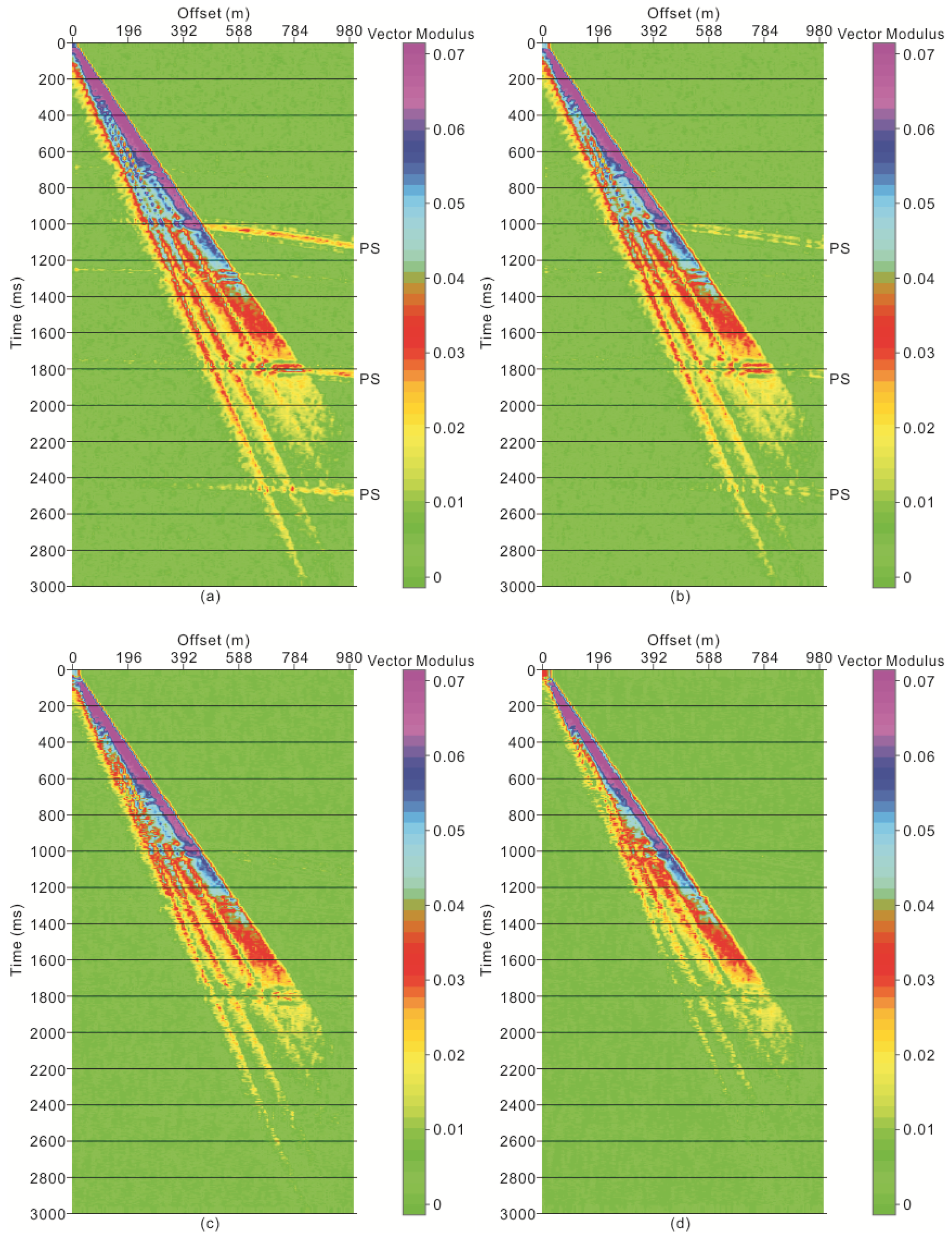
Second, we test different moving time and moving trace windows based on the ground-roll-attenuated data. As the cutoff frequency of a wavelet with 30 Hz dominant frequency is 75 Hz, the proper moving window size to suppress random noise is 7 ms. As shown in Figure 12, compared with other moving windows, a 5-trace and 7-ms moving window can better suppress both the random noise and the non-ground-roll related coherent noise. Larger moving windows (e.g., 9-trace and 9 ms) damage the valid wave to some extent (Figure 12d).

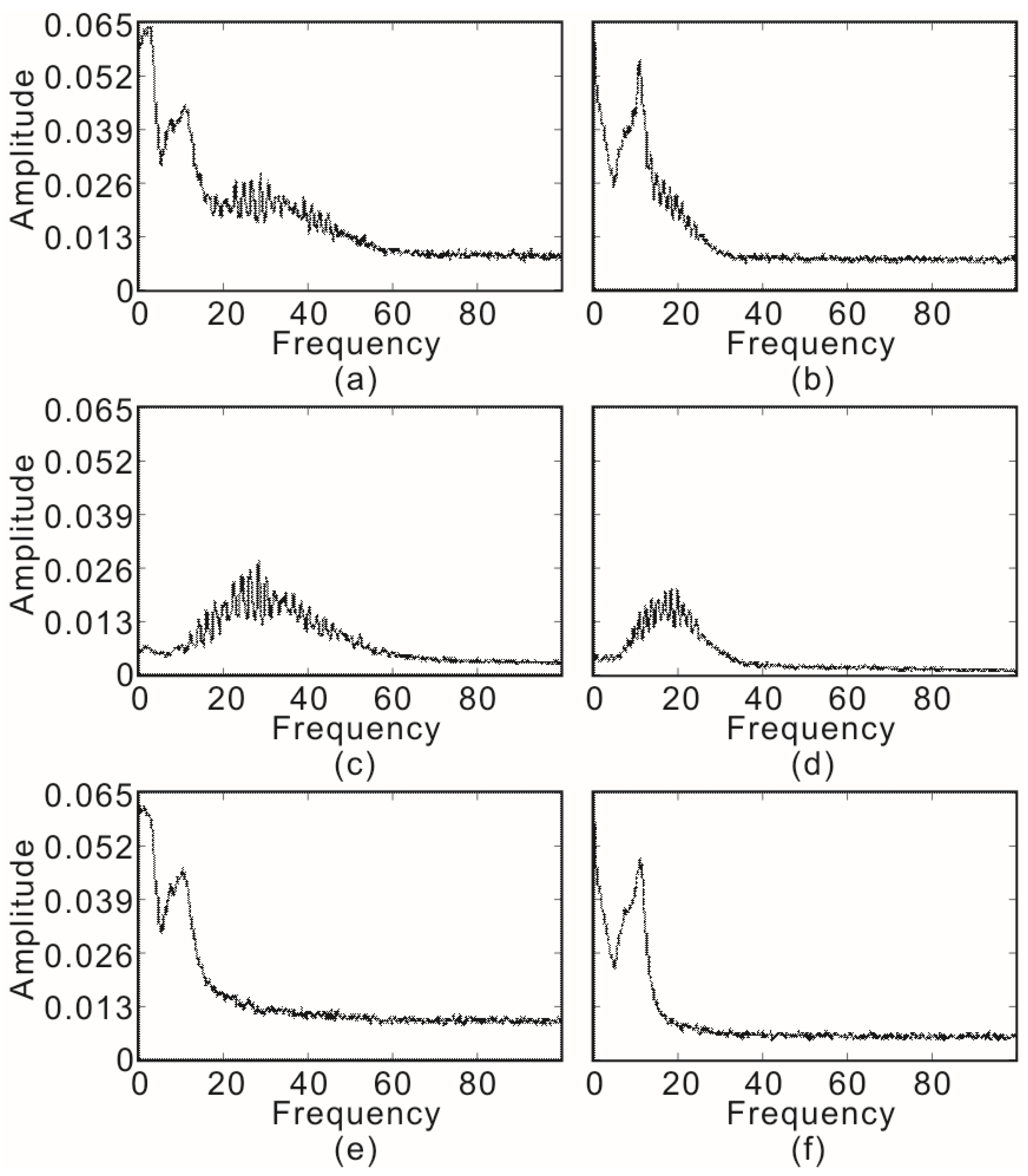
As displayed in Figure 13, the both valid PP- and PS-waves are effectively separated from their noisy backgrounds. From Figure 13c,d, it is clear that our noise attenuation method does not damage the valid waves. As seen in the frequency spectra shown in Figure 14a,b, before applying our filtering method, ground roll dominates the signal energy while the background random noise is spread out over the high-frequency area of the spectrum. However, as shown in Figure 14c–f, our filtering method effectively recovers the frequency spectra of the PP- and PS-reflections without damaging their low- and high-frequency energy parts.

3.3. Comparison with Instantaneous Polarization Filtering

We compare our approach with the instantaneous polarization filtering method based on complex trace analysis. Using the Hilbert transform, we get 2C analytical seismic signals X(t) and Z(t) as:

$$\{\begin{array}{l}X\left(t\right)=x_r\left(t\right)+i{x}_q\left(t\right)\\ Z\left(t\right)=z_r\left(t\right)+i{z}_q\left(t\right)\end{array}$$

(19)

where x_r(t) and z_r(t) are the real X- and Z-component data, and x_q(t) and z_q(t) are the Hilbert transforms of x_r(t) and z_r(t), respectively. From René et al., we obtain the squares of the semi-major and semi-minor axis lengths as, respectively [33],

$$\{\begin{array}{l}{a}^2\left(t\right)=\left\{S_0\left(t\right)+{\left[S_1^2\left(t\right)+S_2^2\left(t\right)\right]}^{\frac{1}{2}}\right\}/2\\ b^2\left(t\right)=\left\{S_0\left(t\right)-{\left[S_1^2\left(t\right)+S_2^2\left(t\right)\right]}^{\frac{1}{2}}\right\}/2\end{array}$$

(20)

where

$$\{\begin{array}{l}{S}_0\left(t\right)={\left|Z\left(t\right)\right|}^2+{\left|X\left(t\right)\right|}^2\\ S_1\left(t\right)={\left|Z\left(t\right)\right|}^2-{\left|X\left(t\right)\right|}^2\\ S_2\left(t\right)=2\left|Z\left(t\right)\right|\left|X\left(t\right)\right|\cos \left(\arctan \frac{x_r\left(t\right)z_q\left(t\right)-z_r\left(t\right)x_q\left(t\right)}{z_r\left(t\right)x_r\left(t\right)+z_q\left(t\right)x_q\left(t\right)}\right)\end{array}$$

(21)

Then, the instantaneous reciprocal ellipticity and tilt angle are given by, respectively,

$$\{\begin{array}{l}e\left(t\right)=\frac{b\left(t\right)}{a\left(t\right)}\\ \theta \left(t\right)=\left(\arctan \frac{S_2\left(t\right)}{S_1\left(t\right)}\right)/2\end{array}$$

(22)

Following the method proposed by Perelberg and Hornbostel [4], a separated valid signal may be defined as:

$$R\left(t\right)=G_1\left(t\right)G_2\left(t\right)S\left(t\right)$$

(23)

where S(t) is the input data for X(t) or Z(t), and G₁(t) and G₂(t) are the weighting functions based on the ellipticity and tilt angle, respectively, and

$$G_1\left(t\right)=\exp \left(-{\left(1-e\left(t\right)\right)}^2/2{\sigma }_e^2\right)$$

(24)

$$G_2\left(t\right)=\exp \left(-\Delta \theta {\left(t\right)}^2/2{\sigma }_{\theta }^2\right)$$

(25)

where Δθ is the angular difference between the actual tilt angle and desired tilt angle and σ_e and σ_θ are the standard deviations of ellipticity and tilt angle, respectively.

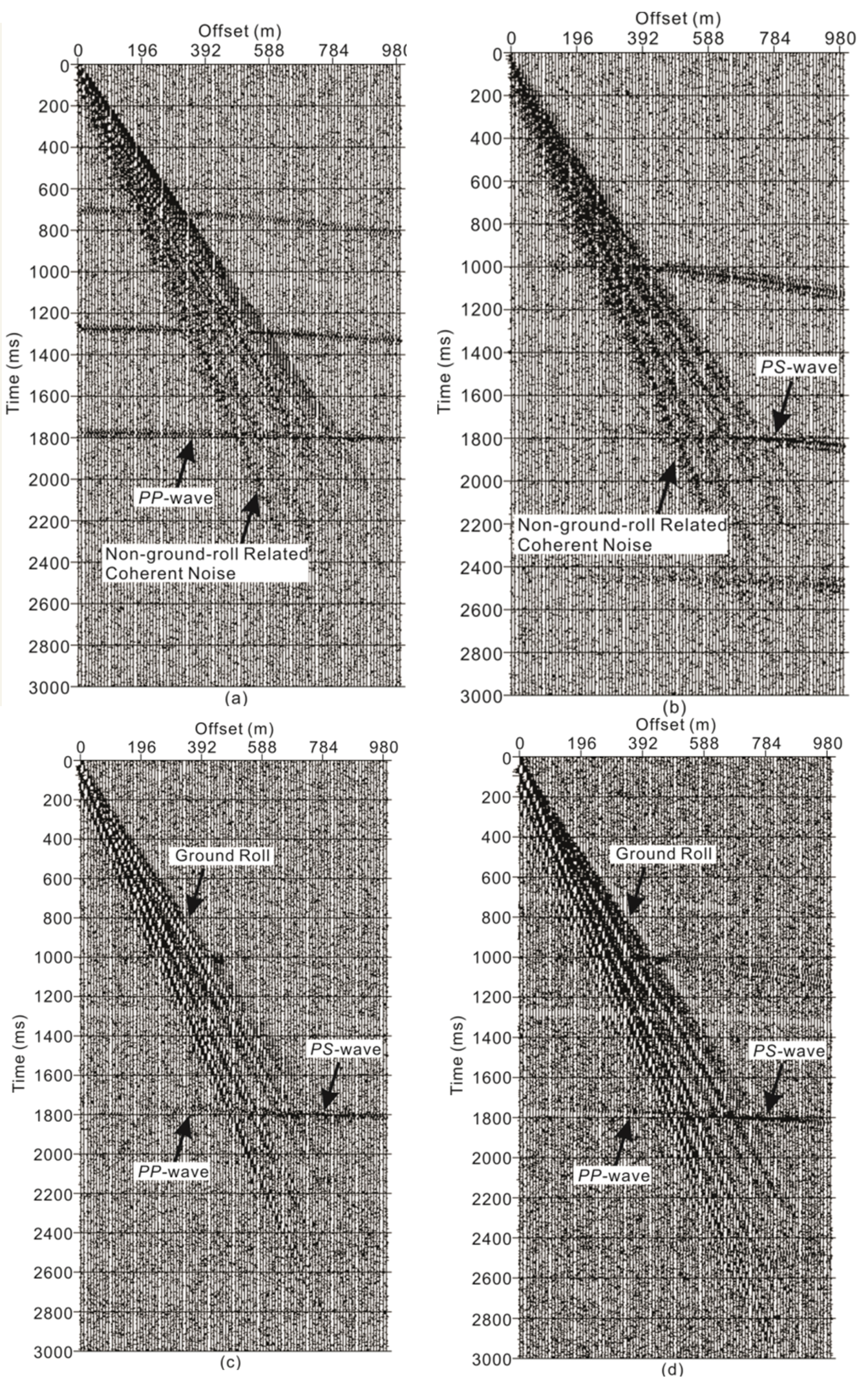
As shown in Figure 15, the instantaneous polarization filtering method can effectively filter out the ground roll. However, the instantaneous polarization filtering method relies on the polarization difference between body waves and noise. Therefore, if the polarization trajectory of a body wave is close to the ground roll, the performance of the instantaneous polarization filtering method declines. For example, the PP- and PS-reflections near 1800 ms (Figure 15c,d) are damaged to some extent because they are interfered together and exhibited similar polarization characteristics as the ground roll. Moreover, the non-ground-roll related coherent noise and random noise are not adequately suppressed (Figure 15a,b). The correlation coefficients between the filtered Z- and X-components (Figure 13a,b) derived by the proposed method and the noise-free Z- and X-components are 0.804 and 0.839, respectively. Nevertheless, those between the filtered Z- and X-components (Figure 15a,b) derived with the instantaneous polarization filtering and the noise-free Z- and X-components are 0.124 and 0.246, respectively. Compared with Figure 13, it is obvious that our noise attenuation method is more powerful in the discrimination of body waves from a noisy background.

4. Application Results and Discussion

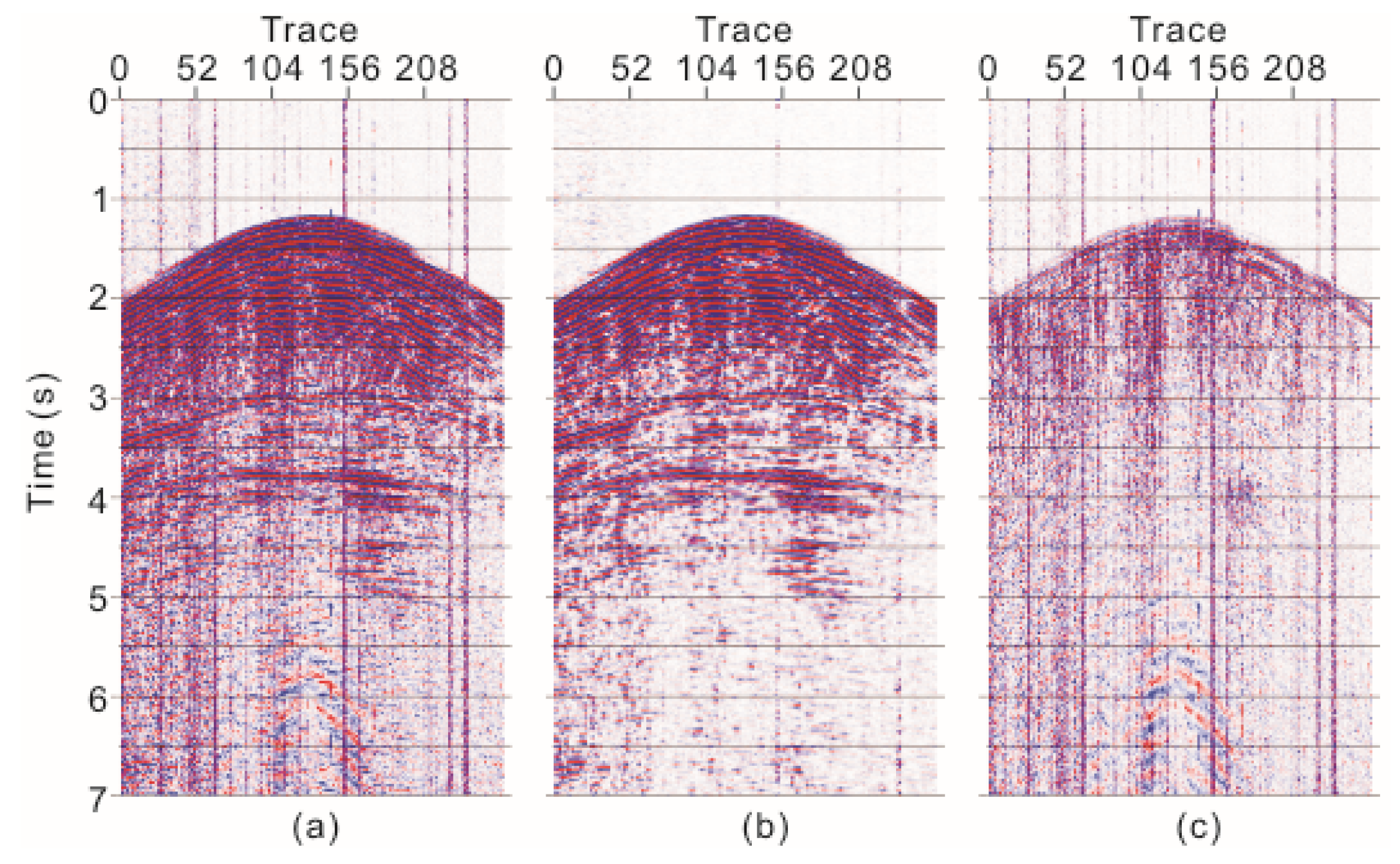
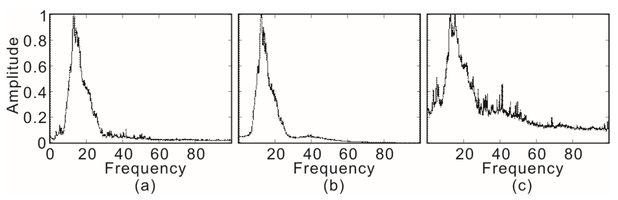
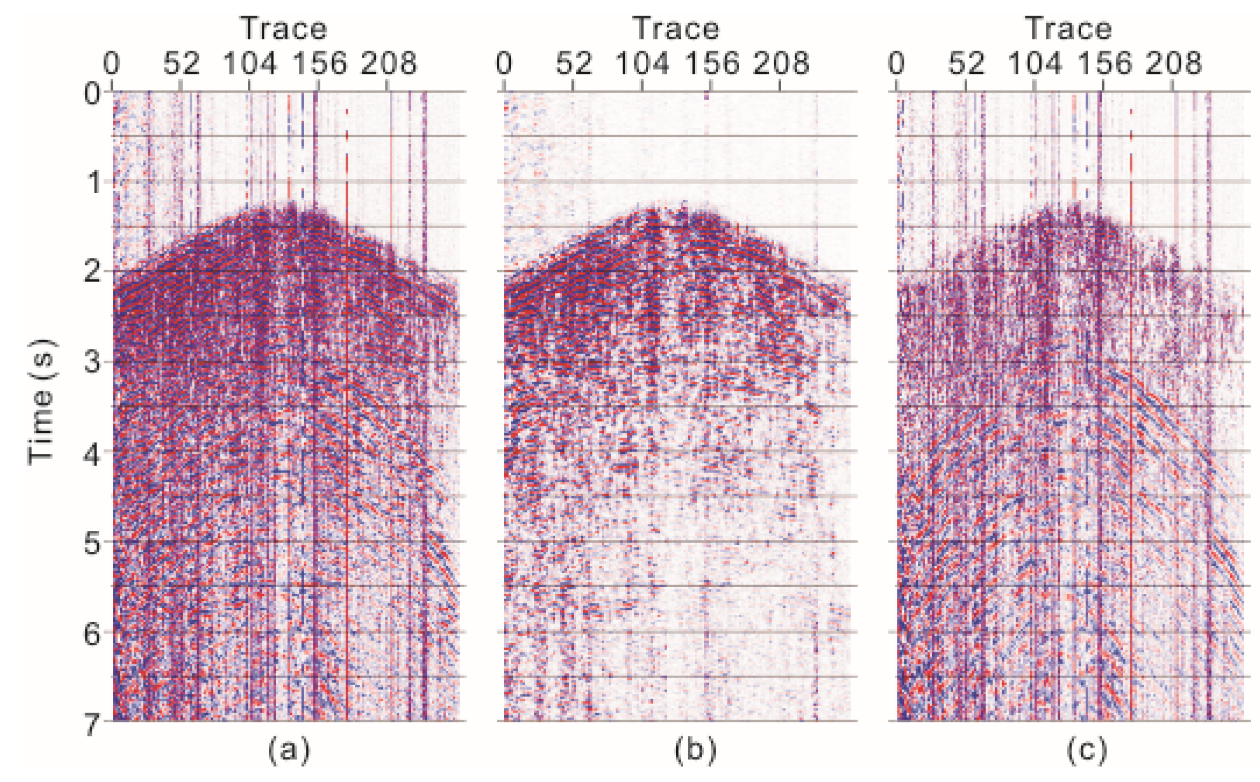
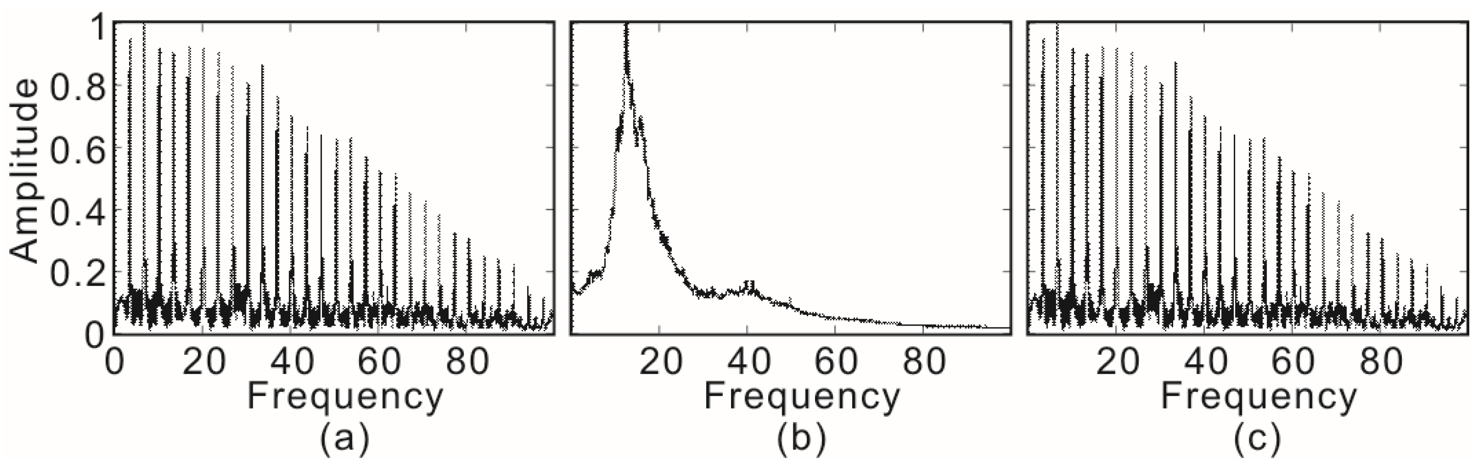
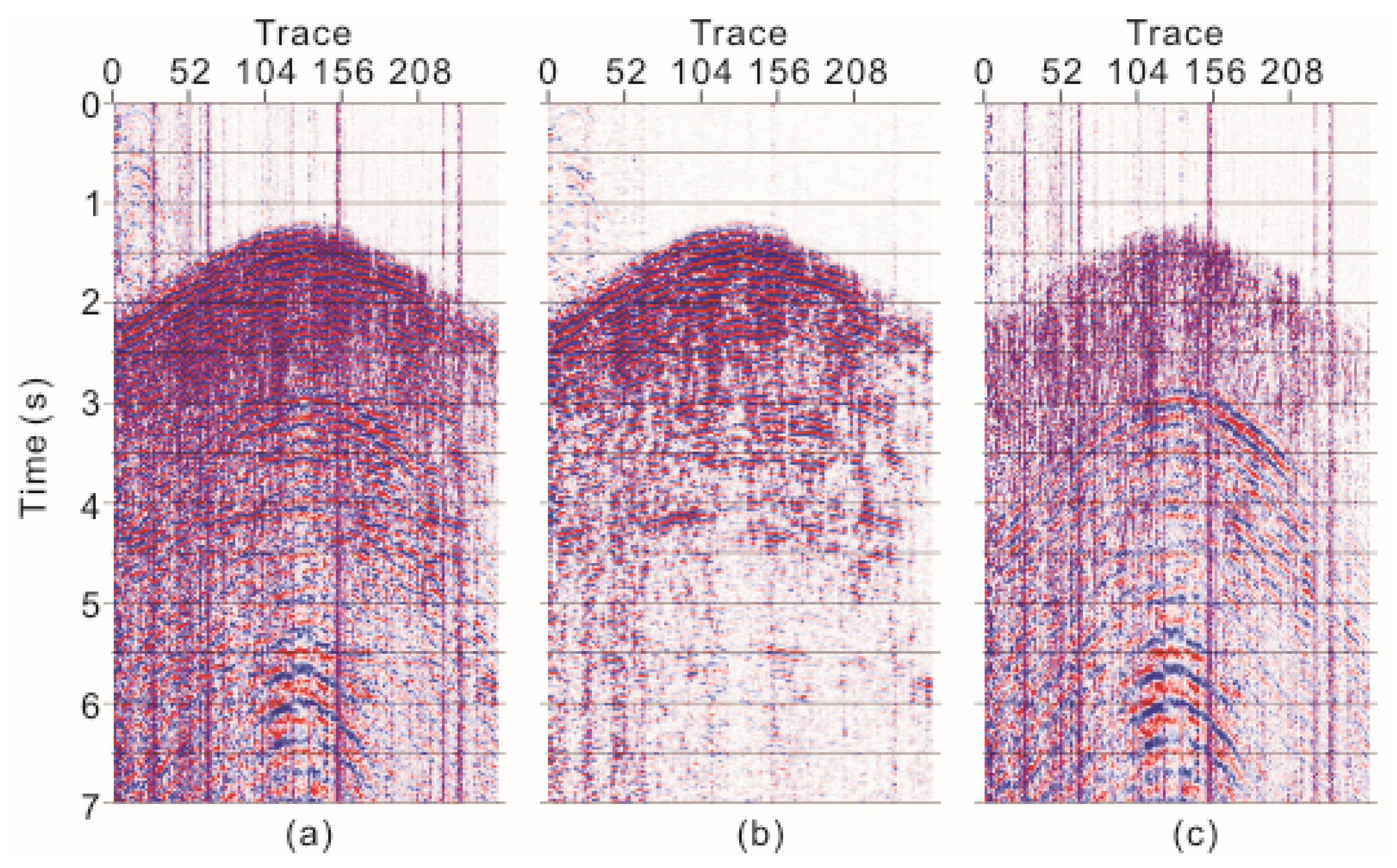
We apply our noise attenuation method to field three-dimensional three-component data acquired from the Xinchang gas field in the Sichuan Basin, Southwest China. The adopted moving window for the suppression of ground roll is 70 ms and that for the suppression of non-ground-roll related noise and random noise is 5-trace and 9 ms. Our method can greatly suppress ground roll, random noise, and other strong coherent noise from the Z-component (Figure 16); the removed noise is mainly of a wide frequency-band (Figure 17). However, the first arrivals on the Z-component are also removed, which cause the frequency energy of the seismic primary to occur on the Z-component frequency spectrum (Figure 17c). On the X-component (Figure 18 and Figure 19), in addition to ground roll and random noise, noises such as outliers and single frequency interferences are also adequately suppressed. Satisfied filtering results are also found on the T-component (Figure 20 and Figure 21). Overall, our noise attenuation method greatly improves the S/N of the field multicomponent data, while also maintaining valid signal amplitudes.

Our noise attenuation method is based on the wave vector characteristics of elastic wavefields on all components. The method requires that previous data-processing procedures have not changed the relative amplitude relationships among different components. For example, in bandpass filtering, amplitude scaling, or static correction, all processing parameters for all components should be consistent. Deconvolution should not be performed before using our method, because it will change the shape of the wavelet on different components. Horizontal rotation (R-T rotation) will not change the vector amplitudes of elastic wavefields [1], so our method can be implemented before or after horizontal rotation. In this application, the proposed method is implemented before horizontal rotation and the only processing is the exponential gain of the three components on the same scale.

In order to ensure the robustness of the algorithm in the proposed method, the sampling rate, recording length, and trace number of each input component are required to be the same. The key loops of the algorithm totally take M × N × (L1 + L2 + L3) iterations (M: trace number, N: sample number, L1: moving sample number for suppressing ground roll, L2: moving sample number for suppressing random noise, L3: moving trace number for suppressing non-ground-roll related coherent noise). In addition, the seismic data are not required to be transformed into another domain. Therefore, the proposed method is economical in terms of computational cost.

Our noise attenuation method is implemented within some certain sizes of moving windows. One moving-time-window size should be close to the maximum apparent period of the valid signal for suppressing ground roll. If the absorption attenuation is serious, the apparent period of the valid signal will increase with time. Then, at different times, we can extract several valid signals to estimate time-variant moving window sizes. In addition, the moving time window for the calculation of ground-roll vectors often results in shallow refractions and wide-angle reflections for strong vector amplitudes. Therefore, it is necessary to set a filtering area for the input data when suppressing ground roll.

The other moving-time-window size should be calculated based on the high-cutoff frequency of the valid signal to suppress random noise. Similarly, we can determine the corresponding time-variant moving window sizes based on the valid signals extracted at different times. In addition, a small moving time window for random noise attenuation can also lead to large vector amplitudes of shallow refractions and wide-angle reflections. The field application shows that some shallow refractions and wide-angle reflections are filtered, especially on the Z-component. Nevertheless, this does not affect the applicability of our noise attenuation method.

Near the start and end times of a 3C dataset, the filtering effect will be worse owing to the insufficient size of the moving time window. In addition, a similar phenomenon will occur near the start trace and end trace within a receiving line. To make up for this deficiency, we can extend the border of the filtering window used for suppressing ground roll wider. Finally, our noise attenuation method is applicable if the non-ground-roll related coherent noise covers continuous multiple seismic traces, because a large moving trace window is required, which will also greatly damage the valid signal.

The proposed method is applicable for the noise attenuation of the land two- or three-component seismic data and the three-component ocean bottom seismic data. To the borehole multi-component seismic data, the suppression of interference waves, such as tube waves and multiples, is one of the main problems. Thus, noise attenuation based on the wave vector characteristics for the borehole multi-component seismic data will require further detailed study.

5. Conclusions

We have developed a noise attenuation method based on wave vector characteristics. The key part of our method is the discrimination of polarizations of valid seismic signals and noise based mean (or median) wave vectors. In our method, the wave vectors of ground roll, valid signal, random noise and non-ground-roll related coherent noise in 3C records are separated through the smoothing of wave vectors with different moving window sizes and directions. Generally, the moving-time-window sizes adopted to suppress ground roll and random noise should be close to the maximum apparent period and half of the reciprocal of high-cutoff frequency of the valid signal, respectively. Our noise attenuation can be applied to both land and ocean bottom multi-component records. Specially, the ground roll received on the Y-component can also be filtered out, although ground roll is often assumed to be polarised on a two-dimensional vertical plane. Meanwhile, 2C or 3C records together can help to discriminate the spatial particle motion of body waves from a noisy background. Tests show that our noise attenuation method is effective for both numerical and field data applications and the effect of the proposed method is better than that of the instantaneous polarization filter. This method will be useful for obtaining pure elastic wavefields in multi-component seismic surveys.

References

- Gaiser, J.E. Applications for vector coordinate systems of 3-D converted-wave data. Lead. Edge 1999, 18, 1290–1300. [Google Scholar] [CrossRef]
- Kishore, S.A.; Prosenjit, D.; Sastry, M.H.; Tewari, S.K.; Baloni, C.L. 3D-3C Seismic data acquisition—Survey design and implementation: A case study NAS Block, A & AA Basin. In Proceedings of the 9th Biennial International Conference & Exposition on Petroleum Geophysics, Hyderabad, India, 16–18 February 2012; pp. 260–264. [Google Scholar]
- Schimmel, M.; Gallart, J. Degree of polarization filter for frequency-dependent signal enhancement through noise suppression. Bull. Seismol. Soc. Am. 2004, 94, 1016–1035. [Google Scholar] [CrossRef]
- Perelberg, A.I.; Hornbostel, S.C. Applications of seismic polarization analysis. Geophysics 1994, 59, 119–130. [Google Scholar] [CrossRef]
- Schimmel, M.; Gallart, J. The use of instantaneous polarization attributes for seismic signal detection and image enhancement. Geophys. J. Int. 2003, 155, 653–668. [Google Scholar] [CrossRef]
- Flinn, E.A. Signal analysis using rectilinearity and direction of particle motion. Proc. IEEE 1965, 53, 1874–1876. [Google Scholar] [CrossRef]
- Montalbetti, J.F.; Kanasewich, E.R. Enhancement of teleseismic body phases with a polarization filter. Geophys. J. Int. 1970, 21, 119–129. [Google Scholar] [CrossRef]
- Kanasewich, E.R. Time Sequence Analysis in Geophysics, 3rd ed.; University of Alberta Press: Edmonton, AB, Canada, 1981. [Google Scholar]
- Vidale, J.E. Complex polarization analysis of particle motion. Bull. Seismol. Soc. Am. 1986, 76, 1393–1405. [Google Scholar]
- Du, Z.; Foulger, G.R.; Mao, W. Noise reduction for broad-band, three-component seismograms using data-adaptive polarization filters. Geophys. J. Int. 2000, 141, 820–828. [Google Scholar] [CrossRef]
- Kulesh, M.; Diallo, M.S.; Holschneider, M.; Kurennaya, K.; Krüger, F.; Ohrnberger, M.; Scherbaum, F. Polarization analysis in the wavelet domain based on the adaptive covariance method. Geophys. J. Int. 2007, 170, 667–678. [Google Scholar] [CrossRef]
- Benhama, A.; Cliet, C.; Dubesset, M. Study and applications of spatial directional filtering in three-component recordings. Geophys. Prospect. 1988, 36, 591–613. [Google Scholar] [CrossRef]
- Shieh, C.-F.; Herrmann, R.B. Ground roll: Rejection using polarization filters. Geophysics 1990, 55, 1216–1222. [Google Scholar] [CrossRef]
- Kragh, E.; Peardon, L. Ground roll and polarization. First Break 1995, 13, 369–378. [Google Scholar] [CrossRef]
- De Franko, R.; Musacchio, G. Polarization filter with singular value decomposition. Geophysics 2001, 66, 932–938. [Google Scholar] [CrossRef]
- Tiapkina, O.; Landrø, M.; Tyapkin, Y.; Link, B. Single-station SVD-based polarization filtering of ground roll: Perfection and investigation of limitations and pitfalls. Geophysics 2012, 77, V41–V59. [Google Scholar] [CrossRef]
- Samson, J.C. The spectral matrix, eigenvalues, and principal components in the analysis of multichannel geophysical data. Ann. Geophys. 1983, 1, 115–119. [Google Scholar]
- Park, J.; Vernon, F.L., III; Lindberg, C.R. Frequency dependent polarization analysis of high-frequency seismograms. J. Geophys. Res. 1987, 92, 12664–12674. [Google Scholar] [CrossRef]
- Jurkevics, A. Polarization analysis of three-component array data. Bull. Seismol. Soc. Am. 1988, 78, 1725–1743. [Google Scholar]
- Morozov, I.B.; Smithson, S.B. Instantaneous polarization attributes and directional filtering. Geophysics 1996, 61, 872–881. [Google Scholar] [CrossRef]
- Diallo, M.S.; Kulesh, M.; Holschneider, M.; Scherbaum, F. Instantaneous polarization attributes in the time-frequency domain and wavefield separation. Geophys. Prospect. 2005, 53, 723–731. [Google Scholar] [CrossRef]
- Diallo, M.S.; Kulesh, M.; Holschneider, M.; Kurennaya, K.; Scherbaum, F. Instantaneous polarization attributes based on an adaptive approximate covariance method. Geophysics 2006, 71, V99–V104. [Google Scholar] [CrossRef]
- Diallo, M.S.; Kulesh, M.; Holschneider, M.; Scherbaum, F.; Adler, F. Characterization of polarization attributes of seismic waves using continuous wavelet transforms. Geophysics 2006, 71, V67–V77. [Google Scholar] [CrossRef]
- Lu, J.; Wang, Y.; Yang, C.Y. Instantaneous polarization filtering focused on suppression of surface waves. Appl. Geophys. 2010, 7, 88–97. [Google Scholar] [CrossRef]
- Diallo, M.S.; Ross, W.S.; Shatilo, A.P.; Dura-Gomez, I.; Szurek, G.C. Application of constrained polarization filtering for surface-wave mitigation: Three case studies. Geophysics 2012, 77, V169–V181. [Google Scholar] [CrossRef]
- Hou, S.; Luo, Y.; Kelamis, P.G. Simultaneous sources separation via multidirectional vector-median filtering. Geophysics 2012, 77, V123–V131. [Google Scholar]
- Liu, Y. Noise reduction by vector median filtering. Geophysics 2013, 78, V79–V86. [Google Scholar] [CrossRef]
- Al-Dossary, S.; Marfurt, K.J. Lineament-preserving filtering. Geophysics 2007, 72, P1–P8. [Google Scholar] [CrossRef]
- Lu, J.; Wang, Y.; Yang, Y.; Chen, J. Pre-stack separation of PP and split PS waves in HTI media. Geophys. J. Int. 2017, 210, 510–524. [Google Scholar] [CrossRef]
- Knopoff, L. A matrix method for elastic wave problems. Bull. Seismol. Soc. Am. 1964, 54, 431–438. [Google Scholar]
- Schwab, F.; Knopoff, L. Surface-wave dispersion computations. Bull. Seismol. Soc. Am. 1970, 60, 321–344. [Google Scholar]
- Mao, W.; Stuart, G.M. Rapid multi-wave-type ray tracing in complex 2-D and 3-D isotropic media. Geophysics 1997, 62, 298–308. [Google Scholar] [CrossRef]
- René, R.M.; Fitter, J.L.; Forsyth, P.M.; Kim, K.Y.; Murray, D.J.; Walters, J.K.; Westerman, J.D. Multicomponent seismic studies using complex trace analysis. Geophysics 1986, 51, 1235–1251. [Google Scholar] [CrossRef]
Figure 1.
Sketch map of mean wave vector set in a 3D space. The green vector is the median vector as defined by Equation (7).
Figure 2.
Wavelet plots: (a) valid signal and (b) its frequency spectrum.
Figure 3.
Moving windows used in median filtering to the wave vectors from shot three-component (3C) records. The red dots are seismic samples. The blue rectangles mark the moving windows for the median filtering performed over time. The green rectangle marks the moving windows for the median filtering performed over trace within the same receiving line.
Figure 4.
Synthetic two-component records. (a) Full two-component record; (b) the valid seismic signal at a 30 Hz dominant frequency; (c) the 50% random noise and (d) the ground roll.
Figure 5.
Results of ground roll separation. (a) Separated ground roll and (b) valid signal with random noise.
Figure 6.
Hodogram plots of two-component records. (a) Raw two-component records; (b) separated ground roll without adopting any scaling factor and (c) separated ground roll using scaling factors.
Figure 7.
Results of random noise filtering. (a) Valid seismic signals after random noise attenuation and (b) the removed random noise.
Figure 8.
Hodogram plots of the ground-roll-attenuated signal. (a) Ground-roll-attenuated signal; (b) the unscaled valid signal after random noise attenuation; (c) the scaled valid signal after random noise attenuation and (d) the removed random noise.
Figure 9.
Dispersion curve of the simulated ground roll.
Figure 10.
Synthetic shot records. (a) Z-component with noise; (b) X-component with noise; (c) pure ground roll added to the Z-component; (d) pure ground roll added to the X-component; (e) non-ground-roll related coherent noise added to the Z-component; (f) and non-ground-roll related coherent noise added to the X-component.
Figure 11.
Wave vector moduli calculated from the raw synthetic shot records. Moving time widow of (a) 50 ms, (b) 60 ms, (c) 70 ms, and (d) 80 ms.
Figure 12.
Wave vector moduli calculated from the synthetic shot records after ground roll attenuation. Calculation using (a) a 3-trace and 5-ms moving window; (b) a 3-trace and 7-ms moving window; (c) a 5-trace and 7-ms moving window, and (d) a 9-trace and 9-ms moving window.
Figure 13.
Final filtered shot records. (a) The valid Z-component signal; (b) the valid R-component signal; (c) noise removed from the Z-component and (d) noise removed from the R-component.
Figure 14.
Frequency spectra of the synthetic shot records. (a) The raw Z-component; (b) the raw R-component, (c) the final filtered Z-component; (d) the final filtered R-component; (e) noise removed from the Z-component; and (f) noise removed from the R-component.
Figure 15.
Instantaneous polarization filtering results. (a) Filtered Z-component; (b) filtered R-component; (c) noise filtered out from the Z-component and (d) noise filtered out from the R-component.
Figure 16.
Field Z-component application results. (a) Original Z-component; (b) the filtered Z-component and (c) noise removed from the Z-component.
Figure 17.
Frequency spectra of field Z-component application results. (a) Original Z-component; (b) filtered Z-component and (c) noise removed from the Z-component.
Figure 18.
Field X-component application results. (a) Original X-component; (b) filtered X-component and (c) noise removed from the X-component.
Figure 19.
Frequency spectra of field X-component application results. (a) Original X-component; (b) filtered X-component and (c) noise removed from the X-component.
Figure 20.
Field Y-component application results. (a) Original Y-component; (b) filtered Y-component and (c) noise removed from the Y-component.
Figure 21.
Frequency spectra of field Y-component application results. (a) Original Y-component; (b) filtered Y-component and (c) noise removed from the Y-component.