Fault Diagnosis of Rotating Machinery Based on the Multiscale Local Projection Method and Diagonal Slice Spectrum


Abstract
:1. Introduction
2. Methodology
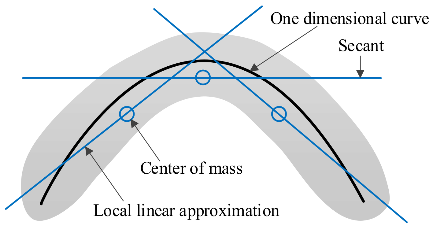
2.1. Standard Local Projection Algorithm
- (1)
- Choosing the appropriate parameters m and τ to reconstruct the noisy time series into the m-dimensional phase space.
- (2)
- Determine the neighborhood Un of each phase point. There are two methods to determine the neighborhood: the fixed neighborhood number and the fixed neighborhood radius. In this paper, the former is used.
- (3)
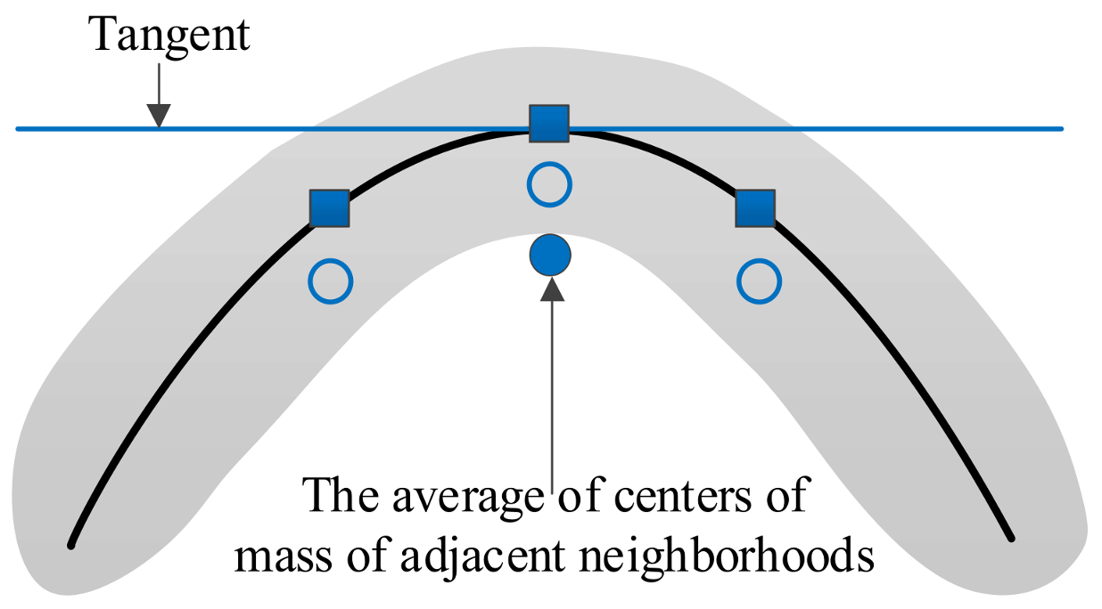
- Calculate the centroid of each neighborhood point.
- (4)
- The covariance matrix C of each phase point is calculated, and the eigenvalue decomposition is performed, and the eigenvalues corresponding to (m − m0) smaller eigenvalues aq (q = 1, 2, …, m − m0) are obtained.
- (5)
- Subtract the projection of the phase point on the noise subspace:where R is a diagonal weight matrix and is used to suppress the distortion of the elements at the beginning and end of the phase, in addition to keeping the elements stable in the middle. In this paper, R11 = Rmm = 103, and Rii = 1. is the centroid of the neighborhood, and is the signal after noise reduction.
- (6)
- Return to step (2) until all data have been processed.
2.2. Multiscale Local Projection Algorithm
2.3. The Basic Principle of Diagonal Slice Spectrum
- (1)
- If x(t) is a Gaussian signal, then its third-order cumulant diagonal slice spectrum Sx(w) = 0. This indicates that the diagonal slice spectrum can suppress Gaussian noise.
- (2)
- If the probability density function of x(t) obeys the symmetric distribution, its third-order cumulant diagonal slice spectrum Sx(w) = 0. This indicates that the diagonal slice spectrum can suppress the noise of symmetrical distribution.
- (3)
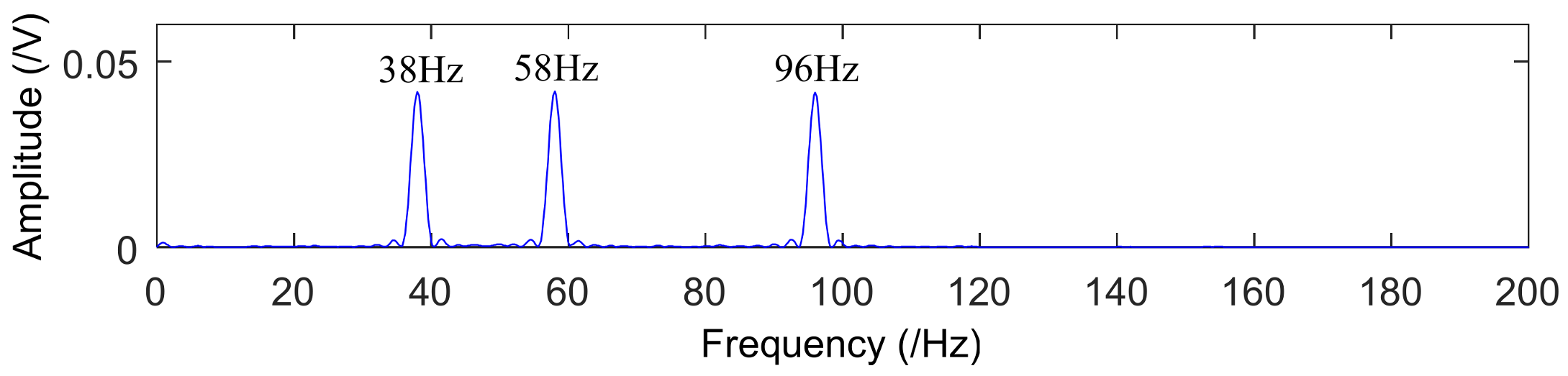
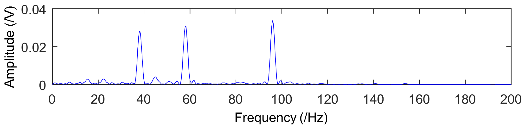
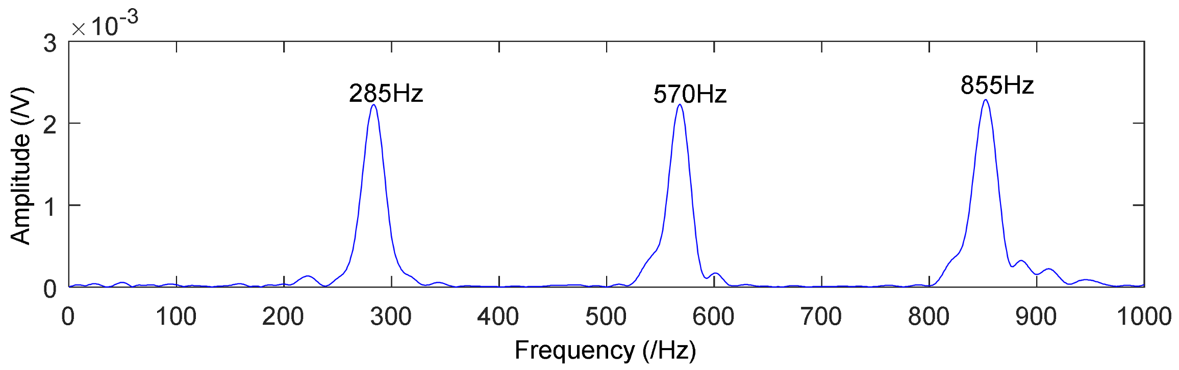
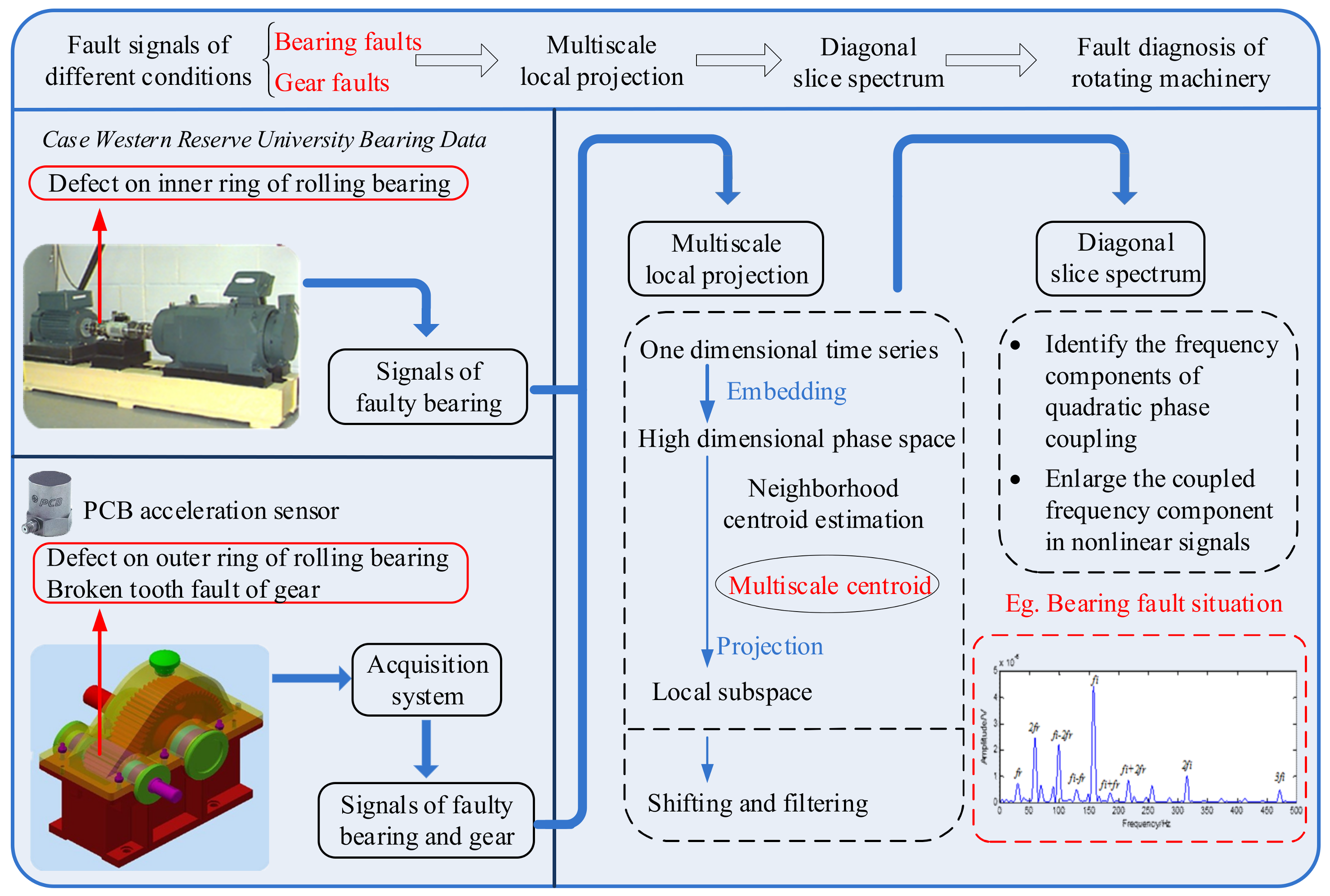
- If the harmonic signal has three components, the frequency and phase are respectively fk and φk (k = 1, 2, 3). Assuming f1 > f2 > f3, if both f1 = f2 + f3 and φ1 = φ2 + φ3 are satisfied, it can be concluded that the three harmonic components meet the secondary phase coupling relationship, and then Sx(w) = 0. Conversely, if these two conditions cannot meet simultaneously, then Sx(w) ≠ 0. This shows that the diagonal slice spectrum can identify the frequency components of quadratic phase coupling and enlarge the coupled frequency component in the nonlinear signal.
2.4. Feature Extraction Method of Mechanical Fault Based on Multiscale Local Projection Algorithm and Diagonal Slice Spectrum
3. Numerical Simulation
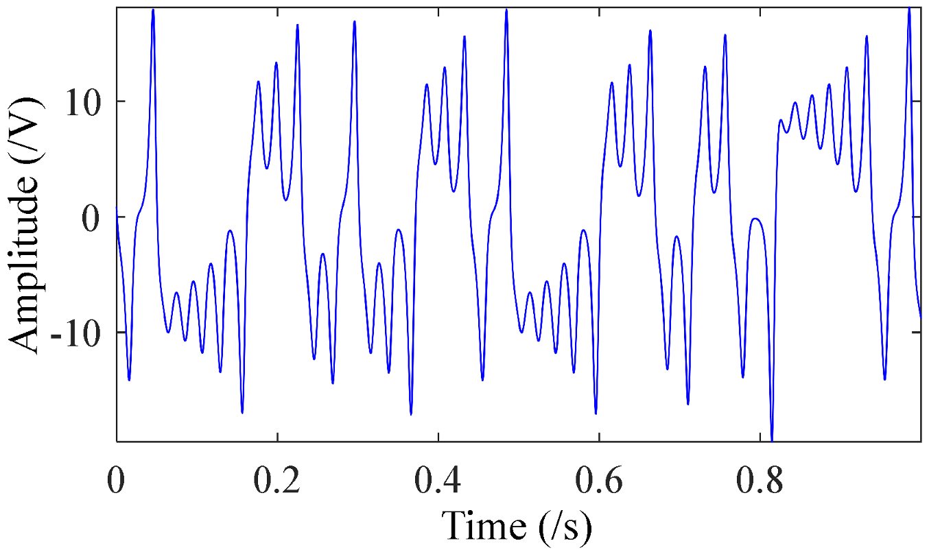
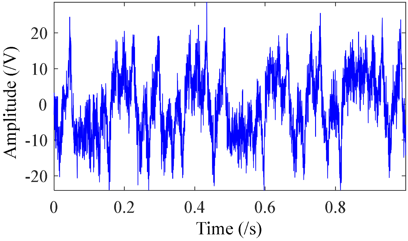
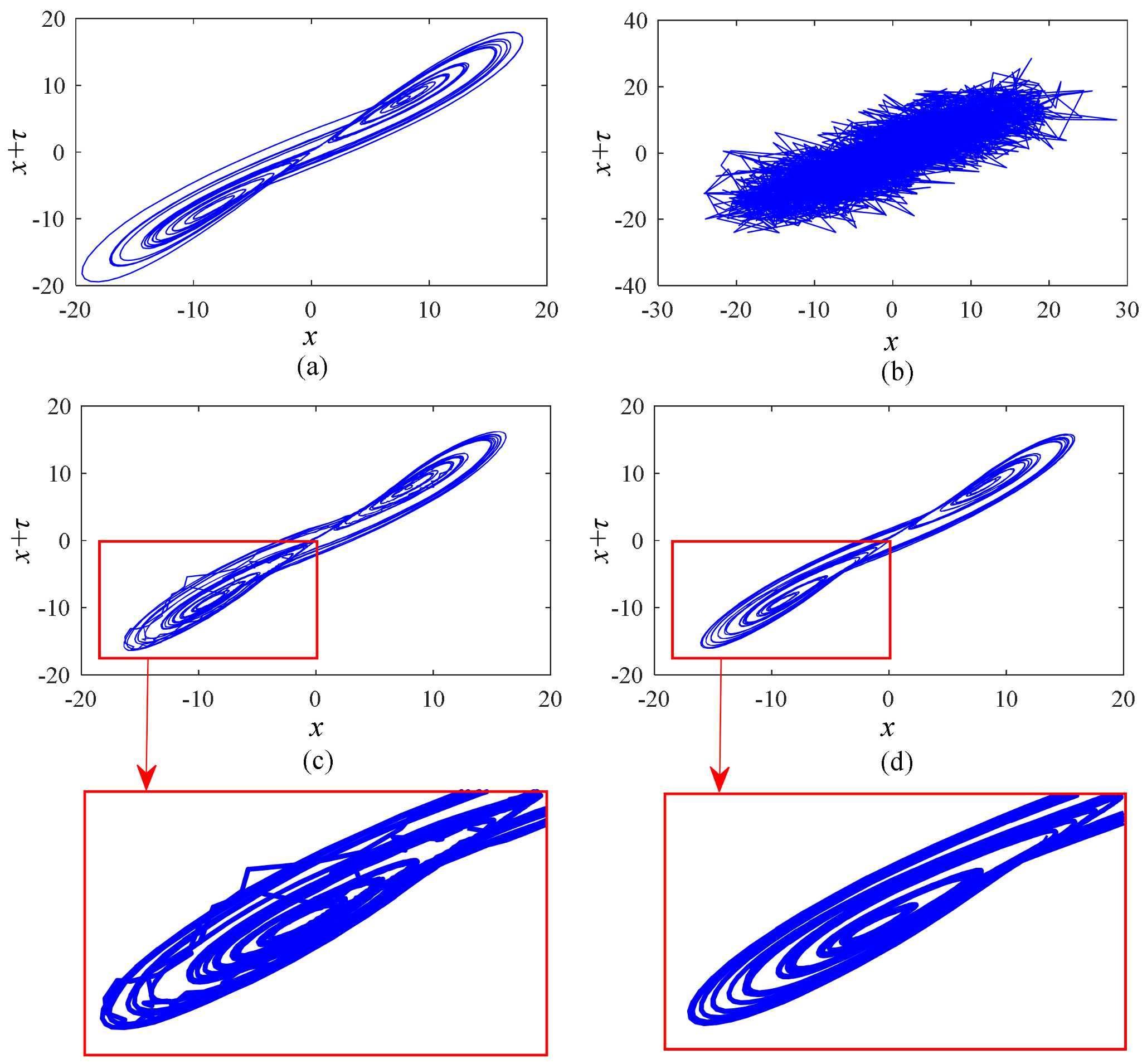
3.1. Numerical Simulation of Chaotic Signals
- (1)
- Mean Squared Error (MSE)
- (2)
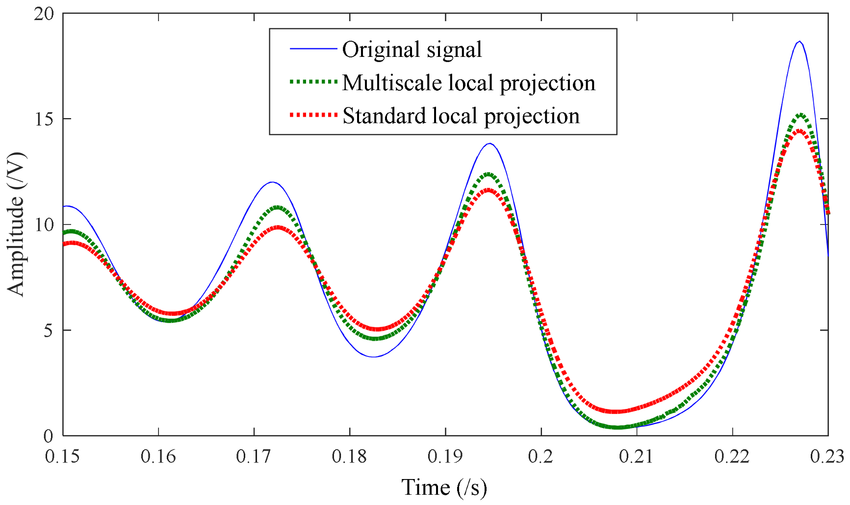
- Cross Correlation (CC)where x represents the original clean signal and represents the signal after noise reduction. A smaller MSE value means smaller deviation between the original signal and the denoised signal, and a bigger CC value means higher similarity between them. The evaluation results obtained by the above two algorithms are shown in Table 1. It can be concluded that the MSE value of the denoised signal obtained by multiscale local projection noise reduction is smaller, while the CC value is larger. It demonstrates that multiscale local projection has a better denoising effect than standard local projection.
3.2. Simulation of Diagonal Slice Spectrum
4. Fault Simulation Experiment of Rolling Bearing and Gear
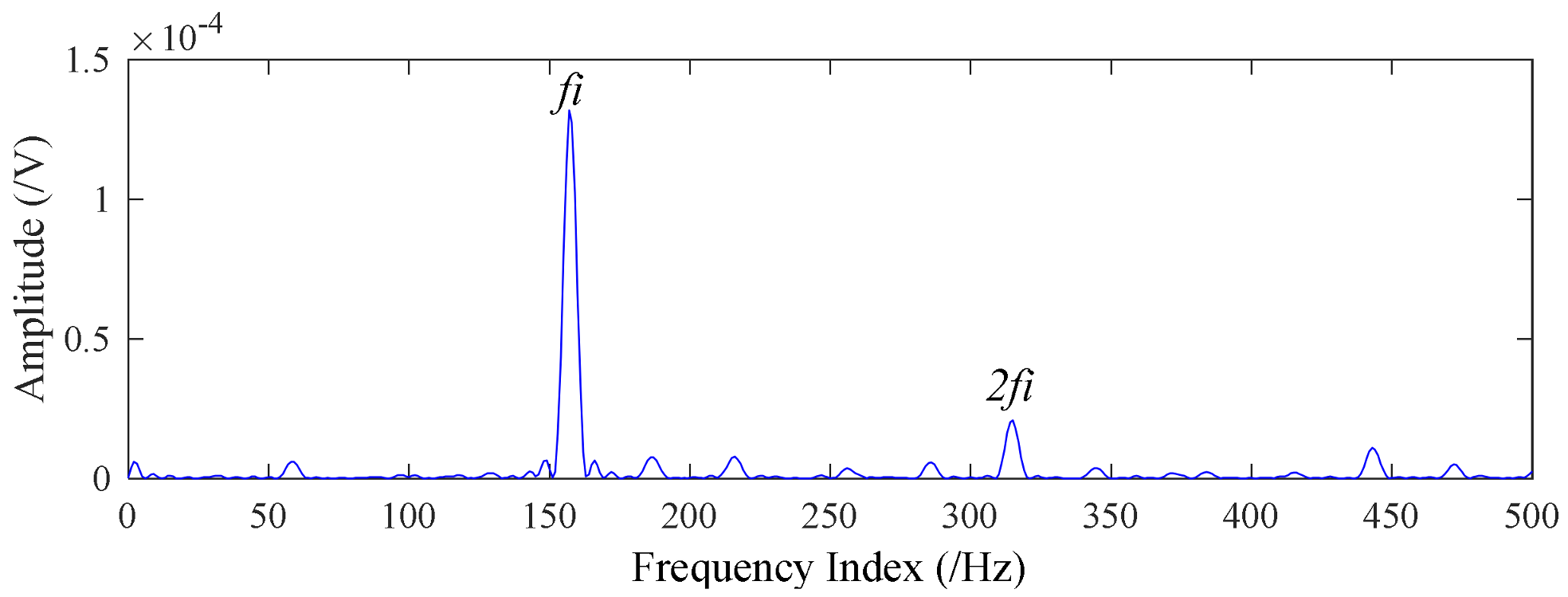
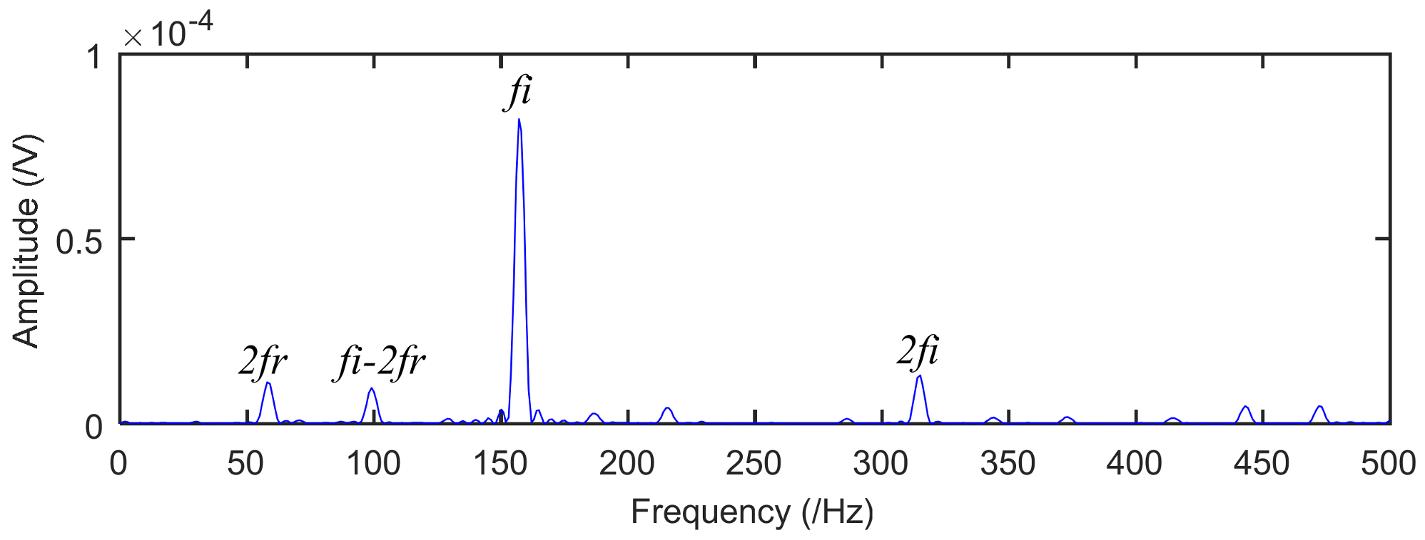
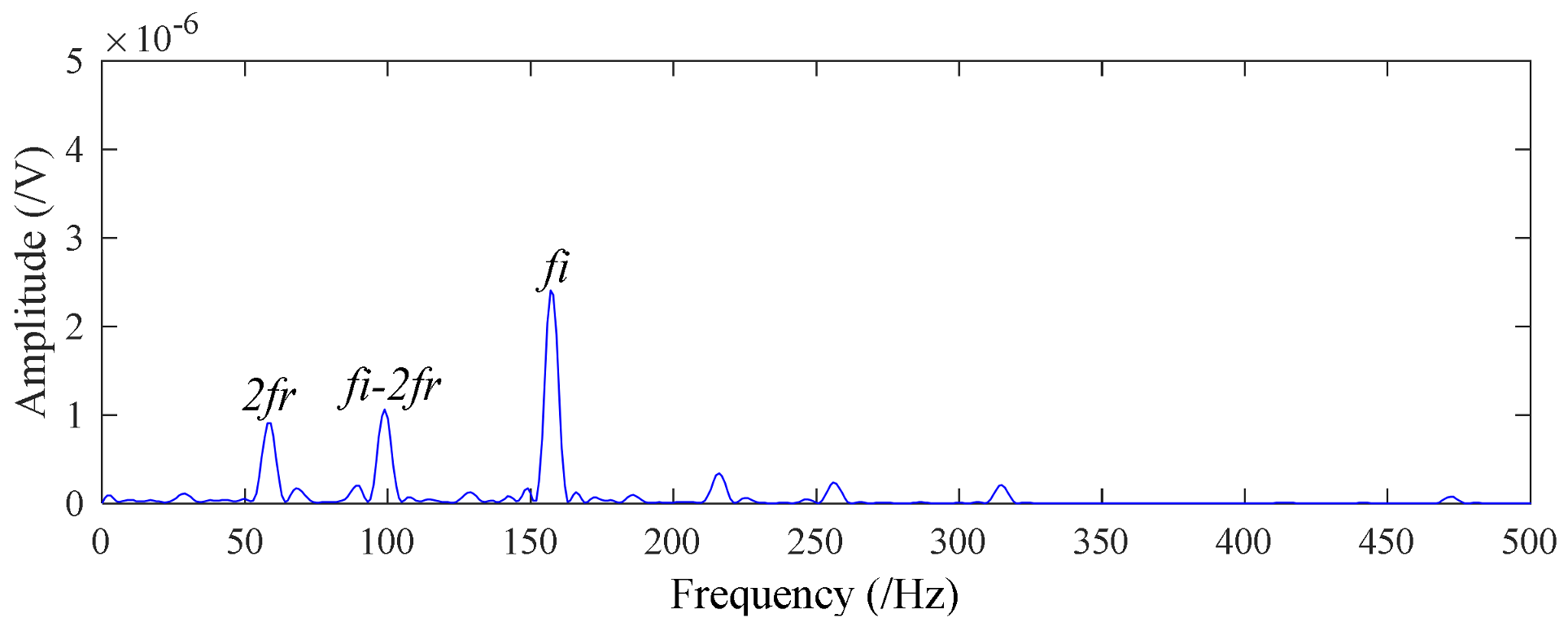
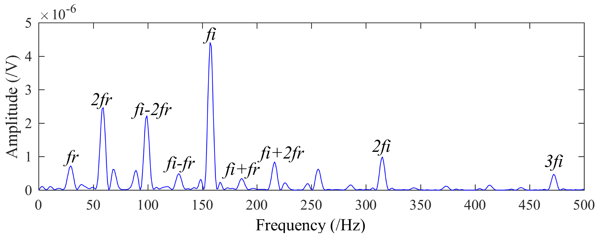
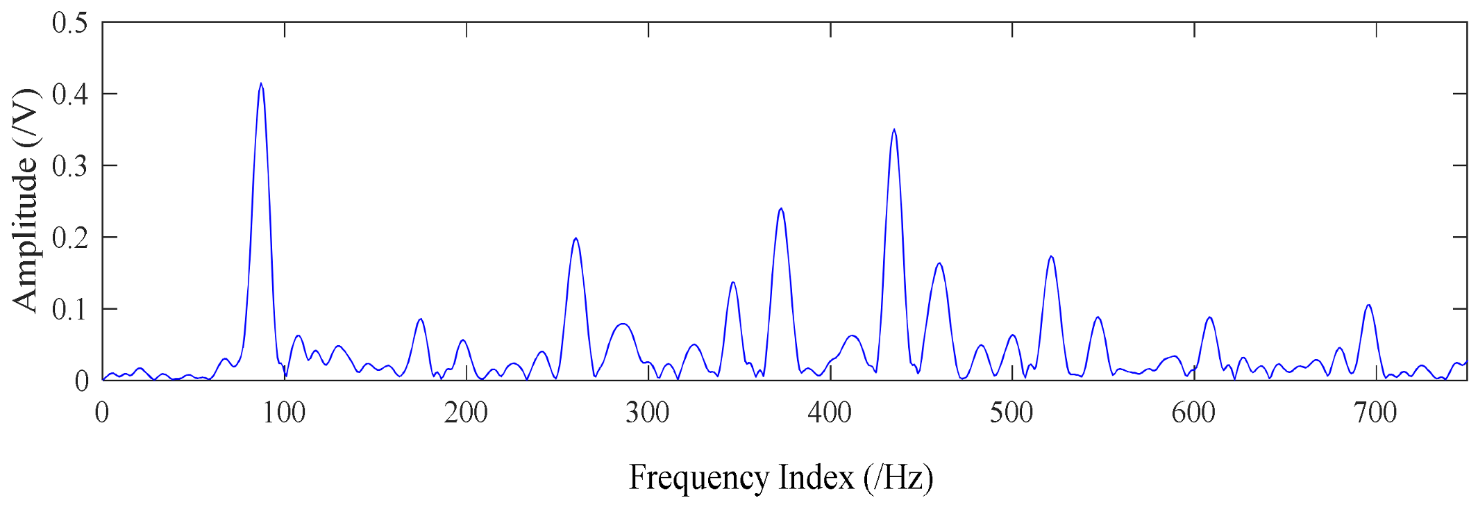
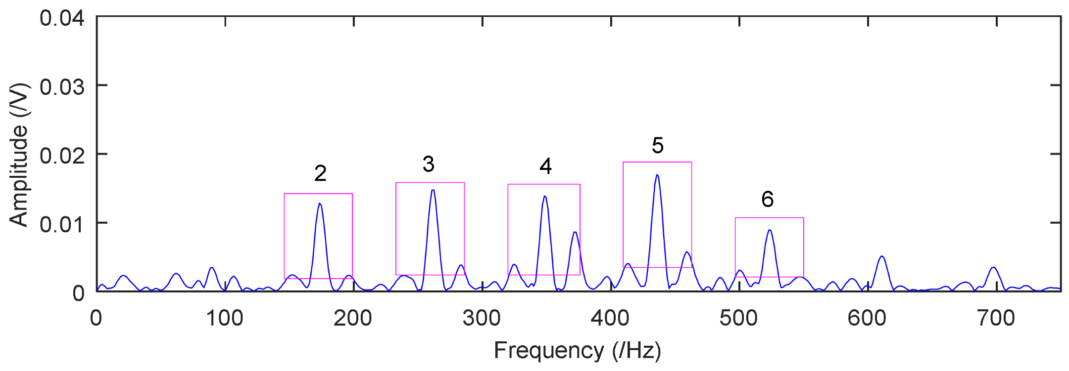
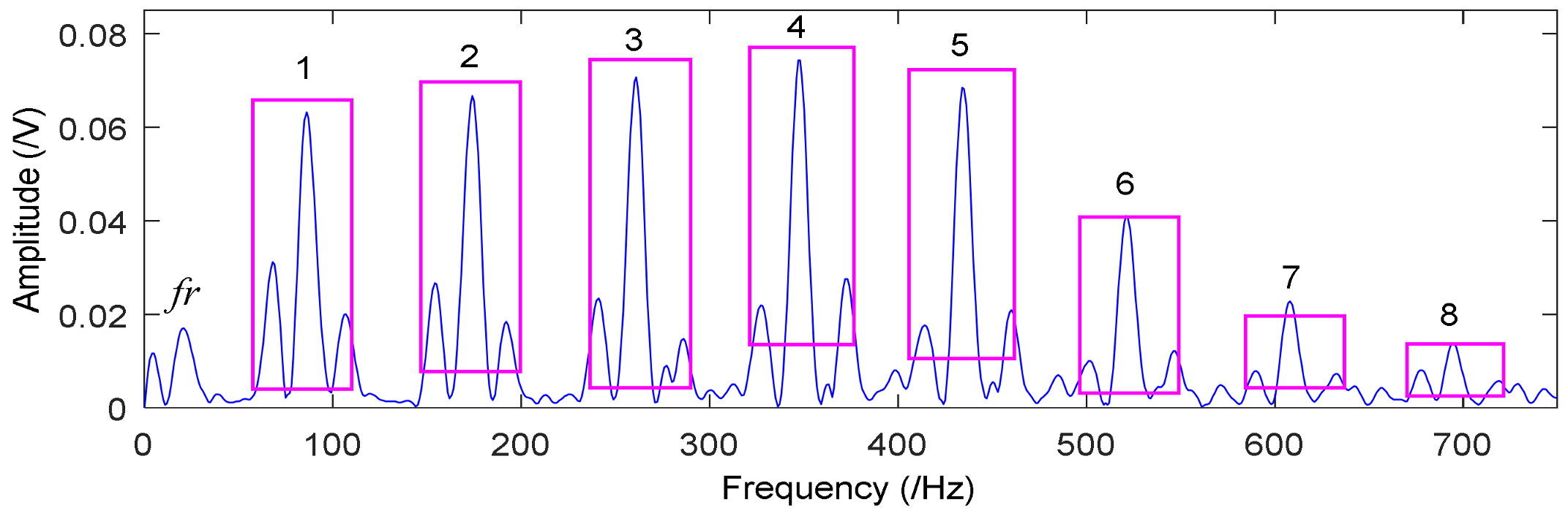
4.1. Application to Case Western Reserve University Bearing Data
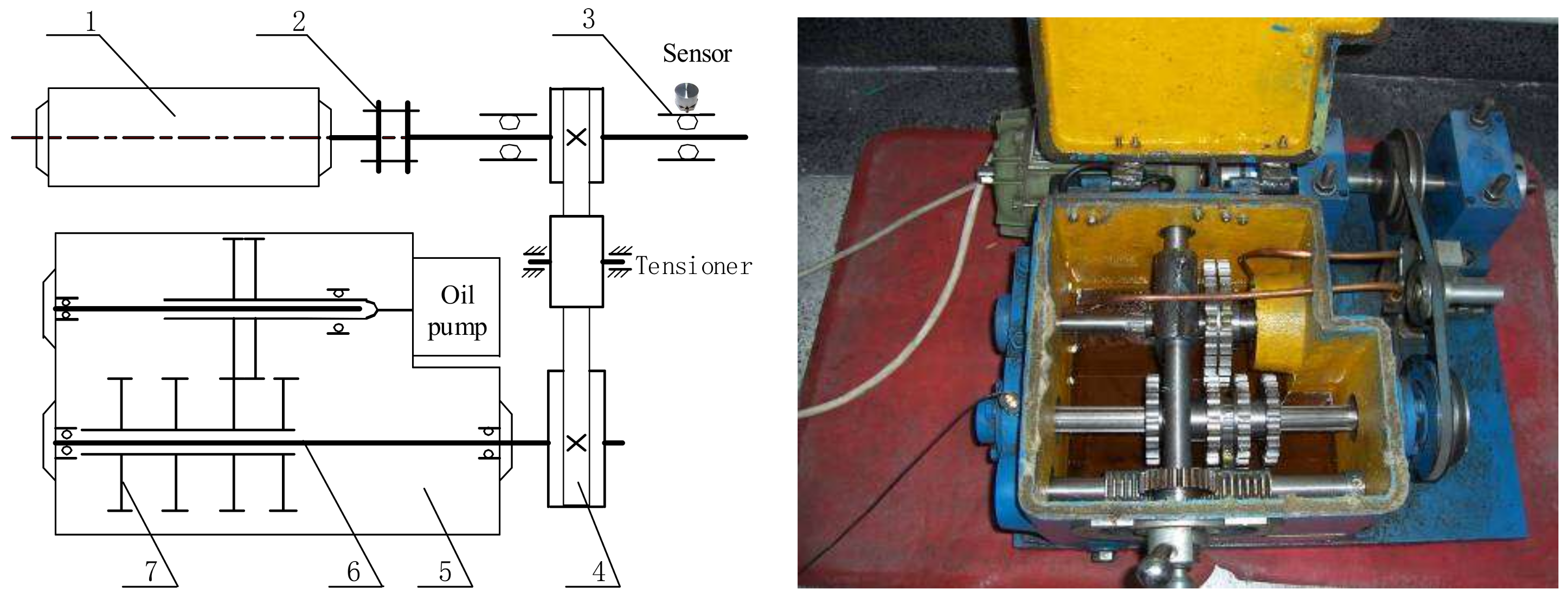
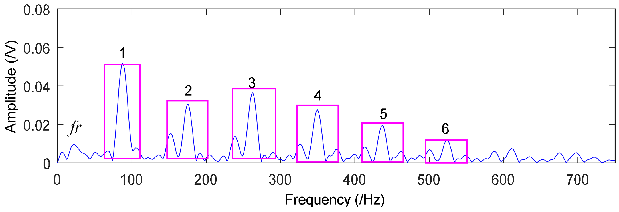
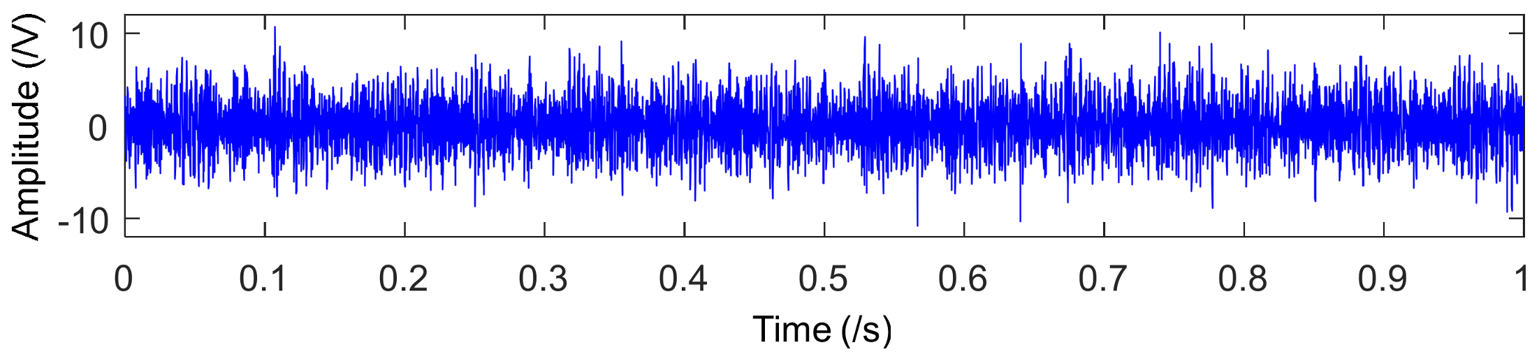
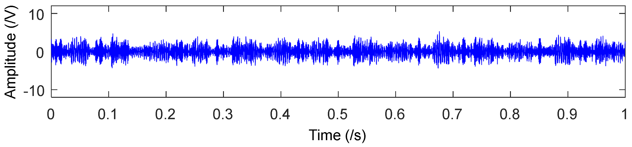
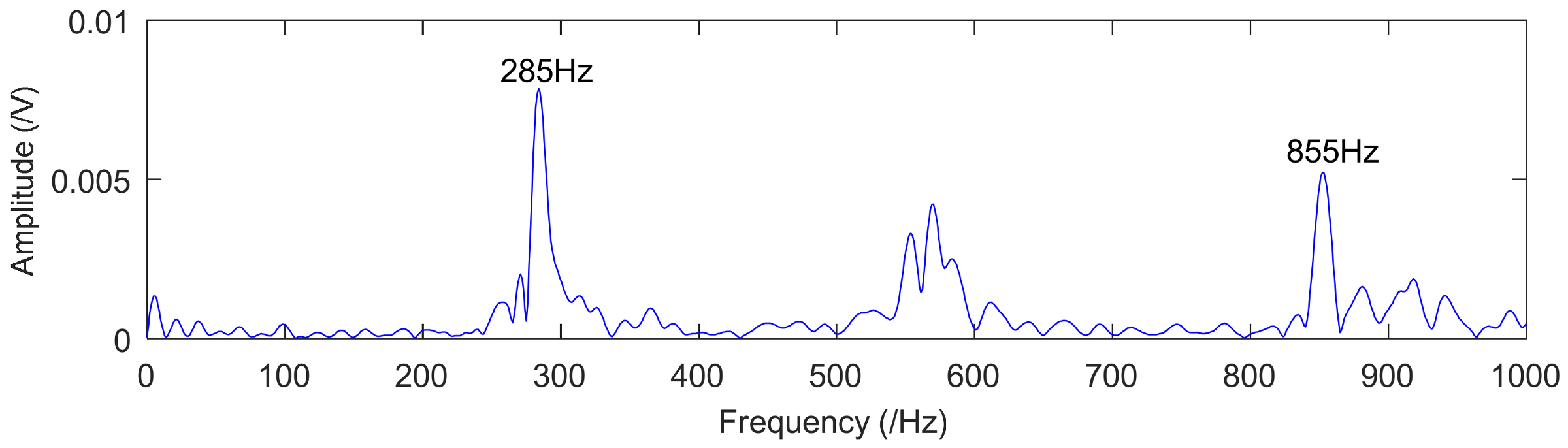
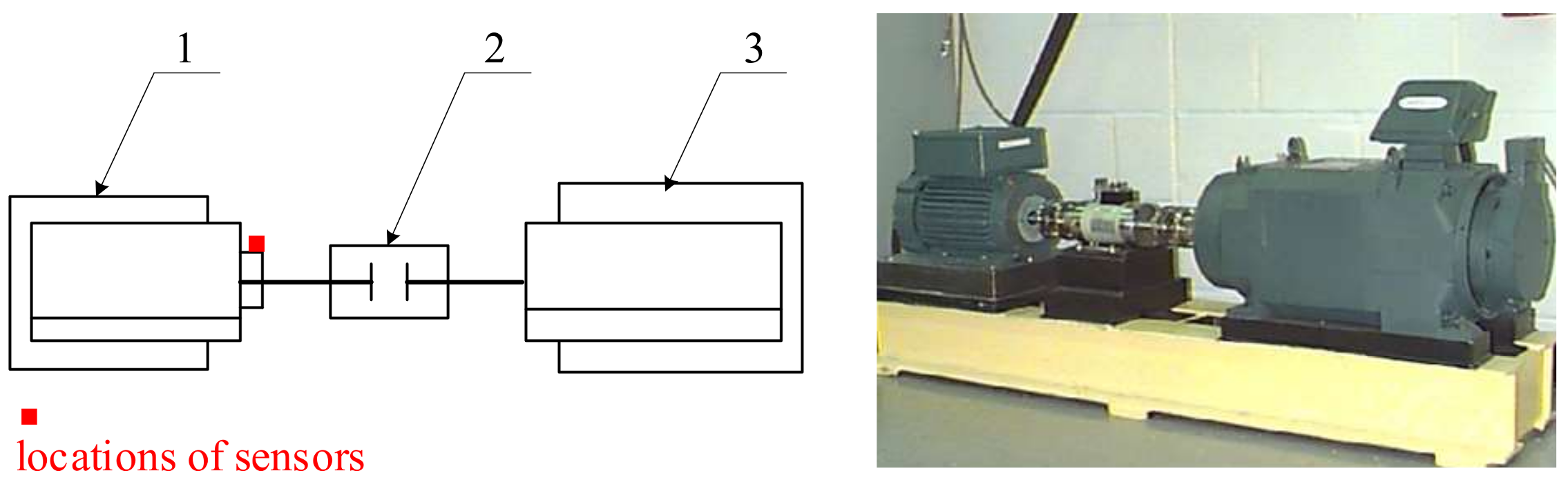
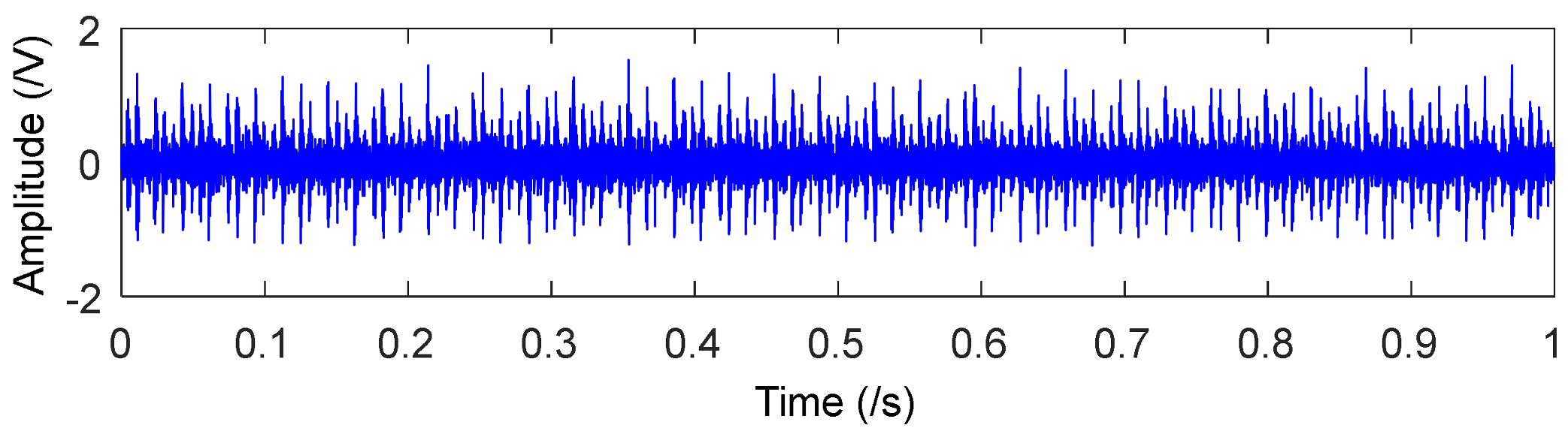
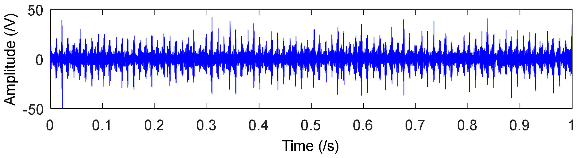
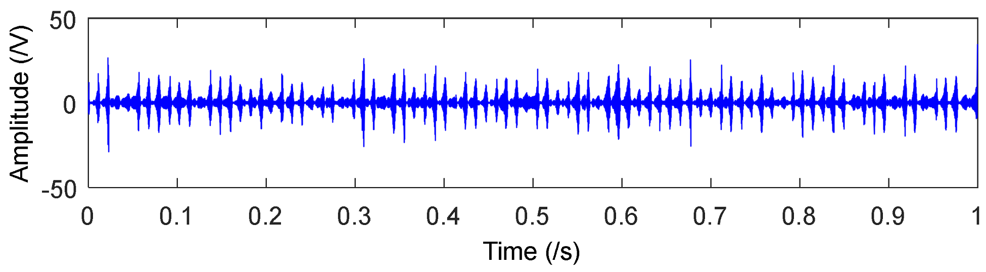
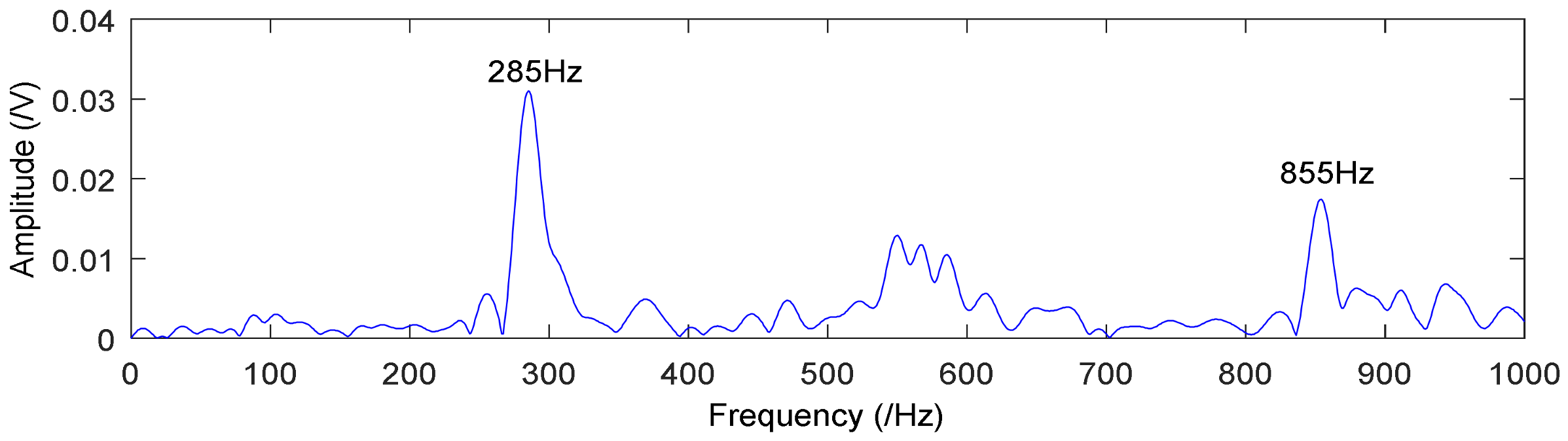
4.2. Application to Drivetrain Diagnostics Simulator
5. Conclusions
Acknowledgments
Author Contributions
Conflicts of Interest
References
- Zhang, S.; Wang, Y.; He, S.; Jiang, Z. Bearing fault diagnosis based on variational mode decomposition and total variation denoising. Meas. Sci. Technol. 2016, 27, 075101. [Google Scholar] [CrossRef]
- Lv, Y.; Yuan, R.; Song, G. Multivariate empirical mode decomposition and its application to fault diagnosis of rolling bearing. Mech. Syst. Sign. Proc. 2016, 81, 219–234. [Google Scholar] [CrossRef]
- Li, K.; Su, L.; Wu, J.; Wang, H.; Chen, P. A Rolling Bearing Fault Diagnosis Method Based on Variational Mode Decomposition and an Improved Kernel Extreme Learning Machine. Appl. Sci. 2017, 7, 1004. [Google Scholar] [CrossRef]
- Fan, Y.S.; Zheng, G.T. Research of high-resolution vibration signal detection technique and application to mechanical fault diagnosis. Mech. Syst. Sign. Proc. 2007, 21, 678–687. [Google Scholar] [CrossRef]
- Glowacz, A.; Glowacz, W.; Glowacz, Z.; Kozik, J. Early fault diagnosis of bearing and stator faults of the single-phase induction motor using acoustic signals. Measurement 2018, 113, 1–9. [Google Scholar] [CrossRef]
- Glowacz, A.; Glowacz, W.; Glowacz, Z. Recognition of armature current of DC generator depending on rotor speed using FFT, MSAF-1 and LDA. Eksploat. Niezawodn. 2015, 17, 64–69. [Google Scholar] [CrossRef]
- Caesarendra, W.; Kosasih, B.; Tieu, A.K.; Moodie, C.A. Application of the largest Lyapunov exponent algorithm for feature extraction in low speed slew bearing condition monitoring. Mech. Syst. Sign. Proc. 2015, 50, 116–138. [Google Scholar] [CrossRef]
- Chibani, A.; Chadli, M.; Peng, S.; Braiek, N.B. Fuzzy fault detection filter design for t-s fuzzy systems in finite frequency domain. IEEE Trans. Fuzzy Syst. 2017, 25, 1051–1061. [Google Scholar] [CrossRef]
- Chadli, M.; Davoodi, M.; Meskin, N. Distributed state estimation, fault detection and isolation filter design for heterogeneous multi-agent linear parameter-varying systems. IET Contr. Theory Appl. 2016, 11, 254–262. [Google Scholar] [CrossRef]
- Mandic, D.P.; ur Rehman, N.; Wu, Z.; Huang, N.E. Empirical mode decomposition-based time-frequency analysis of multivariate signals: The power of adaptive data analysis. IEEE Sign. Proc. Mag. 2013, 30, 74–86. [Google Scholar] [CrossRef]
- Aguiar-Conraria, L.; Soares, M.J. The continuous wavelet transform: Moving beyond uni-and bivariate analysis. J. Econ. Surv. 2014, 28, 344–375. [Google Scholar] [CrossRef]
- Gilles, J. Empirical wavelet transform. IEEE Trans. Sign. Proc. 2013, 61, 3999–4010. [Google Scholar] [CrossRef]
- Zhou, B.; Liu, Z. Method of multi-resolution and effective singular value decomposition in under-determined blind source separation and its application to the fault diagnosis of roller bearing. In Proceedings of the 2015 11th International Conference on Computational Intelligence and Security (CIS), Shenzhen, China, 19–20 December 2015; pp. 462–465. [Google Scholar]
- Cawley, R.; Hsu, G.H. Local-geometric-projection method for noise reduction in chaotic maps and flows. Phys. Rev. A 1992, 46, 3057–3082. [Google Scholar] [CrossRef] [PubMed]
- Sauer, T. A noise reduction method for signals from nonlinear systems. Phys. D 1992, 58, 193–201. [Google Scholar] [CrossRef]
- Kantz, H.; Schreiber, T. Nonlinear Time Series Analysis; Cambridge University Press: Cambridge, UK, 2003. [Google Scholar]
- Cao, L. Practical method for determining the minimum embedding dimension of a scalar time series. Phys. D Nonlinear Phenom. 1997, 110, 43–50. [Google Scholar] [CrossRef]
- Wang, G.F.; Li, Y.B.; Luo, Z.G. Fault classification of rolling bearing based on reconstructed phase space and Gaussian mixture model. J. Sound Vib. 2009, 323, 1077–1089. [Google Scholar] [CrossRef]
- Vautard, R.; Yiou, P.; Ghil, M. Singular-spectrum analysis: A toolkit for short, noisy chaotic signals. Phys. D Nonlinear Phenom. 1992, 58, 95–126. [Google Scholar] [CrossRef]
- Lv, Y.; He, B.; Yi, C.; Dang, Z. 2366. A novel scheme on multi-channel mechanical fault signal diagnosis based on augmented quaternion singular spectrum analysis. J. Vibroeng. 2017, 19, 955–966. [Google Scholar]
- Michael, T.J.; Richard, J.P. Generalized phase space projection for nonlinear noise reduction. Phys. D 2005, 201, 306–317. [Google Scholar]
- Jevtić, N.; Stine, P.; Schweitzer, J.S. Nonlinear time series analysis of Kepler Space Telescope data: Mutually beneficial progress. Astron. Nachr. 2012, 333, 983–986. [Google Scholar] [CrossRef]
- Kotas, M. Projective filtering of time warped ECG beats. Comp. Biol. Med. 2008, 38, 127–137. [Google Scholar] [CrossRef] [PubMed]
- Grassberger, P.; Schreiber, T.; Schaffrath, C. Nonlinear time sequence analysis. Int. J. Bifurc. Chaos 1991, 1, 521–547. [Google Scholar] [CrossRef]
- Grassberger, P.; Hegger, R.; Kantz, H.; Schaffrath, C.; Schreiber, T. On noise reduction methods for chaotic data. Chaos: An Interdisciplinary. J. Nonlinear Sci. 1993, 3, 127–141. [Google Scholar]
- Chelidze, D. Smooth local subspace projection for nonlinear noise reduction. Chaos Interdiscip. J. Nonlinear Sci. 2014, 24, 013121. [Google Scholar] [CrossRef] [PubMed]
- Moore, J.M.; Small, M.; Karrech, A. Improvements to local projective noise reduction through higher order and multiscale refinements. Chaos Interdiscip. J. Nonlinear Sci. 2015, 25, 063114. [Google Scholar] [CrossRef] [PubMed]
- Tugnait, J.K.; Luo, W. On channel estimation using superimposed training and first-order statistics. In Proceedings of the 2003 IEEE International Conference on Acoustics, Speech, and Signal Processing, Hong Kong, China, 6–10 April 2003; Volume 4. [Google Scholar]
- Tong, L.; Xu, G.; Kailath, T. Blind Identification and equalisation based on second-order statistics: A time domain approach. IEEE Trans. Inf. Theory 1994, 40, 340–349. [Google Scholar] [CrossRef]
- Rosa, J.; Lloret, I.; Puntonet, C.G.; Piotrkowski, R.; Moreno, A. Higher-order spectra measurement techniques of termite emissions. A characterization framework. Measurement 2008, 41, 105–118. [Google Scholar] [CrossRef]
- Chua, K.C.; Chandran, V.; Acharya, U.R.; Lim, C.M. Application of higher order statistics/spectra in biomedical signals—A review. Med. Eng. Phys. 2010, 32, 679–689. [Google Scholar] [CrossRef] [PubMed] [Green Version]
- Zheng, K.; Li, T.; Zhang, B.; Zhang, Y.; Luo, J.; Zhou, X. Incipient Fault Feature Extraction of Rolling Bearings Using Autocorrelation Function Impulse Harmonic to Noise Ratio Index Based SVD and Teager Energy Operator. Appl. Sci. 2017, 7, 1117. [Google Scholar] [CrossRef]
- Jiang, Z.; Hu, M.; Feng, K.; He, Y. Weak fault feature extraction scheme for intershaft bearings based on linear prediction and order tracking in the rotation speed difference domain. Appl. Sci. 2017, 7, 937. [Google Scholar] [CrossRef]
- Loparo, K.A. Bearings Vibration Data Set, Case Western Reserve University. Available online: http://csegroups.case.edu/bearingdatacenter/home (accessed on 30 October 2017).
- Mendel, J.M. Tutorial on higher-order statistics (spectra) in signal processing and system theory: Theoretical results and some applications. Proc. IEEE 1991, 79, 278–305. [Google Scholar] [CrossRef]
- Nikias, C.L.; Mendel, J.M. Signal processing with higher-order spectra. IEEE Sign. Proc. Mag. 1993, 10, 10–37. [Google Scholar] [CrossRef]


| Methods | MSE | CC |
|---|---|---|
| Standard local projection | 1.2392 | 0.9826 |
| Multiscale local projection | 0.7939 | 0.9949 |
| Rolling Element Bearing Parameters of 6205-2RS JEM SKF | |||||
|---|---|---|---|---|---|
| Inside Diameter d1 (mm) | Outside Diameter d2 (mm) | Ball Number n | Ball Diameter dr (mm) | Contact Angle | Pitch Diameter Dw (mm) |
| 25 | 52 | 9 | 7.9 | 0 | 46.4 |
| Rotation Frequency fr (Hz) | Inner fi (Hz) | Outside fo (Hz) | Ball fb (Hz) | Cage fc (Hz) |
|---|---|---|---|---|
| 29.53 | 159.92 | 105.87 | 139.20 | 11.69 |
| Rotating Speed r (min) | Rotating Frequency fr (Hz) | Sampling Frequency (Hz) | Sampling Points | Outer Fault Frequency fo (Hz) |
|---|---|---|---|---|
| 1450 | 24.17 | 16,384 | 16,380 | 87.01 |
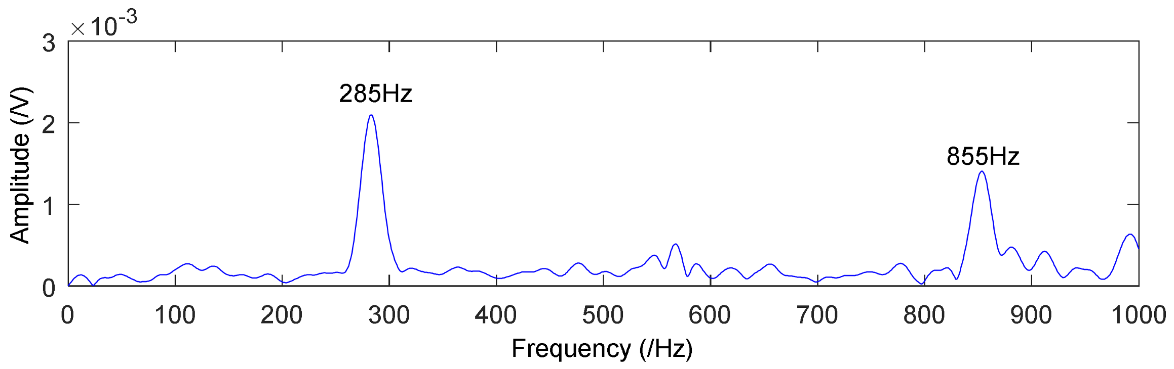
| Rotating Speed r (min) | Rotating Frequency fr (Hz) | Sampling Frequency (Hz) | Sampling Points | Fault Frequency f (Hz) |
|---|---|---|---|---|
| 855 | 14.25 | 8192 | 8192 | 285 |
© 2018 by the authors. Licensee MDPI, Basel, Switzerland. This article is an open access article distributed under the terms and conditions of the Creative Commons Attribution (CC BY) license (http://creativecommons.org/licenses/by/4.0/).
Share and Cite
Lv, Y.; Yuan, R.; Shi, W. Fault Diagnosis of Rotating Machinery Based on the Multiscale Local Projection Method and Diagonal Slice Spectrum. Appl. Sci. 2018, 8, 619. https://doi.org/10.3390/app8040619
Lv Y, Yuan R, Shi W. Fault Diagnosis of Rotating Machinery Based on the Multiscale Local Projection Method and Diagonal Slice Spectrum. Applied Sciences. 2018; 8(4):619. https://doi.org/10.3390/app8040619
Chicago/Turabian StyleLv, Yong, Rui Yuan, and Wei Shi. 2018. "Fault Diagnosis of Rotating Machinery Based on the Multiscale Local Projection Method and Diagonal Slice Spectrum" Applied Sciences 8, no. 4: 619. https://doi.org/10.3390/app8040619