Article

Energy Management Strategy for Rural Communities’ DC Micro Grid Power System Structure with Maximum Penetration of Renewable Energy Sources

by
Maheswaran Gunasekaran
1,
Hidayathullah Mohamed Ismail
1,
Bharatiraja Chokkalingam
1,
Lucian Mihet-Popa
2,* and
Sanjeevikumar Padmanaban
3
1
Department of Electrical and Electronics Engineering, SRM University, Chennai 603 203, India
2
Faculty of Engineering, Østfold University College, Kobberslagerstredet 5, 1671 Kråkeroy-Fredrikstad, Norway
3
Department of Energy Technology, Aalborg University, Esbjerg 6700, Denmark
*
Author to whom correspondence should be addressed.
Appl. Sci. 2018, 8(4), 585; https://doi.org/10.3390/app8040585
Submission received: 19 January 2018 / Revised: 5 March 2018 / Accepted: 12 March 2018 / Published: 8 April 2018
(This article belongs to the Special Issue DC & Hybrid Micro-Grids)

Abstract

:
The AC and DC power system structures need to be modernized to meet consumer demands. DC microgrids are suitably admired due to their high efficiency, consistency, reliability, and load sharing performance, when interconnected to DC renewable and storage sources. The main control objective for any DC microgrid is providing proper load–power balancing based on the Distributed Generator (DG) sources. Due to the intermittent nature of renewable energy sources, batteries play an important role in load–power balancing in a DC microgrid. The existing energy management strategy may be able to meet the load demand. However, that technique is not suitable forrural communities’ power system structure. This research offers an energy management strategy (EMS) for a DC microgrid to supply power to rural communities with solar, wind, fuel cell, and batteries as input sources. The proposed EMS performs the load–power balancing between each source (renewable and storage) in a DC microgrid for dynamic load variation. Here, the EMS handles two battery sources (one is used to deliver power to the priority load, and the other is utilized in the common DC bus) to meet the required demand. The proposed EMS is capable of handling load–power balancing using renewable energy sources with less consumption of non- conventional energy sources (such as a diesel generator). The performance of the system is analyzed based on different operating conditions of the input sources. The MATLAB/Simulink simulation model for the proposed DC microgrid with their EMS control system is developed and investigated, and their results are tabulated under different input and load conditions. The proposed EMS is verified through a laboratory real-time DC microgrid experimental setup, and the results are discussed.

1. Introduction

Today, the world population is drastically increasing, hence the consumption of electrical energy is increasing accordingly. Since 75% of people are residents of the metropolitan areas and 25% of people live in remote villages, the majority of the power supplied to these areas is generated using fossil fuels rather than the renewable energy sources. Hence, the usage of fossil fuelswill result in 60% environmental depletion. Today, many countries have started to generate power through non-conventional energy sources compared to conventional energy sources. Considerable investments in distributed energy resources have taken place even during and after the financial crisis affecting the world economy from 2008 to 2012. As per an international energy agency report on world energy investment in 2017, China, the United States, Europe, India, Russia, and South Africa have invested a considerable amount to harvest renewable energies in comparison to other countries [1]. According to the international energy investment report [2], many countries have started investing much in solar and wind rather than other renewable energy sources.
The best solution to overcome environmental depletion is by harvesting a renewable energy–sourced microgrid. Most of the non-conventional energy sources are synchronized with the utility or load through power converter interfaces, which constitutes a microgrid. Microgrids are sub-categorized into three types: AC, DC, and hybrid [3]. AC microgrids have the benefit of using power from the utility.However, an AC microgrid needs a relatively complex controller for synchronizing the system and importing and exporting power while maintaining system stability. The DC microgrid has certain advantages with many features. On the generation side, some of the renewable energy sources, generating power in a DC microgrid include fuel cells and photovoltaic and storage systems, whereas on the load side, modern electronic loads like computers, telephone base stations, vehicle charging stations, and telecommunication applications require DC power. Both the AC and DC loads will be fulfilled by a hybrid microgrid. The main advantage of a microgrid is having a less transmission loss, electrification of remote villages, improving power system stability by supporting reactive power balance in the utility grid, and high reliability with energy storage devices to sustain power balance among the generation and demand. The total energy conversion loss of AC to DC to supply DC loads is approximately 10–25% [4,5]. To resolve this issue, the DC microgrid feeds the load directly, which will reduce the conversion loss [6,7]. For remote village communities, the DC microgrid is the most preferred power supplying utility because the main utility grid may not electrify these village communities because of transmission issues. Therefore, the residential, lighting and commercial loads will be met by the DC microgrid with the help of a battery [8,9,10,11]. The battery energy storage system will be important in the DC microgrid because the batteries are charged during non-peak load condition and discharged during peak load condition with some fluctuations in the power generated by the renewable energy sources [11,12,13,14]. There are several research areas on the subject of the microgrid, of which the demand side management (DSM) is the main focus area. It will adjust the demand with respect to the consumers’ requirements with respect to time (kW/h). Therefore, the utility can reduce the peak load and reduce congestion in the system.
This system will decrease the difference between the peak load and total generation at peak time periods [15,16,17]. The transition from a minimum load to maximum load approachingthe compress load curve is a great advantage of demand-side management in microgrid applications. The energy storage has different ramp rates, which are used to reduce the deviation in the voltage and improve stability [15]. Biomass is one of the non-conventional energy sources that generate power in small capacity and that is also integrated into the DC microgrid to supply power to remote communities [16]. However, by integrating the various sources into the grid, protection has to be considered for the DC microgrid, which is discussed in [17,18]. The depth penetration of renewable energy sources into the microgrid and EMS when considering the intermittent of photovoltaic systems is proposed in [19,20]. The main control function of EMS in any DC microgrid structure is to handle the load–power balancing. It should be reliable and cost-effective based on the power obtained from the distributed generation [18,19,20]. A conventional EMS has some ability to meet the above-mentioned problems for the DC microgrid structure. A rural community microgrid design and a review of the various architectures in some countries are discussed in [21,22]. Power quality is one of the issues in hybrid and AC microgrids [21,22,23,24,25,26]. This research work will focus on the EMS for a DC microgrid to supply remote village communities. The proposed EMS overcomes the drawbacks of the conventional system by load–power balancing between each source (renewable and storage) in a DC microgrid for dynamic load variation and reduces the consumption of non-conventional energy sources (such as a diesel generator). The general concept of the microgrid, the load profile of the village communities, and the functional block diagram of the proposed DC microgrid are discussed in Section 2. In Section 3, the mathematical modeling of different renewable energy sources is discussed. In Section 4, the proposed EMS is discussed. The simulation studies and experimental results are discussed in Section 5 and Section 6. Finally, the DC microgrid system is concluded in Section 7.

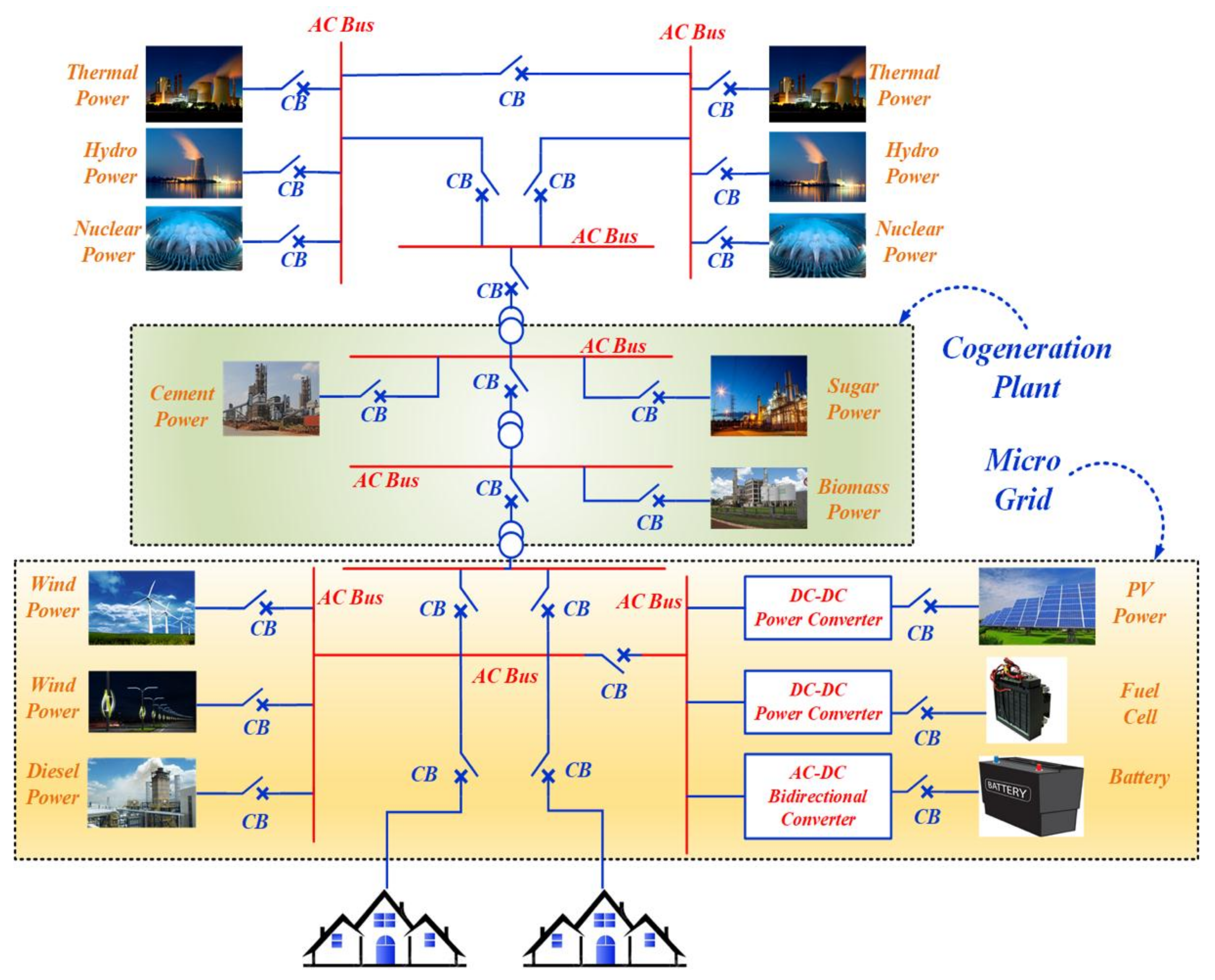
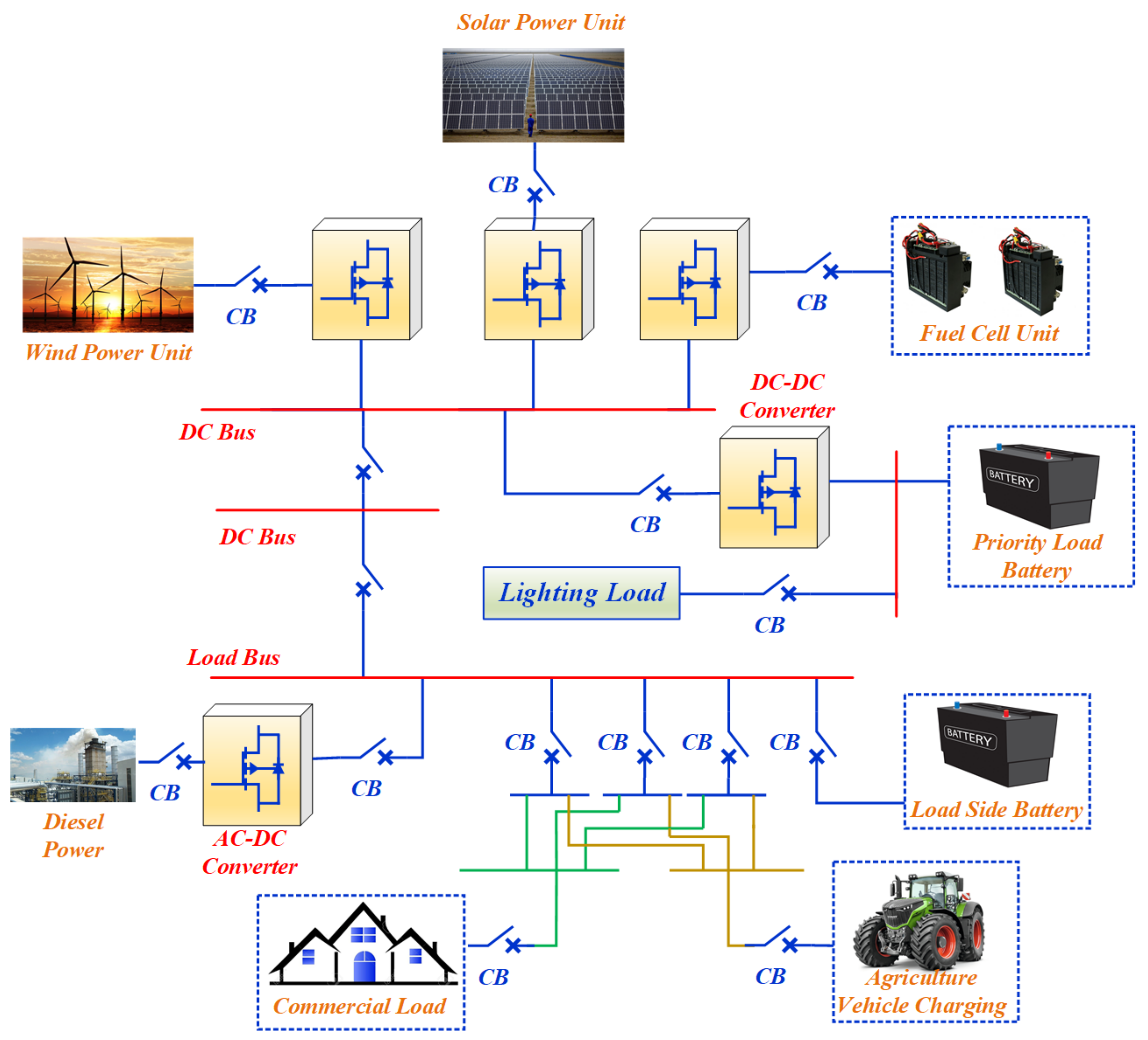
2. Power System Network

The power system network is comprised of generation, transmission, and distribution. In generation, all the power generation plants, like thermal, hydro, nuclear etc., are connected in parallel. The generated power is stepped up and transmitted to reduce transmission loss. Finally, in the distribution stage, the power is supplied to different types of consumers with respect to their requirements. Figure 1 shows the schematic structure of the power system network. There are two thermal units, two hydro, and two nuclear power generation units that are connected in parallel, which will be connected to the transmission network. In the second stage of the transmission network, the co-generation plants like sugar plants and cement plants are connected to the distribution bus, and finally, in the distribution network, the voltage is stepped down, and it will supply power to different consumers like industrial, commercial, and domestic consumers. The power fluctuation severely affects consumers in the distribution stage, which is limited to some extent through the use of the microgrid, which is supplied through renewable energy sources like wind, PV, fuel cells, and diesel power. The main advantage of the microgrid is that it is able to instantaneously meet any increase in load that cannot be reciprocated by thermal, hydro, and nuclear generating units. The liability of the system will improve, and the microgrid is a better solution for supplying power to a remote village community.

Proposed DC Microgrid Architecture for Rural Communities

The proposed DC microgrid architecture is for remote villages. In a village, the various loads such as commercial loads, agricultural vehicle loads, and priority load (street lighting) are considered. The power generation capacity of each sourceis 5 kW, as shown in Figure 2. The power generated in the fuel cell and PV is DC, but for wind it is AC, so the AC is converted into DC by means of a converter.
To reduce voltage variation, a converter is used in all DG sources. The power produced from non-conventional energy sources areinconsistent to supply load continuously due to its intermittent. Therefore, batteries are utilized to ensure power supply to consumers without any interruption. Here, two batteries are used. One is interfaced to the load side, and the other is on the DC bus. The DC bus battery is only used for the priority load, and the load side battery is used for the commercial and agricultural vehicle loads. The diesel generator is also connected to the DC distribution network to deliver the load when available power in the DC microgrid is not sufficient. AC power generated by the diesel generator is converted to DC power by a converter.

3. Mathematical Modeling of ProposedDC Architecture

The proposed DC microgrid consists of four different sources (PV, wind, fuel cell, and battery). The PV power mainly depends upon solar irradiance and the ambient temperature. Wind power depends on wind velocity. PMSG is used to generate electrical power from the turbine. Wind power is interconnected to the DC microgrid by the AC/DC converter. Fuel cell power depends upon parameters such as distribution, flow rate, partial pressure of fuel cell gases, and the required number of stack cells. Mathematical modeling of each source is briefly discussed in this section.

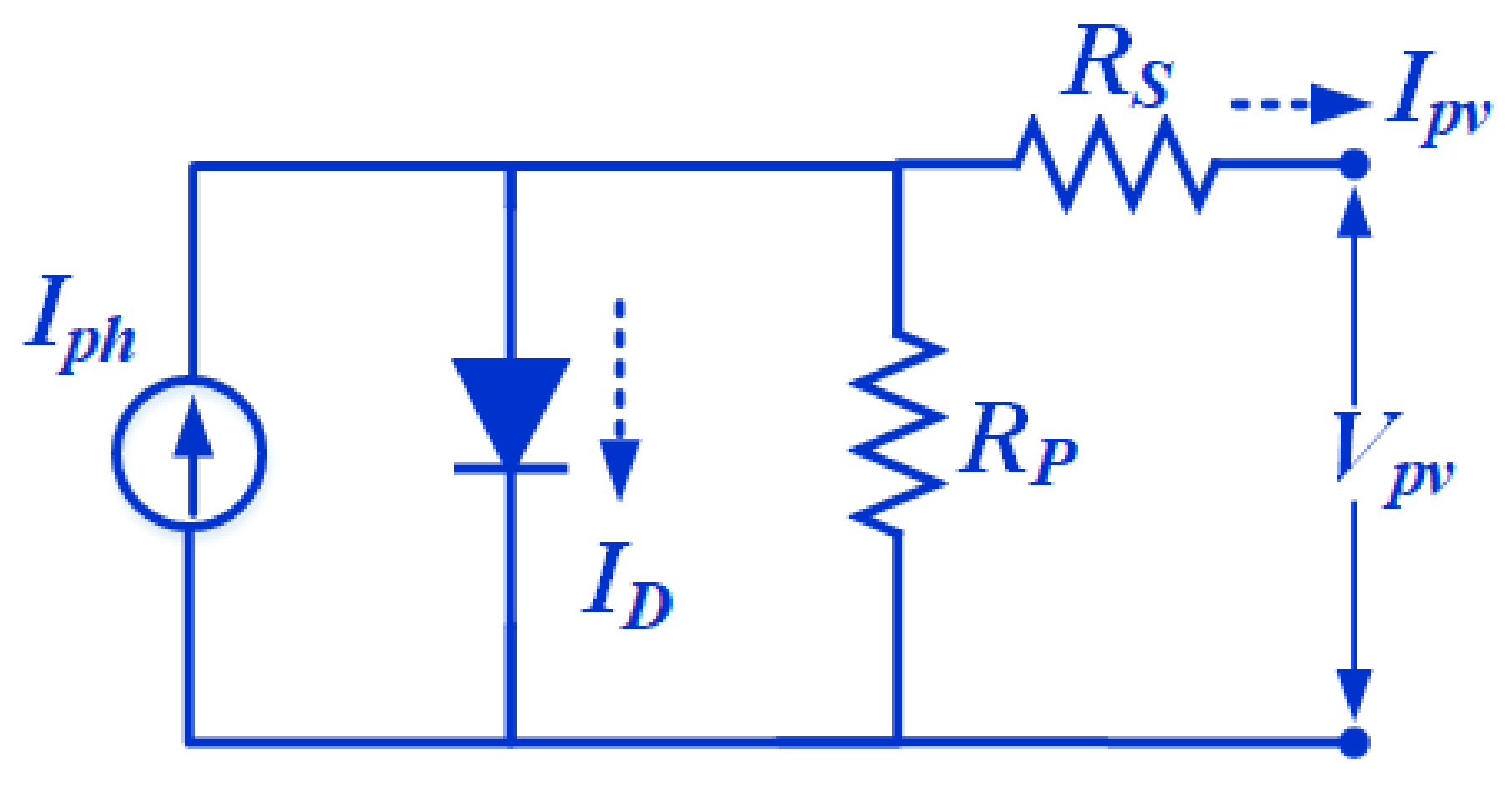
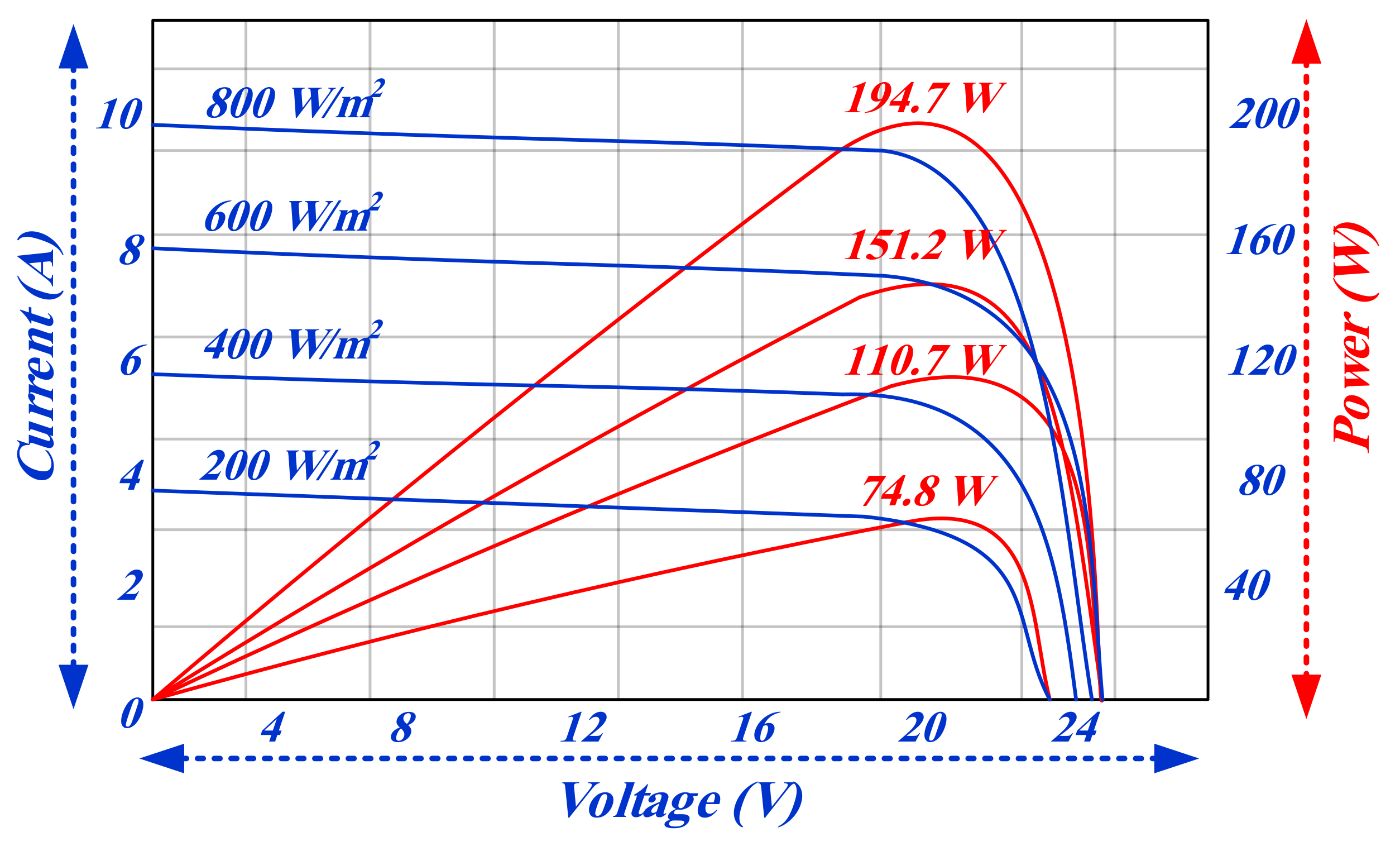
3.1. Mathematical Modeling of Solar Power

The output power of the PV module is obtained by solar irradiance and with respect to PV module area. The output of the PV model is determined by [23]
P s o l a r = η g i r A ,
where, η g = generation efficiency, i r = solar irradiation (W/m2) and A = area (m2), and the PV efficiency is determined by Equation (2).
η c e = η r e f η c e [ 1     β ( T c e l l     T c e l l r e f ) ] ,
where, η c e = power conditioning efficiency, β = Temperature co-efficient C ((0.004–0.006)/C), η r e f = reference module efficiency, T c e l l r e f = reference cell temperature, and the temperature ( T C ) is determined by Equation (3).
T c = T a + [ N O C T 20 800 ] G t ,
where, T a = temperature in C, NOCT = nominal operating cell temperature in C, G t = solar irradiation in tilted module (W/m2).
Total radiation in the solar cell considering normal and partial solar radiation is obtained by
T I = I D R D + ( I b + I d ) R r .

System Modeling

The PV or solar cell operation is similar to the operation of PN junction diode, which converts light energy into electricity through the photovoltaic effect [24]. The PV module is grouped based on the series and parallel connection of multiple PV cell [24,25]. The single PV cell is configured into a single diode representation as in Figure 3. In this model, solar irradiance is represented by a current source, and the other circuit parameters are diode current Id, output current I, series resistance Rs, parallel resistance Rp, and output voltage V. The output current is calculated by
I = N P [ I p h I r s ( exp q ( V + I R s ) A K T N s 1 ) ] ,
I R S = I r r [ 1 T K 1 T ] ,
where, NP and NS = number of cell connected in parallel and series, the K = Boltzmen constant, A = diode ideality factor, IRS = reverse saturation current of cell at T, Tr = referred cell temperature, and Irr = reverse saturation current at Tr
I p h = [ I s c r + K i ( T     T r ) S 100 ] ,
where, Iscr = short circuit current at a reference temperature of the cell, Ki = co-efficient of the short circuit temperature, S = solar irradiation in (W/m2). In this model, the shunt resistance in parallel to the ideal shunt diode and the I-V characteristics are determined by the equation as follows:
I = I p h I D ,
I = I p h     I o [ exp q ( V + I R s ) A K T 1 ] V + R s I R s h ,
where, Iph = Irradiance current (A), ID = diode current (A), Io = Inverse saturation current (A), RS = series resistance (Ω), Rsh = shunt resistance (Ω), I = cell current (A), V = cell voltage, and the output current of the PV cell using single diode model is expressed as
I = I P V     I D 1     V + I R s R s h .
The open circuit voltage and maximum power of the PV module is obtained by the simplified PV system modeling proposed by [26]. The voltage and power with the values of series resistance (RS) is calculated by fill factor [27,28,29].
F F = F F o [ 1     R s V O C I S C ] F F o = V O C ln ( V O C + 0.72 ) 1 + V V O C }
P max = F F ×   V O C ×   I O C P max = V O C ln ( V O C + 0.72 ) 1 + V O C ×   ( 1 I S C ×   R S V O C ) ×   V O C O 1 + β ln G O G ×   ( T O T ) δ ×   I S O ( G G O ) α }
where, FF = fill factor of the ideal PV module without resistive effects and VOC = normalized value of the open circuit voltage to thermal voltage.
The power conversion in the PV system is obtained through the PV modules. The performance capability of the PV depends on the temperature and its characteristic curve (power & V, I curve) at standard test condition, which is shown in Figure 4. A single PV cell of any rating will not be able to generate the required power levels. Hence, several PV cells are interconnected through a series and parallel combinations that scale up to generate the required PV power. The voltage and current are obtained by scaling up of PV modules, which is expressed as
I A = N p I M V A = N S ×   V M P A = F F ×   V A ×   I A }
where, IA and VA = PV array voltage and current, IM and VM = PV module voltage and current, and PA and PM = PV array power and module power.

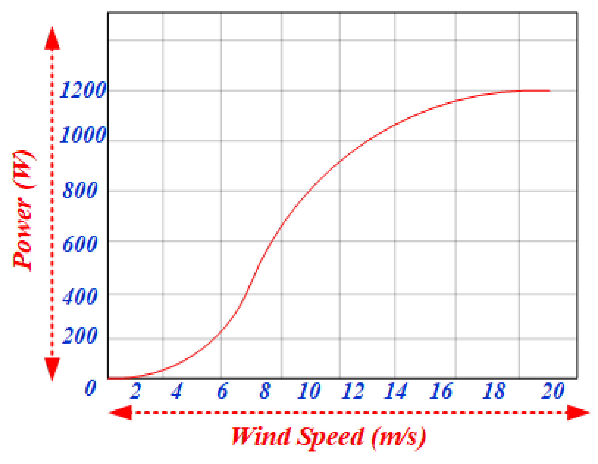
3.2. Mathematical Modeling of Wind Power

The wind model consists of variation of wind velocity with gust and wind speed [30,31,32,33,34,35,36].
W V = V w +   V g + V w r ,
where, Vw = Base wind velocity, Vg = Gust wind velocity, and Vwr = ramp wind component.
The gust speed is calculated by
V w g = { 0   t < T 1 C 2 { 1 cos π [ t T 1 T 2 T 1 ] T 1 t T 2 } 0   t T 2 }
V W = { 0   s < T 3 C 3 { [ s T 3 T 4 T 3 ] T 3 s T 4 } 0   s T 4 } ,
where, C2 = maximum value of the gust component, C3 = maximum wind speed caused by the ramp, and T3 and T4 are the cut-in and cut-out times of the ramp, respectively.
Wind power is calculated by
P W = d W w d t
Energy drawn by the wind turbine is
W w = V a × 1 2 ρ ( V 1 2 V 3 2 ) P W = d V a 1 2 ρ ( V 1 2 V 3 2 ) d t }
where, W w = energy drawn by wind turbine and ρ = Air density.
According to Betz, the maximum wind turbine power output is
P M = 16 27 A R 3 2 V 3
Equation (19) is obtained by substituting the value for V1, and V3.
V 2 = 2 3 V 1 V 3 = 1 3 V 1
The wind turbine model represents the output power captured by the turbine [33,34,35,36]. Figure 5 shows the characteristic curve for wind speed vs. power. The power in the wind (Pw) in an area is obtained by
P W = 1 2 ρ A W V 3
P M = P W C p
C P = 1 2 [ δ     0.22 β 2     5.6 ) e 0.17 δ
β = Pitch angle of the blade in degrees, δ = the tip speed ratio of the turbine, and C p = Power coefficient.
Wind generated power is expressed as:
p G = V G I G

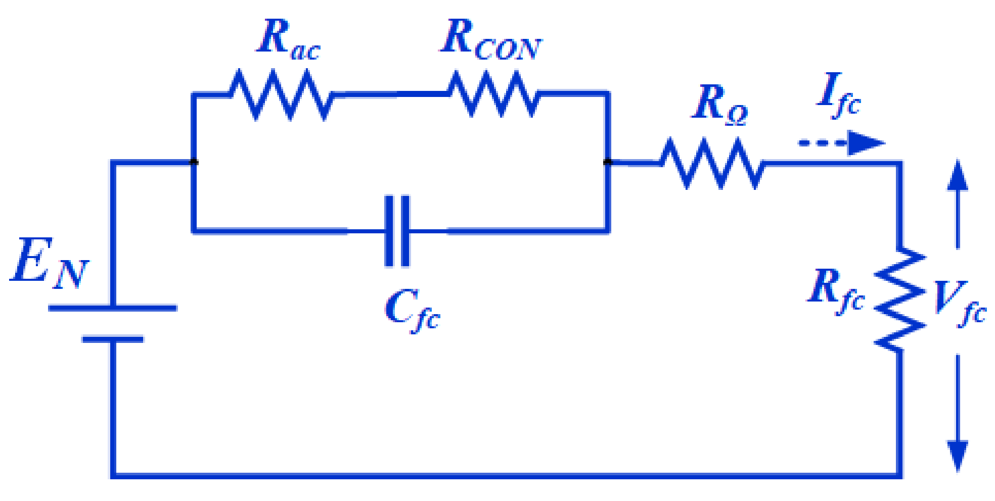
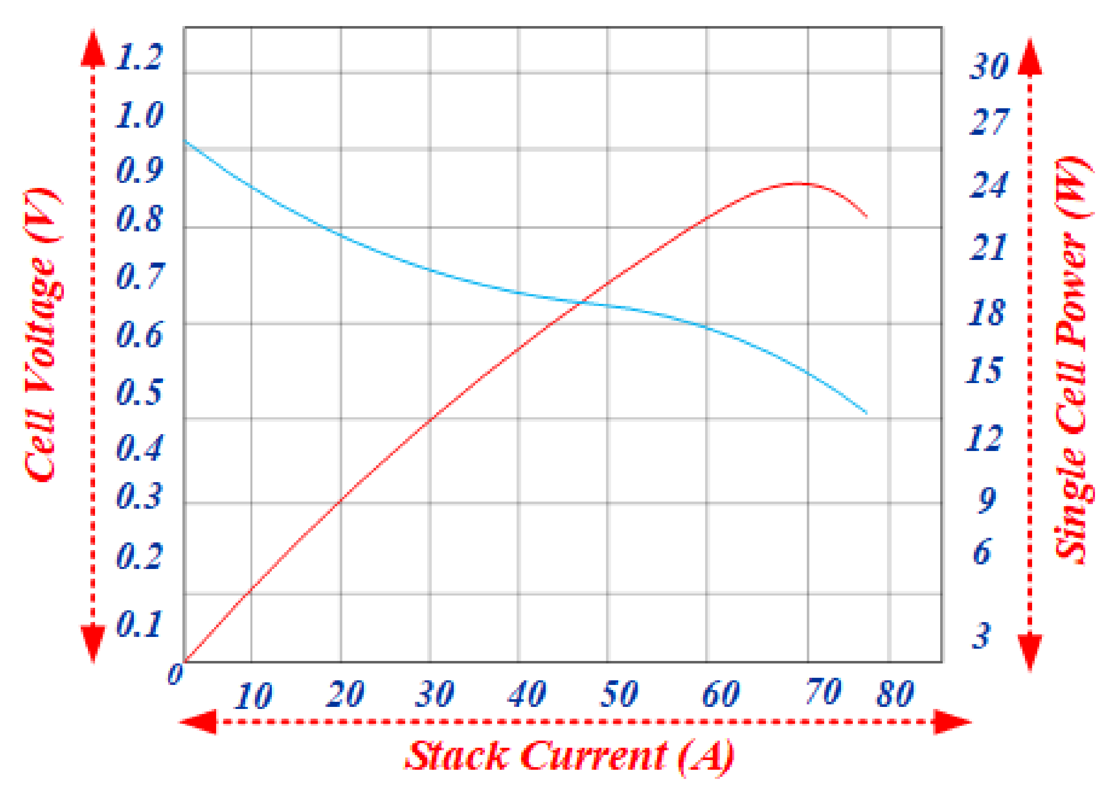
3.3. Mathematical Modeling of Fuel Cell Power

A different assumption [36] is made, which is described below:
  • Idealized modeling;
  • Uniform circulated gases;
  • Constant pressure in the flow channel;
  • Cell parameters are represented together to form stack parameters;
  • The output voltage of the single fuel cell can be represented as
    P H 2 = 1 t H 2 [ P H 2 + 1 K H 2 ( q t h i n 2 K r i F C ) ] P O 2 = 1 t O 2 [ P O 2 + 1 K O 2 ( q t h i n 2 K V i F C ) ] P H 2 O = 1 t H 2 O [ P H 2 O + 1 K H 2 O K r i F C ] }
Here, KH2 = valve meter constant for hydrogen and KO2 = valve meter constant for oxygen (2.52 × 10⁻³ kmol/s atm). Kr = constant defined by the rate of reactant hydrogen and fuel cell current. The reactant utilization factor U is defined as follows:
U F = q H 2 i n     q H 2 o u t q H 2 i n
V a c t = [ E 1 + E 2 T + E 3 T l n ( c o 2 ) + E 4 l n ( i F C ) ] c o 2 = p o 2 5.08 × 10 6 e ( 498 T )
where, E1, E2, E3, E4 is the cell parameter coefficients, CO2 = concentration of oxygen. Figure 6 represents the equivalent circuit of the fuel cell. It consists of cell voltage, actual resistance, concentration resistance, and ohmic resistance [37,38].
V o h m = i F C ( R m + R o h m )
R m = ρ m l A
where, ρ m = specific resistivity of the membrane for electron flow (Ω cm). A = active cell area (cm2) and l = thickness of the membrane.
The concentration loss is due to the reactive excess concentration near the catalyst surface.
V C o n = R c o n T 2 F ln ( 1 j j max )
The fuel cell current can be determined as
i = i o A ( e α n f P f C V a c t e ( 1 α ) n F V a c R T F C )
Io = exchange current density (A/m2), A = catalyst layer surface (m2), and i = fuel cell current. The Figure 7 shows the single fuel cell characteristics for stack current vs. cell voltage and power. The power of the fuel cell can be obtained from
P f u e l = V o u t i C .

3.4. Mathematical Modeling of the Battery

The mathematical models of the battery focus mainly on V, I parameters. The current is determined by a change in the terminal voltage of the battery [36]. The transfer of electrons from one electrode to another leads to the generation of current. The open circuit voltage at the battery is determined from the potential difference between the positive and negative electrodes [37,38,39,40]. The charging/discharging of battery is expressed as
V d i s c h a r g e = E o V o p + V o p I R p o l
V c h a r g e = E o + V o p + + V o p + I R p o l
V b a t t e r y = E o     K [ Q Q     i t ] i     R o i
V b a t t e r y = E o     ( K S o c ) i     R o i
V d i s c h a r g e = E o     K d r Q Q     i t i 1     R o i     K d v Q Q     i t i t + e ( t )
V c h a r g e = E o     K c r Q i t + λ Q i 1     R o i     K c v Q Q     i t i t + e ( t )
e ( t )   =   B i [ ( e ( t )   +   A u ( t ) ]
V d i c h a r g e = E o     K d r 1 S o c i     R o i     K V ( 1 S o c   1 ) + e ( t )
Equation (35) can be rewritten using state of charge (SoC) due to the polarization ohmic voltage. Equations (37) and (38) are modified by the shepherd relation model. Eo = open circuit voltage of a battery (V), K = polarization coefficient (Ω), Q = battery capacity (A/h), and R = internal resistance. Some of the limitations associated with Equations (37) and (38) are (i) ageing of battery and self-discharge, (ii) the battery capacity does not depend upon the amplitude of the current, and (iii) the temperature coefficient is not considered [35]. These limitations can be overcome by considering the factors affecting the lifetime of the battery. The SoC condition is analyzed at every instant of time and is calculated with threshold capacity using
S o c = S o c i n 0 t ( i max ( i g , i d ) ) d τ Q .
The net power of the DC microgrid architecture is calculated by the summing of all the power of the energy sources.
P n e t = P P V + P W i n d + P f u e l c e l l + P d i e s e l

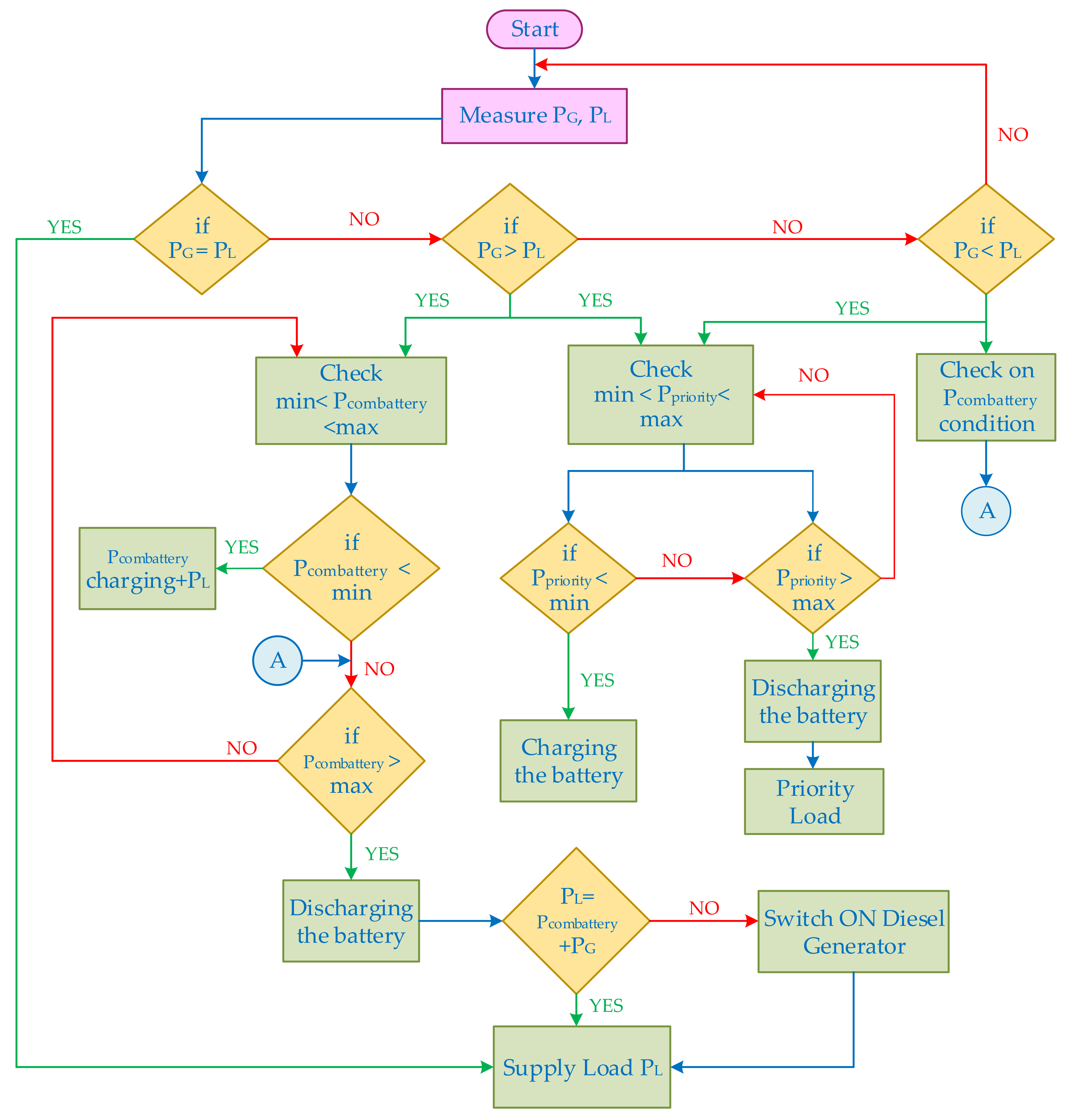
4. Energy Management Strategy

The proposed DC microgrid architecture has three renewable energy sources with the storage device and diesel generator to supply the load continuously. In villages, agriculture is the main occupation of people. Thus, the microgrid is designed to meet the commercial DC and agricultural vehicle load. The lighting of the village will be considered as a priority load in the system. The net generated power and load power P n e t and P L is given by Equations (43) and (44).
P n e t = P P V + P W i n d + P f u e l c e l l
P L = P D L + P A G L + P P L
where,
  • P P V = power generated by PV (kW);
  • P w i n d = power generated by Wind (kW);
  • P f u e l c e l l = power generated by Fuel cell (kW);
  • P L = Domestic load (kW);
  • P A G L = Agriculture vehicle load (kW);
  • P P L = Priority load (kW).
The priority battery is used to supply the lighting load.It will charge during the day and discharge during the night. The generated power will supply the loads by the three cases with the help of the battery and diesel generator. The process is represented as a flow chart in Figure 8. First, the load demand and generated by various sources will be measured based on the condition as follows
• Case 1: Generated power equal to total load.
In this condition, the power generated by wind, PV, and fuel cell is equal to the total load, hence the load will be supplied by the generation without any interruption.
• Case 2: Generated power higher than the load.
In this case, the generated power is higher than the load, hence the renewable power is fully supplied to the required load. The excess power from the generation is charged to the battery. The proposed architecture has two batteries: one is the priority load battery, and the other is the domestic and agricultural load side battery.While the load is supplied, at the same time, the priority battery SoC will be checked. Thus, the condition of priority the load battery and domestic load battery is discussed in Case 3 and Case 4.
• Case 3: Priority load battery charging.
In this case, the SoC of the priority load battery is measured. If the priority is minimum, the battery is charged until it reaches the rate power on that interval. Once it reaches the rated power, the priority battery will not charge, and the excess power generated by the energy source will charge the commercial battery.
S o C m i n < S o C p r i o r i t y < S o C m a x
P p o w e r > P r a t e d = c h a r g i n g
P p o w e r < P r a t e d = d i s c h a r g i n g
P p r i o r i t y = { 7   a . m .   < c h a r g i n g   < 6   p . m .     rated   ( kW / h ) 6   p . m .   < d i s c h a r g i n g   < 7   a . m .   rated   ( kW / h ) }
where, P p o w e r = priority load power P r a t e d = rated (kW/h) to be charged on the condition of P p r i o r i t y interval, charging on daytime P r a t e d = rated (kW/h) to be discharged on the condition of P p r i o r i t y interval discharging on night time.
• Case 4: Domestic and agricultural charging.
In this case, the SoC of the commercial load battery is measured, if the SoCCombattery is minimized then the battery is charged till the SoC of the battery reaches the maximum value. Once it is fully charged excess power generated will be reduced by controlling the output of the fuel cell.
S o C m i n < S o C C o m b a t t e r y < S o C max
S o C C o m b a t t e r y > S o C m i n = c h a r g i n g
S o C C o m b a t t e r y > S o C max = d i s c h a r g i n g
• Case 5: PG < PL.
The generated power will be less than the required load, in this case. This case will be treated with caution to supply the load with the help of the battery by cases 6 and 7. Whatever the load profile may be, the priority load will be supplied by generation, which is the major consideration in this case. The difference in power from the generation and load will be calculated, and then whether the available generation is enough to meet the priority load will be checked. When the condition is satisfied, the priority load will be met by the available generation.
Pmin < Ppriority < Pmax
Pnet = Pmin > Prated (i.e., checks the condition for the case 6)
Pnet = Pmax < Prated Supply the load
• Case 6: Checking the condition of commercial battery PCombattery.
In this case, the commercial load battery power is measured.The generated power and the commercial load battery are checked to see if they are able to supply the load. If the power is sufficient, the demand will be supplied until the SoC of the commercial load battery reaches a minimum level.
SoCmin < SoCCombattery < SoCmaxSoC for the commercial battery
SoCCombattery < SoCmax Battery is discharging
PL = PCombattery + PG
• Case 7: Checking the total demand with respect to the generator.
If PL = PCombattery + PG, then the demand will be supplied through the diesel generator, and the system will continuously check the generative power and the priority load. Once the generation power is enough to supply the load, the diesel generator is cut off from the grid.This process is continued to give uninterrupted power to consumers in remote villages.
P L = P c o m b a t t e r y + P G + P D i e s e l

5. Simulation Study and Results

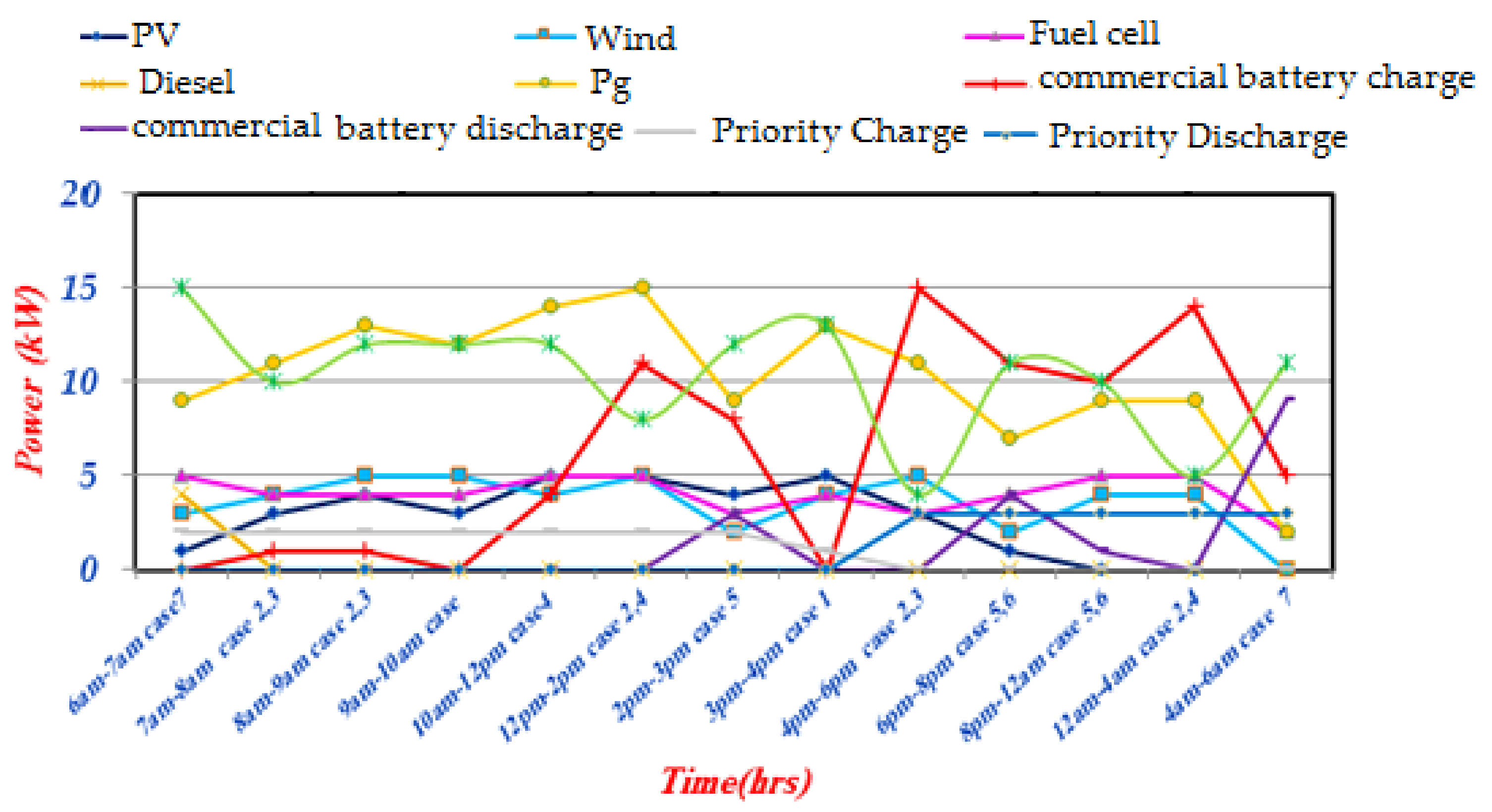
5.1. Simulation Results

The proposed EMS is simulated for the DC microgrid using MATLAB/Simulink. The simulation parameters are shown in Table 1. The control parameter for the EMS is PV, wind, fuel cell, battery, diesel generator, and load power. The load is subdivided into three categories: priority, commercial, and agricultural vehicle load.
The priority load consists of the basic requirement of load that has to be supplied continuously (street lighting of village community), whereas the commercial load and agricultural vehicle load vary according to the requirements of the consumer. Based on the available power generated by all sources with respect to load, the EMS is categorized into the following three cases:
  • Generation equal to load (PG = PL);
  • Generation greater than load (PG > PL);
  • Generation less than load (PG < PL).

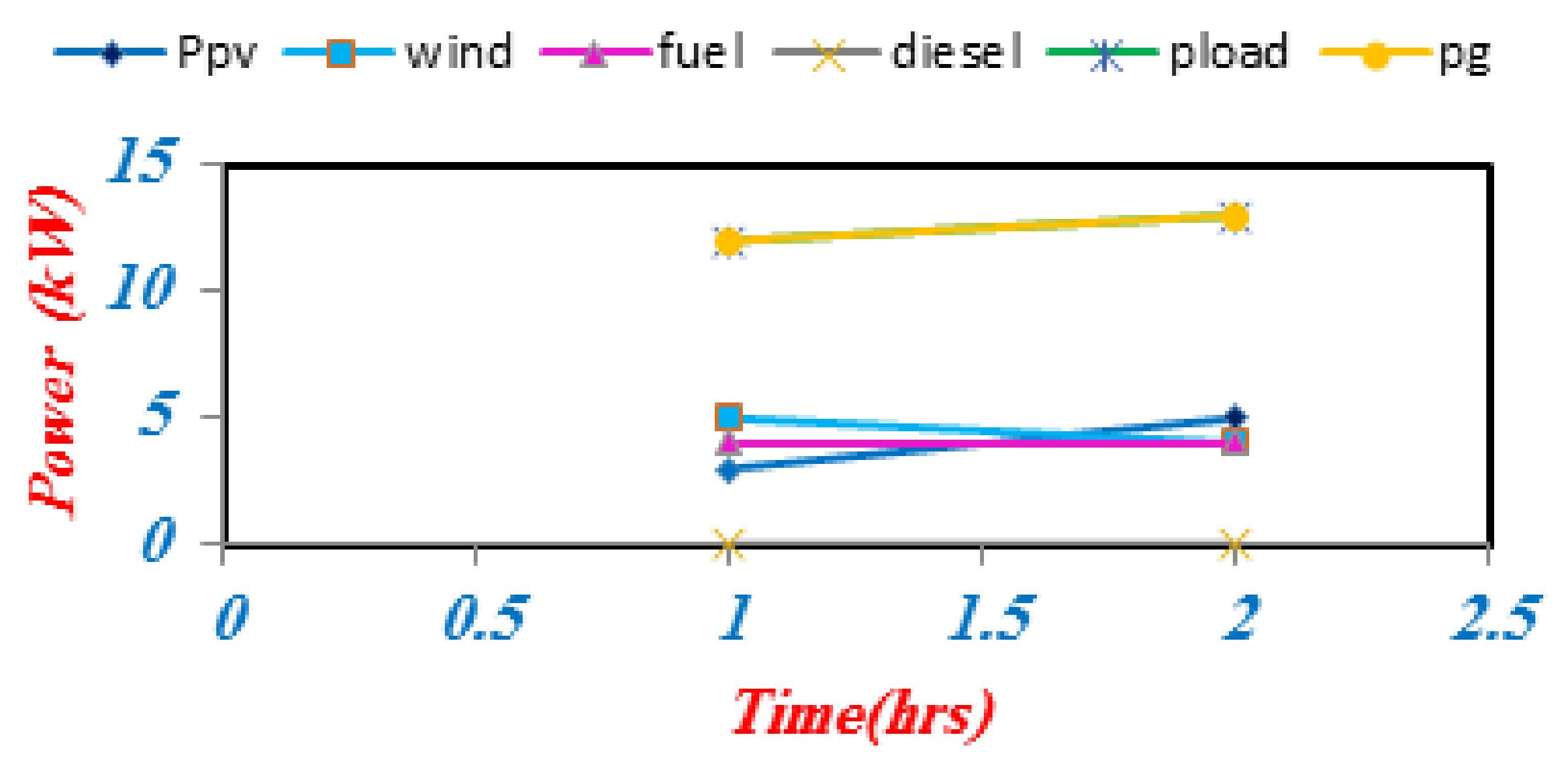
5.2. Generation Equal to Load (PG = PL)

The characteristic curve shown in Figure 9 illustrates that the available power generation is equal to the load condition that is plotted between times versus power. From this condition, the renewable power energy source power is completely utilized to meet the demand requirements.In this condition, the battery will not charge/discharge because the power is deficient. It will not be necessary to use the diesel generator in this case. This case only occurs during a few hours a day, which is shown in Table 2.

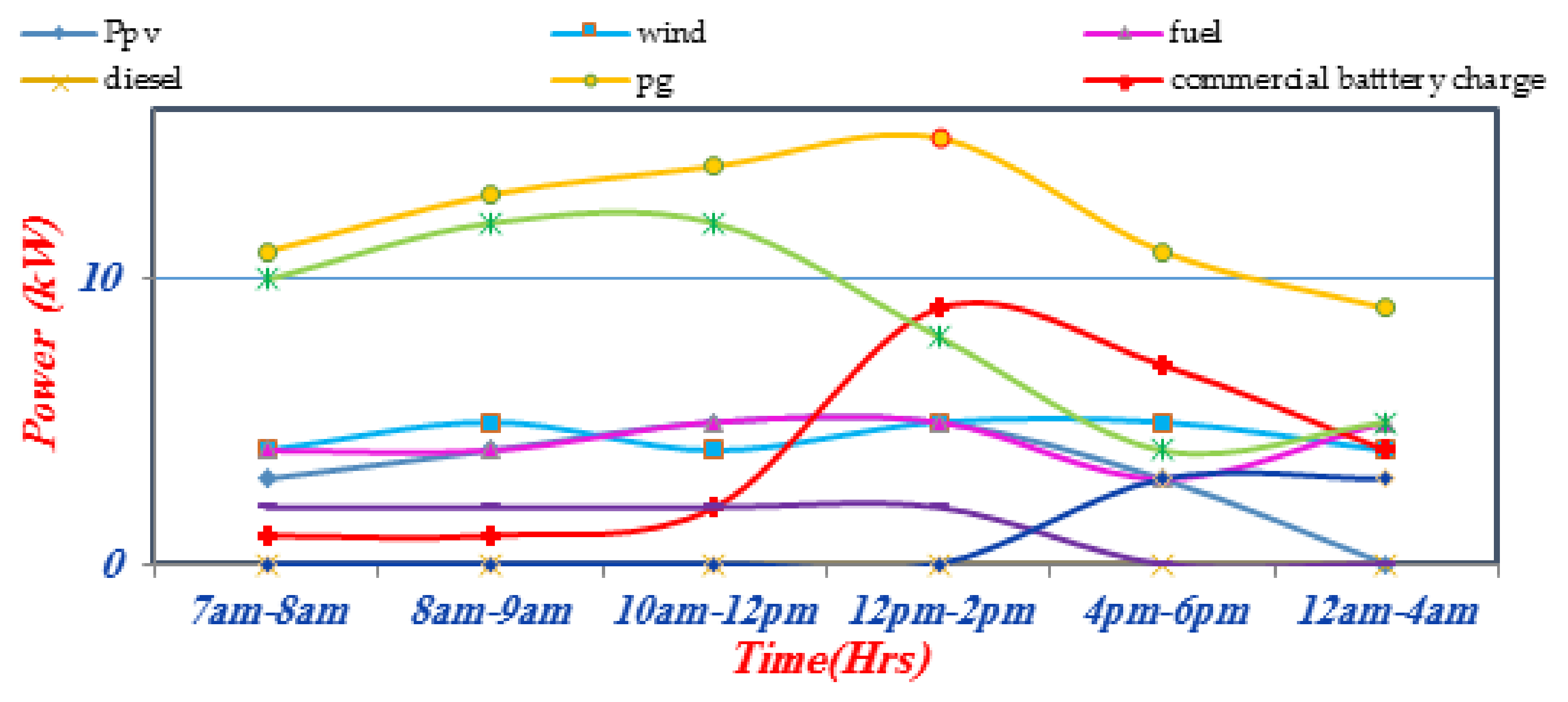
5.3. Generation Greater Than Load (PG > PL)

The Figure 10 shows that the available power generation is greater than load. When PG > PL, the available power is supplied to the consumers and excess power is stored in batterries. However, before storing energy in the batteries, the EMS checks the SoC of both the batteries. First, the priority load battery SoC will be checked and be based on the requirement in a particular interval. It will be charged, and next, the load-side battery SoC will be measured based on the level of SoC. When the SoC is minimized, the power is not delivered to the load; rather, it is stored in the batteries. In certain cases, the power will be extremely high and the load is quite low.Then, the battery is charged completely. There will be surplus power.Thus, the generation of power is cutoff.

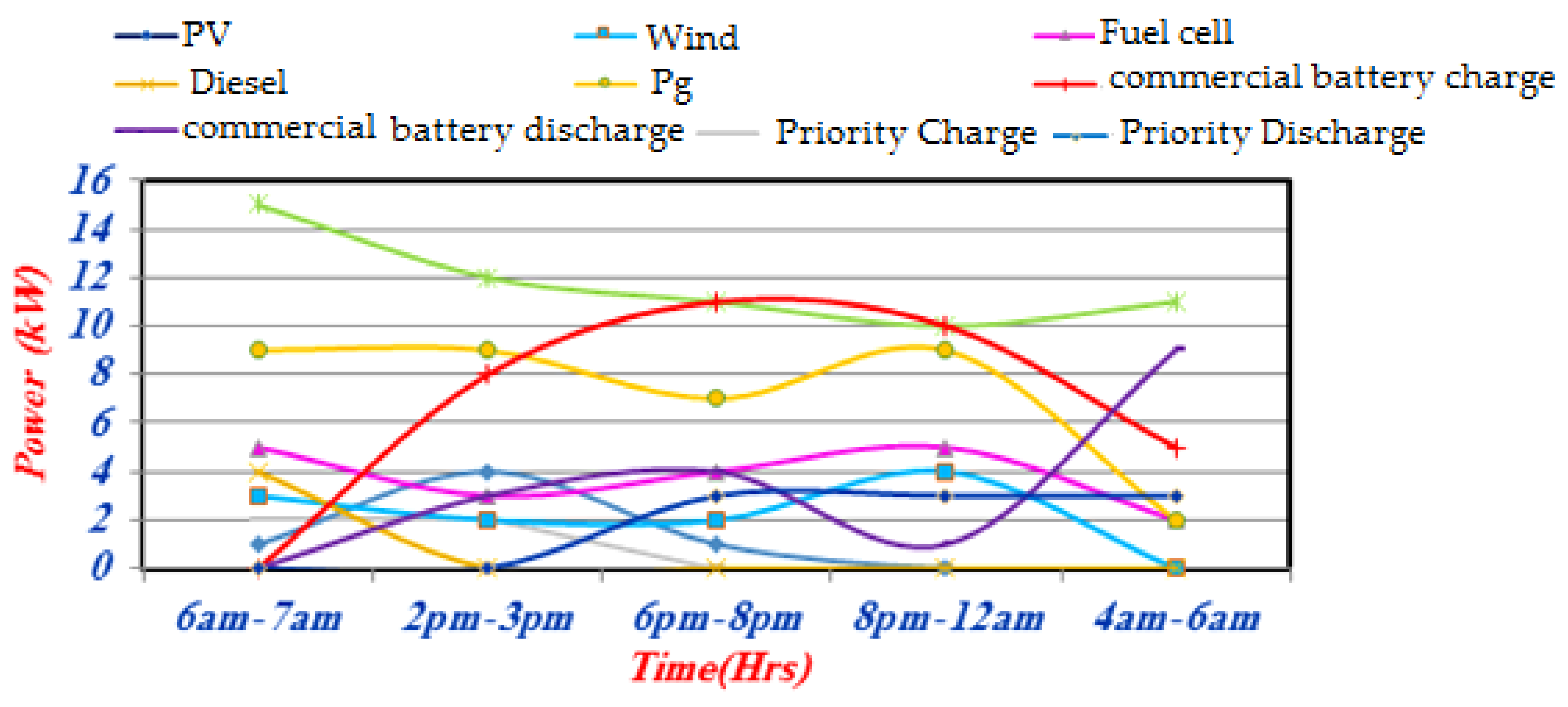
5.4. Generation Greater Than Load (PG < PL)

Figure 11 illustrates the condition where the available power generated is less than the load. During (PG < PL), the EMS checks whether the power generated is able to supply at least the priority load or not. If the generated power is sufficient to supply the demand of priority load, the EMSthen checks the condition of the battery. The priority load will be supplied by the generators. For supplying the commercial and agricultural vehicle load, the battery will supply power when the required power is already stored in the battery. If the battery power and generated power is not able to supply the load, the diesel generator will then supply the load power. The performance of the proposed EMS is analyzed for a 24 h period, which is shown in Table 2. From that table, it is observed that the load requirement of the rural village community is supplied by the penetration of various renewable energy sources rather than the diesel generator. The diesel consumption of the DC microgrid is only 4 kW for one hour in a whole day compare to all other EMS.
The complete performance of the proposed system for 24 h period of the EMS of the DC microgrid is summarized in Table 3, and Figure 12 describes the PV, wind, fuel cell, and diesel power and their operating condition with respect to load in all cases. The laboratory-scale DC microgrid has a capacity of 750 W, and with each renewable energy source, the capacity is 250 W.The performance of all the sources depends on the climatic condition. The power upstream and downstream of the DC microgrid depends on the maximum and minimum voltage, current rating, with respect to the standard test condition (STC) of individual sources stated by the manufacturer. Based on that, the DC microgrid is designed, and their specification is described in Table 4.

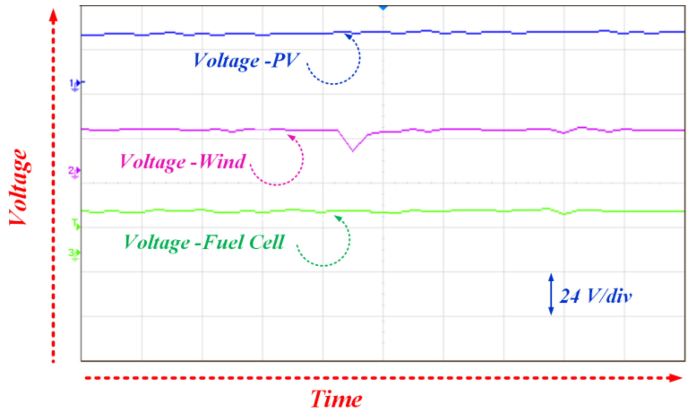
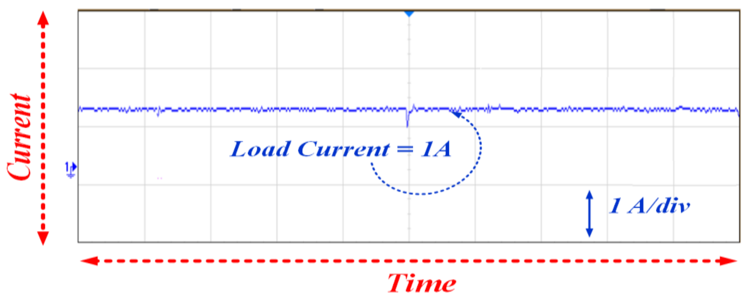
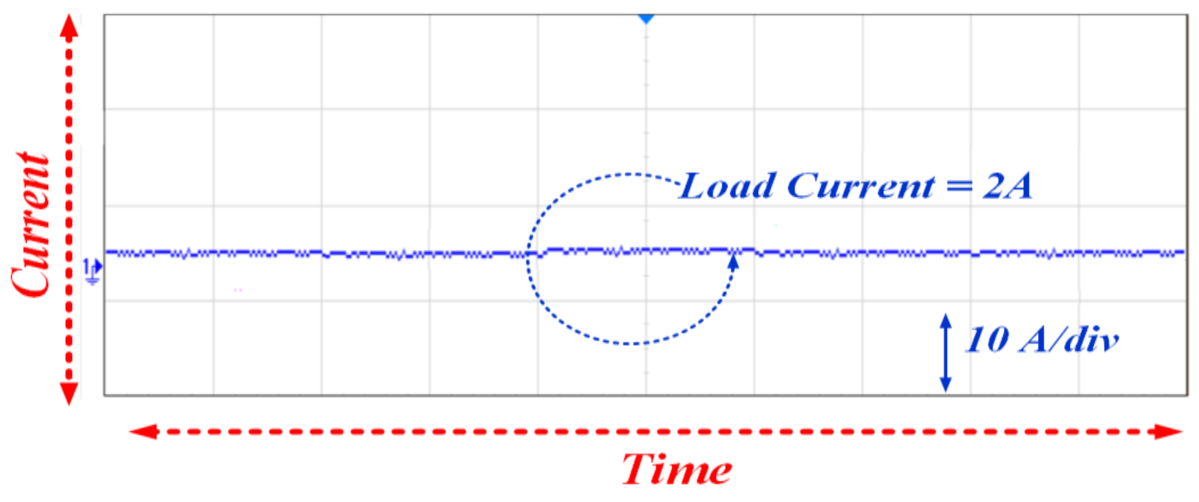
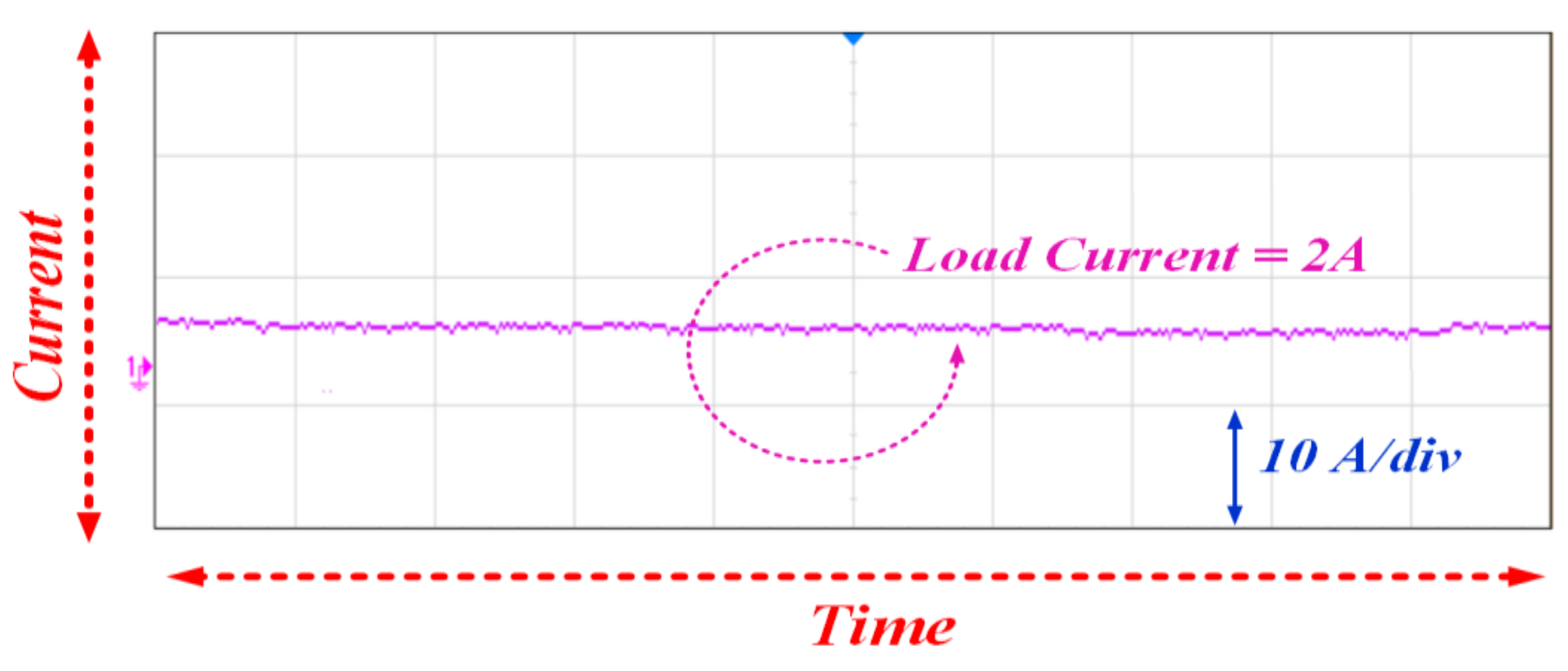
6. Experimental Analysis

The performance of the proposed EMS is verified by the laboratory-scale DC microgrid. The output power of the PV and fuel cell are DC, but for output power is AC.Thus, the AC power is converted to DC with the help of converters. All three sources are integrated to a common DC bus, and a charge controller is used to maintain the voltage level. Two batteries are connected in parallel to supply the demand. One is the priority load battery, and the other is the commercial load battery. The charging and discharging modes of the batteries are based on the availability of power in the DC microgrid. The hardware description for the DC microgrid is presented in Table 5.
The common DC bus voltage of the laboratory scale system is 24 V, and the 24 V/220 V converter is used to maintain the voltage level at load bus. The EMS is tested under the following cases:
  • P G > P L
  • P G = P L
  • P G < P L
The EMS continuously monitors the load power with respect to the renewable power generation. Based on its performance, the DC microgrid will supply the load. Two types of loads are considered to validate the performance: one is the priority load, and the other is the commercial load.
The priority load is the lighting load that will charge during the day and discharge at night. The commercial battery is charged based on the availability of RES with respect to the load. The experimental results are shown in Table 6.
(1) Case 1: P G > P L
During 7 a.m.–8 a.m., the total power generated from the REG is 370 W. At that instant, the demand is 250 and the load current is 1.2Amps. The excess power (120 W) is stored in the commercial load battery. The voltage of the DC bus and the load current waveform is shown in Figure 13 and Figure 14.
(2) Case 2: P G = P L
When the load is raised at 9 a.m.–10 a.m. to generate power, the load power is 440 W and the load current is 2 A, and the generated power continuously supplies the load without any interruption. At that interval, the commercial battery is in standby mode (no charging and discharging). The load current and priority load battery charging waveform are shown in Figure 15 and Figure 16.
(3) Case 3: P G < P L
Normally, PV does not supply power from 6 p.m.–6 a.m. due to the sun irradiation portfolio. During this time, the rest of power sources (wind and fuel cell) combine with battery to supply the load. At 8 p.m.–12 a.m., the load is considered to be 900 W and the available generation is 600 W. In this case, the microgrid power demand is satisfied through a combination of battery and available energy sources (wind and fuel cell). The load current, commercial load battery, and priority load battery charging waveform are shown in Figure 17 and Figure 18. If the total generation on the microgrid is low when compared to the load, the diesel generator will switch on to supply the load until the renewable power becomes active. From all the three cases, this system will be reliable and supply the load without any interruption. The main advantage of this DC micro grid is that it will supply the load to the consumer with the depth penetration of renewable energy sources rather than the diesel generator. It is concluded that the prototype of the 500 W microgrid is tested and validated with different conditions. The results satisfy the EMS for both the simulation and the hardware setup. The DC microgrid architecture is scalable for 15 kW to satisfy the load demand in rural communities.

7. Conclusions

In this paper, an EMS is proposed for different renewable sources fedtoDC microgrid for remote village communities with capricious load conditions. The Proposed DC microgrid handles the load power balancing for DG sources based on EMS. The proposed system is applicable for electrifying rural communities with maximum penetration of renewable energy sources and storage systems. Furthermore, this EMS is able to handle the load–power balancing for all the capricious cases (PG = PL, PG > PL and PG < PL) and providesa continuously supply to rural communities (described in Table 2 for all capricious cases). The load–power balancing is performed based on two battery sources: one is the priority battery (which handles the priority load), and the other is the commercial battery (which isapplicable to common DC bus). This battery is able to handle the load demand for various capricious cases, which are described in Table 2. Hence, the EMS utilizes the maximum power from the renewable sources and reduces the consumption of non-conventional energy sources (a diesel generator). The simulation and experimental studies of the DC microgrid with the proposed EMS clearly indicates that the power dissipates to the consumer through maximum renewable energy penetration and batteries throughout the day without any divergence in the system. Thus, the proposed EMS is verified through a laboratory-scale real time DC microgrid experimental setup and confirms its merits.

Author Contributions

Maheswaran Gunasekaran and Hidayathullah Mohamed Ismail has developed the proposed research concept, and they both are involved to study the execution and implementation with numerical software by collecting information from the real environment and developed the simulation model for the same. Maheswaran Gunasekaran has implemented the proposed concept in laboratory prototype environment with Bharatiraja Chokkalingam. Sanjeevikumar Padmanaban, and Lucian Mihet-Popa shared thier expertise and validation examinations to confirm the concept theoretically with the obtained numerical results for its validation of the proposal. All authors Maheswaran Gunasekaran, Hidayathullah Mohamed, Bharatiraja Chokkalingam, Sanjeevikumar Padmanaban, Lucian Mihet-Popa, involved to frame the final version of the manuscript as a full research article. Moreover, all authors involved in validating and to make the article error free technical outcome for the set investigation work.

Conflicts of Interest

The authors declare no conflict of interest.

References

  1. Bloomberg New Energy Finance. The Future of Energy 2012 Results Book; Bloomberg New Energy Finance: New York, NY, USA, 2012. [Google Scholar]
  2. International Energy Agency World Energy Investment. Available online: https://www.iea.org/media/publications/investment/WEI2017Launch_forWEB.pdf (accessed on 10 April 2017).
  3. Anand, S.; Fernandes, B.G. Steady state performance analysis for load sharing in DC distributed generation system. In Proceedings of the 2011 10th International Conference on Environment and Electrical Engineering (EEEIC), Rome, Italy, 8–11 May 2011; pp. 1–4. [Google Scholar]
  4. Gao, L.; Liu, Y.; Ren, H.; Guerrero, J.M. A DC Microgrid Coordinated Control Strategy Based on Integrator Current-Sharing. Energies 2017, 10, 1116. [Google Scholar] [CrossRef]
  5. Patterson, B.T. Dc, come home: Dc microgrids and the birth of the ‘enernet’. IEEE Power Energy Mag. 2012, 10, 60–69. [Google Scholar] [CrossRef]
  6. Ali, A.; Padmanaban, S.; Twala, B.; Marwala, T. Electric Power Grids Distribution Generation System for Optimal Location and Sizing—A Case Study Investigation by Various Optimization Algorithms. Energies 2017, 10, 960. [Google Scholar] [CrossRef]
  7. Liu, X.; Wang, P.; Loh, P.C. A hybrid AC/DC microgrid and its coordination control. IEEE Trans. Smart Grid 2011, 2, 278–286. [Google Scholar] [CrossRef]
  8. Sechilariu, M.; Wang, B.C.; Locment, F. Supervision control for optimal energy cost management in DC microgrid: Design and simulation. Int. J. Electr. Power Energy Syst. 2014, 58, 140–149. [Google Scholar] [CrossRef]
  9. Hossain, E.; Perez, R.; Padmanaban, S.; Mihet-Popa, L.; Blaabjerg, F.; Ramachandaramurthy, V.K. Sliding Mode Controller and Lyapunov Redesign Controller to Improve Microgrid Stability: A Comparative Analysis with CPL Power Variation. Energies 2017, 10, 1959. [Google Scholar] [CrossRef]
  10. Subramani, G.; Ramachandaramurthy, V.K.; Padmanaban, S.; Mihet-Popa, L.; Blaabjerg, F.; Guerrero, J.M. Grid-Tied Photovoltaic and Battery Storage Systems with Malaysian Electricity Tariff—A Review on Maximum Demand Shaving. Energies 2017, 10, 1884. [Google Scholar] [CrossRef]
  11. Tan, K.M.; Ramachandaramurthy, V.K.; Yong, J.Y.; Padmanaban, S.; Mihet-Popa, L.; Blaabjerg, F. Minimization of Load Variance in Power Grids—Investigation on Optimal Vehicle-to-Grid Scheduling. Energies 2017, 10, 1880. [Google Scholar] [CrossRef]
  12. Sen, R.; Bhattacharyya, S.C. Off-grid electricity generation with renewable energy technologies in India: An application of HOMER. Renew. Energy 2014, 62, 388–398. [Google Scholar] [CrossRef]
  13. AL-Nussairi, M.K.; Bayindir, R.; Padmanaban, S.; Mihet-Popa, L.; Siano, P. Constant Power Loads (CPL) with Microgrids: Problem Definition, Stability Analysis and Compensation Techniques. Energies 2017, 10, 1656. [Google Scholar] [CrossRef]
  14. Ganesan, S.; Padmanaban, S.; Varadarajan, R.; Subramaniam, U.; Mihet-Popa, L. Study and Analysis of an Intelligent Microgrid Energy Management Solution with Distributed Energy Sources. Energies 2017, 10, 1419. [Google Scholar] [CrossRef]
  15. Song, M.; Chen, K.; Zhang, X.; Wang, J. Optimization of wind turbine micro-siting for reducing the sensitivity of power generation to wind direction. Renew. Energy 2016, 85, 57–65. [Google Scholar] [CrossRef]
  16. Dixon, C.; Reynolds, S.; Rodley, D. Micro/small wind turbine power control for electrolysis applications. Renew. Energy 2016, 87, 182–192. [Google Scholar] [CrossRef]
  17. Macedo, W.N.; Monteiro, L.G.; Corgozinho, I.M.; Macêdo, E.N.; Rendeiro, G.; Braga, W.; Bacha, L. Biomass based microturbine system for electricity generation for isolated communities in amazon region. Renew. Energy 2016, 91, 323–333. [Google Scholar] [CrossRef]
  18. Chokkalingam, B.; Padmanaban, S.; Siano, P.; Krishnamoorthy, R.; Selvaraj, R. Real-Time Forecasting of EV Charging Station Scheduling for Smart Energy Systems. Energies 2017, 10, 377. [Google Scholar] [CrossRef]
  19. Bonfiglio, A.; Brignone, M.; Invernizzi, M.; Labella, A.; Mestriner, D.; Procopio, R. A Simplified Microgrid Model for the Validation of Islanded Control Logics. Energies 2017, 10, 1141. [Google Scholar] [CrossRef]
  20. Long, B.; Jeong, T.W.; Deuk Lee, J.; Jung, Y.C.; Chong, K.T. Energy management of a hybrid AC–DC micro-grid based on a battery testing system. Energies 2015, 8, 1181–1194. [Google Scholar] [CrossRef]
  21. Martin-Martínez, F.; Sánchez-Miralles, A.; Rivier, M. A literature review of Microgrids: A functional layer based classification. Renew. Sustain. Energy Rev. 2016, 62, 1133–1153. [Google Scholar] [CrossRef]
  22. Shahzad, M.K.; Zahid, A.; Ur Rashid, T.; Rehan, M.A.; Ali, M.; Ahmad, M. Techno-economic feasibility analysis of a solar-biomass off grid system for the electrification of remote rural areas in Pakistan using HOMER software. Renew. Energy 2017, 106, 264–273. [Google Scholar] [CrossRef]
  23. Olatomiwa, L.; Mekhilef, S.; Ismail, M.S.; Moghavvemi, M. Energy management strategies in hybrid renewable energy systems: A review. Renew. Sustain. Energy Rev. 2016, 62, 821–835. [Google Scholar] [CrossRef]
  24. Mandelli, S.; Barbieri, J.; Mereu, R.; Colombo, E. Off-grid systems for rural electrification in developing countries: Definitions, classification and a comprehensive literature review. Renew. Sustain. Energy Rev. 2016, 58, 1621–1646. [Google Scholar] [CrossRef]
  25. Hosseini, S.A.; Abyaneh, H.A.; Sadeghi, S.H.H.; Razavi, F.; Nasiri, A. An overview of microgrid protection methods and the factors involved. Renew. Sustain. Energy Rev. 2016, 64, 174–186. [Google Scholar] [CrossRef]
  26. Jing, W.; Lai, C.H.; Wong, S.H.W.; Wong, M.L.D. Battery-supercapacitor hybrid energy storage system in standalone DC microgrids: A review. IET Renew. Power Gener. 2016, 11, 461–469. [Google Scholar] [CrossRef]
  27. Kinhekar, N.; Padhy, N.P.; Li, F.; Gupta, H.O. Utility oriented demand side management using smart AC and micro DC grid cooperative. IEEE Trans. Power Syst. 2016, 31, 1151–1160. [Google Scholar] [CrossRef]
  28. Gabbar, H.A.; Othman, A.M. Performance optimisation for novel green plug-energy economizer in micro-grids based on recent heuristic algorithm. IET Gener. Transm. Distrib. 2016, 10, 678–687. [Google Scholar] [CrossRef]
  29. Ackermann, T.; Cherevatskiy, S.; Brown, T.; Eriksson, R.; Samadi, A.; Ghandhari, M.; Söder, L.; Lindenberger, D.; Jägemann, C.; Hagspiel, S.; et al. Smart Modeling of Optimal Integration of High Penetration of PV-SMOOTH PV. Available online: http://smooth-pv.info/doc/SmoothPV_Final_Report_Part1.pdf. (accessed on 19 January 2018).
  30. Arboleya, P.; Gonzalez-Moran, C.; Coto, M.; Falvo, M.C.; Martirano, L.; Sbordone, D.; Bertini, I.; Di Pietra, B. Efficient energy management in smart micro-grids: ZERO grid impact buildings. IEEE Trans. Smart Grid 2015, 6, 1055–1063. [Google Scholar] [CrossRef]
  31. Chub, A.; Husev, O.; Blinov, A.; Vinnikov, D. Novel Isolated Power Conditioning Unit for Micro Wind Turbine Applications. IEEE Trans. Ind. Electron. 2017, 64, 5984–5993. [Google Scholar] [CrossRef]
  32. RRahman, S.A.; Varma, R.K.; Vanderheide, T. Generalised model of a photovoltaic panel. IET Renew. Power Gener. 2014, 8, 217–229. [Google Scholar] [CrossRef]
  33. Silva, E.A.; Bradaschia, F.; Cavalcanti, M.C.; Nascimento, A.J. Nascimento. Parameter estimation method to improve the accuracy of photovoltaic electrical model. IEEE J. Photovolt. 2016, 6, 278–285. [Google Scholar] [CrossRef]
  34. Bhayo, M.A.; Yatim, A.H.M.; Khokhar, S.; Aziz, M.J.A.; Idris, N.R.N. Modeling of Wind Turbine Simulator for analysis of the wind energy conversion system using MATLAB/Simulink. In Proceedings of the IEEE Conference on Energy Conversion (CENCON), Johor Bahrum, Malaysia, 19–20 October 2015; pp. 122–127. [Google Scholar]
  35. Breaz, E.; Gao, F.; Blunier, B.; Tirnovan, R. Mathematical modeling of proton exchange membrane fuel cell with integrated humidifier for mobile applications. In Proceedings of the IEEE Transportation Electrification Conference and Expo (ITEC), Dearborn, MI, USA, 18–20 June 2012; pp. 1–6. [Google Scholar]
  36. Mihet-Popa, L.; Boldea, I. Dynamics of control strategies for wind turbine applications. In Proceedings of the 10th International Conference on Optimisation of Electrical and Electronic Equipment, OPTIM 2006, Poiana Brasov, Romania, 18−19 May 2006; pp. 199–206. [Google Scholar]
  37. Yu, S.Y.; Kim, H.J.; Kim, J.H.; Han, B.M. SoC-based output voltage control for BESS with a lithium-ion battery in a stand-alone DC microgrid. Energies 2016, 9, 924. [Google Scholar] [CrossRef]
  38. Zhou, N.; Liu, N.; Zhang, J.; Lei, J. Multi-Objective optimal sizing for BATTERY Storage of PV-based microgrid with demand response. Energies 2016, 9, 591. [Google Scholar] [CrossRef]
  39. Mihet-Popa, L.; Camacho, O.M.F.; Norgard, P.B. Charging and discharging tests for obtaining an accurate dynamic electro-thermal model of high power lithium-ion pack system for hybrid and EV applications. In Proceedings of the IEEE PES Power Tech Conference, Grenoble, France, 16−20 June 2013. [Google Scholar]
  40. Camacho, O.M.F.; Mihet-Popa, L. Fast Charging and Smart Charging Tests for Electric Vehicles Batteries using Renewable Energy. Oil Gas Sci. Technol. 2016, 71, 13. [Google Scholar] [CrossRef]
Figure 1. Power system network.
Applsci 08 00585 g001
Figure 2. Proposed DC microgrid architecture.
Applsci 08 00585 g002
Figure 3. A single diodemodel of a photovoltaic (PV) cell.
Applsci 08 00585 g003
Figure 4. Solar cell characteristics curve (voltage vs. current and power).
Applsci 08 00585 g004
Figure 5. Characteristic curve of wind system (wind speed vs. power).
Applsci 08 00585 g005
Figure 6. Equivalent circuit of the fuel cell.
Applsci 08 00585 g006
Figure 7. Single fuel cell characteristics curve (stack current vs. cell voltage and power).
Applsci 08 00585 g007
Figure 8. Flowchart for proposed energy management strategy (EMS) of the DC microgrid.
Applsci 08 00585 g008
Figure 9. Generation is equal to the load (PG = PL) (power vs. time).
Applsci 08 00585 g009
Figure 10. Generation greater than load (PG > PL) (power vs. time).
Applsci 08 00585 g010
Figure 11. Generation greater than load (PG > PL).
Applsci 08 00585 g011
Figure 12. Overall performance of the system with generated power.
Applsci 08 00585 g012
Figure 13. Voltage across each renewable energy source.
Applsci 08 00585 g013
Figure 14. Load current during 7 a.m.–8 a.m.
Applsci 08 00585 g014
Figure 15. Load current during 9 a.m.–10 a.m.
Applsci 08 00585 g015
Figure 16. Load current during 8 p.m.–12 a.m.
Applsci 08 00585 g016
Figure 17. Commercial battery charging/discharging profile.
Applsci 08 00585 g017
Figure 18. Priority load battery charging/discharging profile.
Applsci 08 00585 g018
Table 1. Simulation parameters.
DescriptionSpecification
Wind generator5 kW, 220 V
PV5 kW, 220 V
Fuel Cell5 kW, 220 V
DC bus voltage220 V
DC-DC converter220 V
Dynamic Load5 kW
Motor load2.5 kW to 5 kW
Battery220 V battery/150 Ah
Table 2. Simulated result values (“kW”) of the DC microgrid with EMS.
TimePower Generated by Renewable Energy SourceDiesel PowerTotal Generated PowerCommercial BatteryPriority Load BatteryPriority LoadDomestic LoadsAgricultural LoadsTotal Loads
Ppv (kW)Wind (kW)Fuel (kW)Diesel (kW)Pg (kW)Charge (kW/h)Discharge (kW/h)Charge (kW/h)Discharge (kW/h)Load (kW)Pd1 (kW)Pd2 (kW)Pag1 (kW)Pag2 (kW)PL (kW)
6 a.m.–7 a.m.1354900−202324415
7 a.m.–8 a.m.344011−10−202222210
8 a.m.–9 a.m.454013−10−202124312
9 a.m.–10 a.m.35401200−202403312
10 a.m.–12 p.m.545014−20−202223312
12 p.m.–2 p.m.555015−70−20221308
2 p.m.–3 p.m.4230903−201233312
3 p.m.–4 p.m.54401300−101414313
4 p.m.–6 p.m.353011−9013−311114
6 p.m.–8 p.m.124070423−3432211
8 p.m.–12 a.m.045090123−3132410
12 a.m.–4 a.m.04509−4023−332005
4 a.m.–6 a.m.002020923−3225211
Table 3. Summary of the EMS.
PGPLPPriorityPComPDieselCasesRemarks
1PG = PL×1The power from renewable source is enough to supply the load without storage unit and diesel generator.
2PG > PL×2,3,4The load will be supplied and additionally the batteries will charge with the surplus power
3PG < PL5,6,7The load is supplied by the combination of diesel generator, available power, and battery.
Table 4. Hardware specifications of the proposed DC microgrid.
PVWindFuel Cell
Centsys Solar 250 WSIKCO Wind 1000Horizon 500 W PEM Fuel Cell
PV ModulesSpecificationWindSpecificationFuel CellSpecification
Maximum capacity250 WType of TurbineHorizontal Axis Downwind TurbineRated capacity500 W
Tolerance±3%voltage12 V DCRated voltage14.4 V
Open circuit voltage37.8 VRated Wind Speed5 m/sValve Voltage12 V
Short circuit current7.94 ARated Power300 WBlower range12 V
Module efficiency15.3%Rated rpm300ReactantsHydrogen and Air
Solar cell efficiency17.2%Cut-in wind speed2 m/sAmbient Temperature5–30 °C (41–86 °F)
Maximum voltage (Vm)31.5 VCut-out wind speed15 m/sMax Stack Temperature65 °C (149 °F)
Maximum current (Im)7.94 ABlade length600 mmGas Pressure0.45–0.55 Bar
Nominal Temperature42 °C (±2 °C)blades6Stack Size268 mm × 130 mm × 122.5 mm (10.5″ × 5.1″ × 4.8″)
Dimensions1650 mm × 992 m × 40 mmNoise Level<20 dBEfficiency of System40% at 14.4 V
Table 5. Hardware description of components used.
ParametersSpecification
DC bus voltage24 V
Capacityof wind generator200 W
Capacity of PV panel200 W
Capacity of fuel cell power100 W
Battery typeTall tubular C10
Battery capacity14 Ah/12 V
DC-DC converter24 V/220 V
Lamp loads500 W
Load bus220 V
Diesel generator500 W
Maximum current3 A
Table 6. Experimental results at different time periods.
TimePV Power (W)Wind Power (W)Fuel Cell Power (W)Generated Power (W)Loads (W)Batteries
Priority LoadCommercial LoadsNet LoadsPriority Load BatteryCommercial Load Battery
P(W)I(A)P(W)I(A)P(W)I(A)P(W)I(A)P(W)I(A)P(W)I(A)
7 a.m.–8 a.m.1001701003701.681000.51500.72501.2−100−0.5−120−0.7
9 a.m.–10 a.m.20014010044021000.53401.54402.0−100−0.500
8 p.m.–12 a.m.01501002501.131000.52501.13501.61000.51000.45

