Probabilistic Sensitivity Amplification Control for Lower Extremity Exoskeleton

1
State Key Laboratory of Robotics and System, Harbin Institute of Technology, Harbin 150080, China
2
School of Astronautics, Harbin Institute of Technology, Harbin 150080, China
3
Weapon Equipment Research Institute, China Ordnance Industries Group, Beijing 102202, China
*
Author to whom correspondence should be addressed.
Appl. Sci. 2018, 8(4), 525; https://doi.org/10.3390/app8040525
Submission received: 27 January 2018
/
Revised: 26 March 2018
/
Accepted: 27 March 2018
/
Published: 29 March 2018
Abstract
:To achieve ideal force control of a functional autonomous exoskeleton, sensitivity amplification control is widely used in human strength augmentation applications. The original sensitivity amplification control aims to increase the closed-loop control system sensitivity based on positive feedback without any sensors between the pilot and the exoskeleton. Thus, the measurement system can be greatly simplified. Nevertheless, the controller lacks the ability to reject disturbance and has little robustness to the variation of the parameters. Consequently, a relatively precise dynamic model of the exoskeleton system is desired. Moreover, the human-robot interaction (HRI) cannot be interpreted merely as a particular part of the driven torque quantitatively. Therefore, a novel control methodology, so-called probabilistic sensitivity amplification control, is presented in this paper. The innovation of the proposed control algorithm is two-fold: distributed hidden-state identification based on sensor observations and evolving learning of sensitivity factors for the purpose of dealing with the variational HRI. Compared to the other state-of-the-art algorithms, we verify the feasibility of the probabilistic sensitivity amplification control with several experiments, i.e., distributed identification model learning and walking with a human subject. The experimental result shows potential application feasibility.
1. Introduction
In recent decades, with the dramatic progress in computing, control and sensing, significant types of prostheses, orthoses and exoskeletons have been designed and developed to assist and support human limbs for various tasks. In order to increase the operator’s strength and endurance, the exoskeleton is a typical class of wearable mechatronic robotic systems, which are designed to meet this demand. A particular feature of this kind of exoskeleton is that they are fully driven by the pilot intention and follow the pilot movements in synchrony. The application feasibility includes functional rehabilitation for the injured, physical assistance for the disabled and elderly and fatigue relief for heavy-duty workers. To recognize human intention, two main groups of sensors, i.e., cognitive-based sensors, as well as physical-based sensors, are usually applied to capture the information of the human interaction or the muscle signals.
By measuring the electric signals from the musculoskeletal system or the nervous system, the operator’s intention read by the cognitive-based sensors can be interpreted as the input to the exoskeleton system controller. A successful practical application of these kinds of exoskeletons is the hybrid assistive limb (Tsukuba University and Cyberdyne, Japan) [1,2], which is structured for whole-body assistance. The muscular activity signal is collected using surface electromyography (sEMG) sensors. In addition, the exploration for brain-machine interface (BMI) control is implemented at the University of Tubingen in Germany [3]. The hybrid BMI system consists of an EMG continuous decoder, as well as an electroencephalogram (EEG) binary classifier. Consequently, the crucial advantage of cognitive-based sensors is that the pilot or the patient intention can still be read, even if the subject cannot provide necessary joint torques. Thus, these types of the sensor systems are widely utilized in rehabilitation and medical application.
An alternative sensor system recognizes the human intentions by applying physical-based sensors. The Body Extender [4] is designed to handle and transport heavy loads up to 100 kg. Consequently, the human intentions are read by the force sensors mounted on the interaction part between the pilot and exoskeleton. The velocity input to the controller is converted by the impedance control algorithm [5,6]. Moreover, for low impedance, back drivability and precise control, a compact rotary series elastic actuator is designed in [7] to fulfill these requirements. The input to the system controller is derived from the deformation of the series elastic module. Also note that an improvement of system stability is introduced in [8], which addresses the time-delay effect of the series elastic module.
Apart from the sensor-based human intention recognition, the sensitivity amplification control is proposed in [9,10] for the Berkeley Lower Extremity Exoskeleton. The design conception of control algorithm aims to enable a pilot’s locomotion with little effort on any type of terrain. In addition, the control scheme demands on interaction sensors between the pilot, as well as the exoskeleton. Nevertheless, the controller has little robustness to model uncertainties or parameter variations.
Although the sensors mounted between the pilot and the exoskeleton can simplify the control algorithm, a crucial issue that should be addressed is that the time-delay effect cannot be avoided. Consequently, the control performance is limited due to this issue, even if the robustness can be enhanced by the compensation of the disturbance observer [11] or the internal model control [12]. The problem of time-delay effect may be solved by the cognitive-based sensors [13,14], since the human intention can be acquired before the movement primitives. Nevertheless, these signals derived from the sensors suffer from unwanted noise, as well as the overlap of the spectrum with other signals.
The sensitivity amplification control (SAC) control scheme has provided a solution for the human performance augmentation exoskeletons. However, such an algorithm suffers from weak robustness, and it barely destroys the control system. Thus, a sophisticated identification process is required to improve system stability, as detailed in [15]. The second drawback is that the fixed sensitivity factor cannot manage the uncertainties of the interaction model.
In this paper, we retain the advantages of the SAC control scheme and propose a novel control scheme, so-called probabilistic sensitivity amplification control, to address the two crucial issues, as shown in Figure 1. Rather than identifying the system dynamics, we infer the state-space model based on a novel distributed identification process. To address the challenge of dealing with the uncertainties of the interaction model, an online reinforcement learning algorithm based on the derandomized evolution strategy with covariance matrix adaptation (CMA-ES) is presented for the adaptation of sensitivity factors. Thus, the sensitivity factors can be effectively updated in a constraint domain of interest according to the torque tracking error penalty.
The remainder of the paper is organized as follows:
After the Introduction, Section 2 is devoted to outlining the main routine of our proposed distributed hidden-state identification to address the issue of weak robustness. In Section 3, the novel evolving learning of sensitivity factors is presented to deal with the variational HRI. The implementation of the experiments and the comparison of the control algorithms are presented in Section 4. Finally, Section 5 concludes with a summary.
2. Distributed Hidden-State Identification
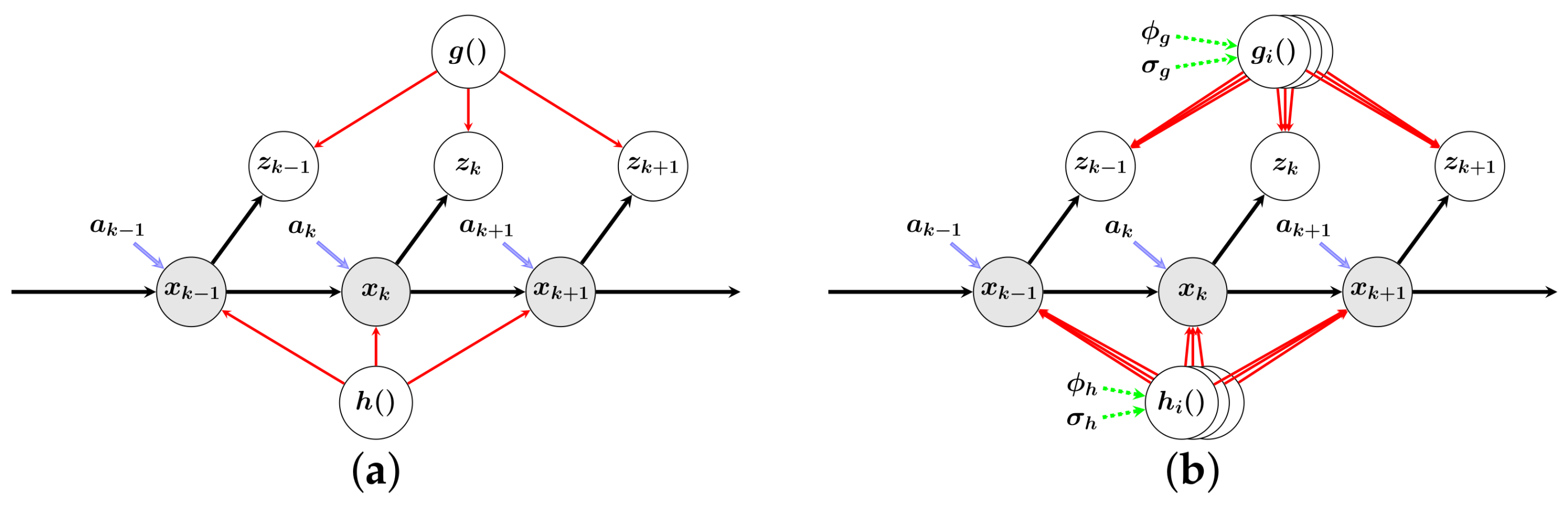
For realizing efficient control of the exoskeleton, it is essential to understand the human intention. According to our control scheme, the intention can be interpreted as the system state variables. Although tremendous attention has been paid to filtering and smoothing [16,17,18], these algorithms do not focus on the identification process, but on inference. In addition, the Gaussian process (GP) state-space model presented in [19] has not addressed the crucial issue of computation expense, which we will carefully discuss in this section. Therefore, the graphic explanation of the crucial difference between the GP state-space inference [17,18,19] and our proposed distributed hidden-state identification are shown in Figure 2.
In this section, firstly, we give a comprehensive explanation of the distributed model learning for the identification process based on the expectation maximization. Then, we introduce the online inference under a distributed framework and Markov chain Monte Carlo, also along with the fusion method, so-called generalized product-of-expert (PoE).
2.1. Model Learning
Although the Gaussian process has a substantial impact in many fields, the crucial limit is that the computation expense scales in for training, while regarding prediction, the computed expense is if caching the kernel matrix. Thus, we employ the distributed Gaussian process [20] to address this issue, since this method can handle arbitrarily large datasets with sufficient hierarchical product-of-expert (PoE) models.
The Gaussian process, fully specified by a mean function and a covariance function , is a probabilistic distribution over functions f. The latent function can be learned from a training dataset , where and . In addition, the posterior predictive distribution of the function by a given set of hyper-parameters is defined with mean and covariance, respectively
With defining input, and . Note that the hyper-parameters of the covariance function consist of the length-scale , the signal variance and the noise variance . Besides, the hyper-parameters are of significance to the covariance function defining the non-parametric model behavior [21].
According to the independent distributed assumption, the marginal likelihood can be decomposed into M individual products:
With M the total number of experts. In the model learning process, the hyper-parameters are shared for all M GPs. Moreover, a usual method for optimizing the hyper-parameters is to maximize the evidence maximization. Nevertheless, we apply a more efficient method in this paper, i.e., expectation maximization with Monte Carlo sampling.
Therefore, the general class of latent state-space models with the Gaussian process is given below:
With . The is a latent state that evolves over time, while can be read from actual measurement data. Both additive system noise, as well as measurement noise are assumed i.i.d. If not stated otherwise, both the measurement function and dynamic function are implicit, but instead can be described with the probability distributions over these Gaussian functions. Here, the functions are a Gaussian process non-parametric model, defined as and , separately.
Limited by the space of this paper, we briefly explain the learning process of the dynamic function . In the expectation step, we compute the posterior distribution of the system states , where and . Nevertheless, the posterior distribution is not a Gaussian process and hence is not easy to obtain analytically. Consider the situation in which we draw samples from the posterior distribution and the marginal likelihood is approximated by Monte Carlo integration, as shown in Figure 3. Consequently, in the maximization step, the hyper-parameters are given by maximizing the obtained likelihood with stochastic conjugate gradient optimization. The whole learning routine is give in Algorithm 1. Note that though the learning procedure is time consuming, this is nota problem since the training process of hyper-parameters is off-line.
| Algorithm 1: Calculate hyper-parameter values with Monte Carlo expectation maximization. |
 |
2.2. Distributed Identification Process
To identify the latent state , we have to compute the posterior distribution . Note that, even if the system states can be obtained from the observation, the measurement data are not accurate owing to the system noise. Thus, the system state is seen as a hidden variable that should be identified. Moreover, the k time step system state only depends on time step state and the k time step observation, which hence is a typical hidden Markov model. According to the previous measurements and current time step prediction, Bayes’ law yields:
where is defined as a prior of the posterior distribution and is determined by the measurements. In addition, to improve the identification process, we reuse the observation data, i.e., current, previous and future:
For the recursive process, the smooth hidden states are given from to 2:
In light of the work in [22], the updated posterior distribution of the latent state for the m-th (m = ) GP can be obtained:
Not akin to [22], to infer a hidden state with a corresponding observation input, we should combine all the M GPs to fusion of the M predictions. Therefore, in this paper, we compare four fusion algorithms, i.e., product of expert (PoE) [23], generalized product of expert (gPoE)[24], Bayesian committee machine (BCM) [25] and robust Bayesian committee machine (rBCM) [20]. The only difference between the gPoE and PoE is the different precisions, since the important weights are set to to avoid an unreasonable error bar. Moreover, the improvement made in the BCM is that it incorporates the GP prior explicitly when predicting the joint distribution. Hence, the prior precision should be added to the posterior predictive distribution. The rBCM seeks to add the flexibility of gPoE to BCM to enhance predictive performance.
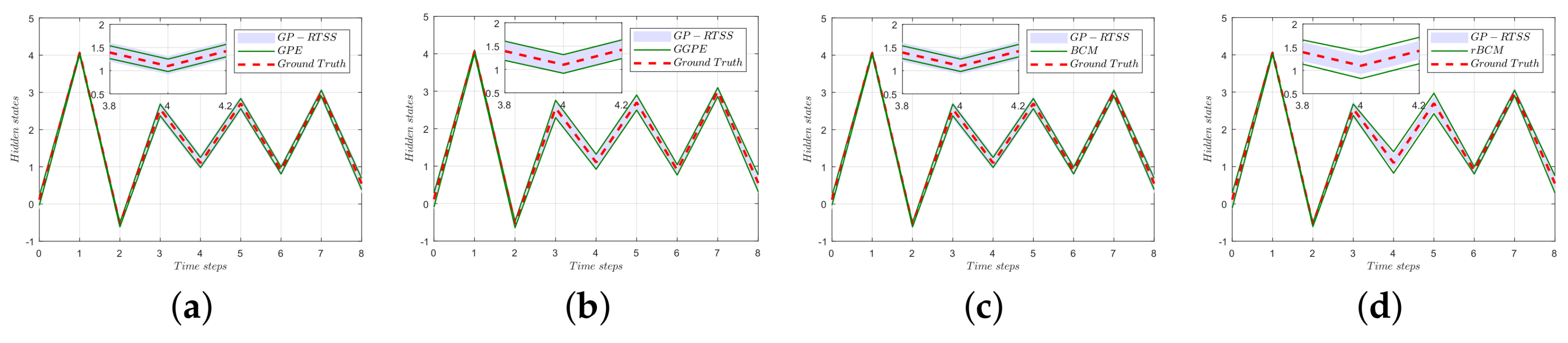
Moreover, we conduct an experiment with a one dimension problem [26]. Figure 4 shows the performance comparison of four distributed identification process (PoE , gPoE, BCM, rBCM) and robust Rauch-Tung-Striebel smoother for GP dynamic systems (GP-RTSS) [18], which is implemented under the full GP scheme. The PoE and BCM distributed schemes overestimate the variances in the regime of the series hidden states, which leads to overconfident precision compared with GP-RTSS. Moreover, the prediction of the rBCM is too conservative, although the rBCM aims to provide a more robust solution. The gPoE distributed scheme provides more reasonable identification of the hidden states than any other models in Figure 4.
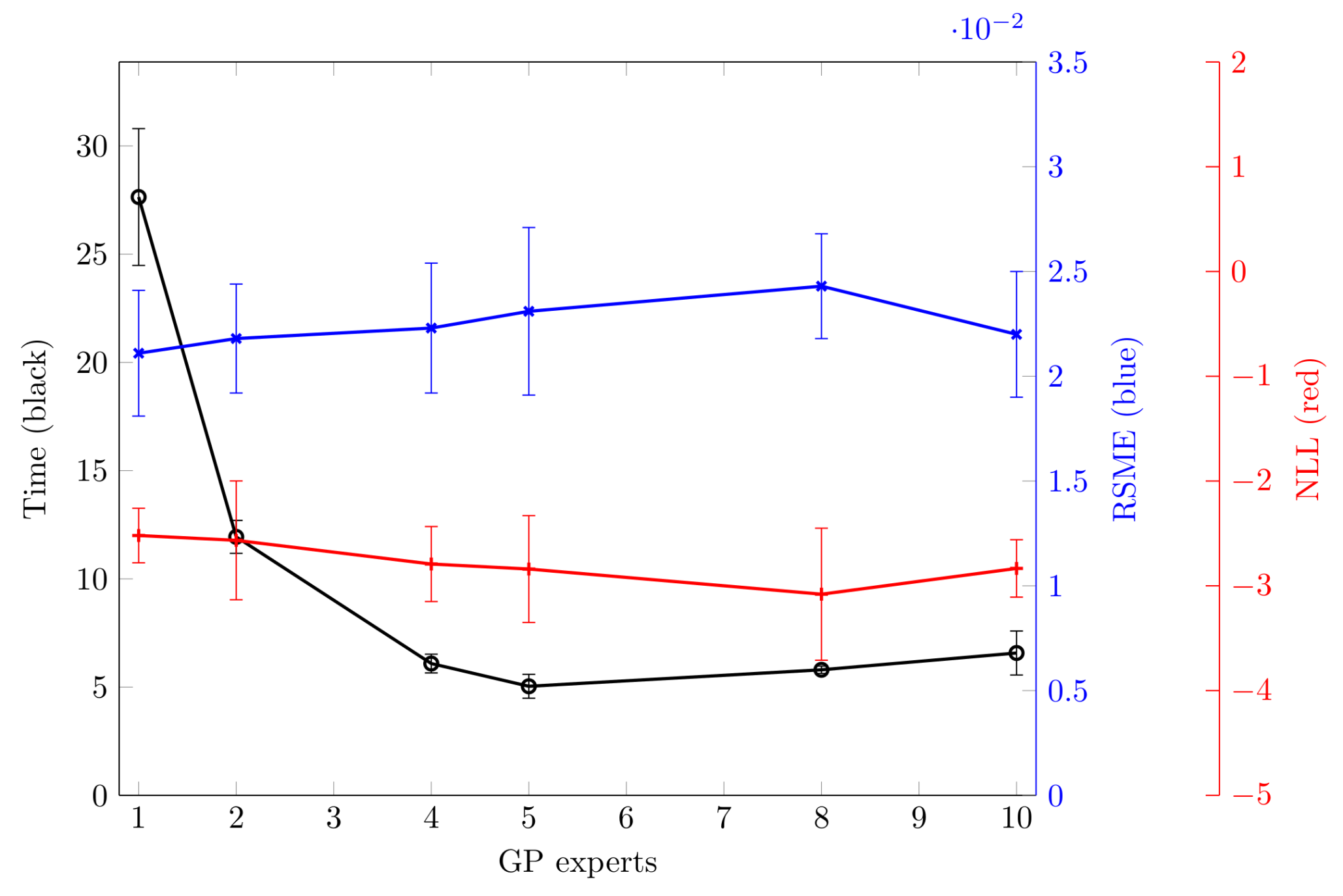
Moreover, Figure 5 shows two aspects of the distributed identification framework with the different number of GP experts: (1) a comparison of approximation quality; (2) computation expense. According to the information in Figure 5, for a certain set of training data, with the increase of the GP experts, the computation time significantly decreases. However, the computation expense reaches a minimum when there are five GP experts. Besides, the interesting properties are that there is no significant difference (root-mean-square-error (RSME): 0.01 and negative log-likelihood (NLL): 0.2) between the identification framework with one GP expert (full GP) and more than one expert. Furthermore, note that a better approximation quality can be expected with ten GP experts with the minima of RSME or with eight GP experts according to the NLL criterion. Thus, although we do not argue that our proposed hidden-state identification scheme outperforms the full GP identification algorithm concerning precision, the computation expense has been dramatically reduced. Moreover, the overall identification procedure is concluded in Algorithm 2.
| Algorithm 2: Inference with Monte Carlo Markov chain. |
 |
3. Evolving Learning of the Sensitivity Factor
The sensitivity amplification control proposed in [9] aims to improve the control performance without directly measuring the interaction information with the pilot. Thus, by inserting a sensitivity factor in dynamic equation:
The interaction between the pilot and the exoskeleton is given:
With perfect estimation and and sufficient large . The interaction d can approach zero. Nevertheless, the sensitivity factor should not be selected with a sufficiently large parameter due to the weak robustness. Moreover, in an actual situation, the interaction varies owing to stochastic environment factors. Therefore, choosing a fixed sensitivity factor is not a good option. An improvement has been made in [27], where the sensitivity factor is learned with Qlearning. Compared with the classic SAC, the interaction force has been reduced. However, the learning algorithm mainly copes with the discrete region of interest. In addition, the optimization of the constraint domain of the sensitivity factor is not addressed in the reference.
In this paper, the sensitivity factor is evolved in real time in a continuous constraint domain. By applying covariance matrix adaptation evolution strategy (-CMA-ES) [28], the sensitivity factor seeks the optimal value owing to tracking error penalty.
3.1. (1 + 1)-CMA-ES
Derived from the CMA-ES, a crucial feature of the -CMA-ES is that it directly operates on Cholesky decomposition and is about -times faster than the classic CMA-ES. The -CMA-ES adapts not only the entire covariance matrix of its offspring candidates, but also the entire step size. Since the covariance matrix is definitely positive, owing to Cholesky decomposition, , with an matrix. Thus, the offspring candidate is written:
where is the step size, is the corresponding parental candidate and is derived from normal distribution. In addition, the adaptation strategy maintains a search path in order to save an exponentially-fading record . Thus, a successful offspring candidate can be obtained from the covariance matrix:
With . Rather than dealing with the Cholesky decomposition operation in every loop, the matrix can be updated as follows:
With . To enhance the learning efficiency, if the offspring candidate solution is extremely unsuccessful, the algorithm should also learn from failure cases. Therefore, the covariance matrix update is written:
where ; similarly, the equivalent update of matrix is given:
The graphic interpretation of CMA-ES is shown in Figure 6. More specifically, the contributions of each sample are ranked according to corresponding penalties, which will be explained in the next subsection. Not all samples, but several high-contribution points are used during the update procedure. Thus, the new distribution is evolved from the previous step distribution with an adaptive step size.
3.2. Constraint Optimization
Since the sensitivity factor is constrained regarding the optimization domain, to deal with this problem, the variance of the offspring distribution is reduced in the normal vector direction in the vicinity of the corresponding parental candidate. For the constraints , an exponential fading vector is defined following [29] and updated when the optimization is lessened by the boundary:
where is a parameter that determines the convergence speed. Equation (20) can be seen as a low-pass filter, which guarantees that the tangential components of have been canceled out.
In these situations, the Cholesky factor should also be rewritten to meet the demand of the restrained boundary:
With and if , otherwise zero. The update size is controlled by the parameter . Moreover, compared with Equations (17) and (19), Cholesky decomposition A without a scalar greater than one aims to decrease the update step size to approach the boundary of constraints.
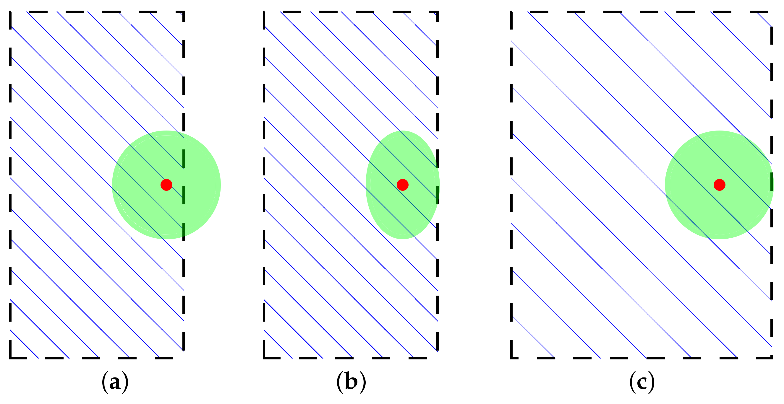
The solution to generating offspring candidates is explained in Figure 7. In the direction of the normal vector, the variance of the offspring is reduced as shown in Figure 7a. After the operation, the evolved variance is tangential to the constraint boundary in Figure 7b. Thus, the offspring candidates can be sampled and derived from the evolved variance . Note that, in Figure 7c, after constraint optimization, the constraint angle has been increased due to the change of the offspring distribution.
In terms of the sequence hidden-states , as well as actual data, the penalty function for updating of the sensitivity factor is given:
where and are the joint velocity and angle, separately. Note that not akin to the control algorithm in [27], where the penalty function consists of the previous loop trajectory data, the desired control input is computed and predicted from the identification process. Therefore, our scheme is more suitable for improving real-time control performance. The first term in Equation (22) is to avoid high jerk. Furthermore, the last two terms are penalized for tracking error. From our intuition, with less interaction force between the human and the exoskeleton, the pilot will feel more comfortable. According to this point view, punishing the last two terms may enhance the tracking performance. The main routine of the evolving learning of sensitivity factors scheme is presented in Algorithm 3.
| Algorithm 3: Evolving learning of the sensitivity factor. |
 |
4. Experiment and Discussion
Although the overall algorithm has been introduced in the previous part of this paper, the control performance of the algorithm should be verified. Consequently, in this section, first, we briefly explain our exoskeleton platform and distributed identification mode learning; then, we compare several state-of–the-art control methods (SAC, SAC + Qlearning) with our proposed control framework.
4.1. Experiment Setting and Model Learning
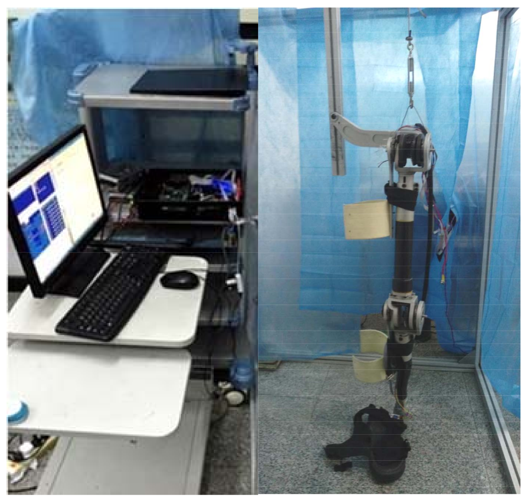
The developed single-leg exoskeleton platform is as shown in Figure 8, which is a robust and ergonomic device for endurance enhance and strength augmentation. The necessary auxiliary facilities are embedded industrial personal computer (IPC), PMAC (programmable multi-axis controller), Copley actuators and power supply unit. The power module should provide three kinds of voltage, i.e., 5 V, 12 V and 24 V. The observation data, derived from inertial measurement unit (IMU) and magnetic encoders, is collected by PMAC. The high-level control scheme is calculated in the embedded PC, and the driven commands are sent to the actuator through the Copley driver. For more details, we refer to our previous work in [30].
Before the implementation of the experiments, the dynamic and measurement models should be learned off-line. Therefore, to learning dynamic and measurement models, the necessary components are input, as well as observation. For dynamic models, the training input is given in a series of tuples () with and the next step state as training outputs. The input signal Nm is selected randomly and is constrained for safety. In addition, for measurement models, the training inputs are defined as system state given by the angles , and the corresponding angular velocities , , for hip joint and knee joint, respectively. To observe the system states, we apply the encoder and IMUs to measure the joint angles and angular velocities separately. Therefore, the training outputs of the measurement models are defined.
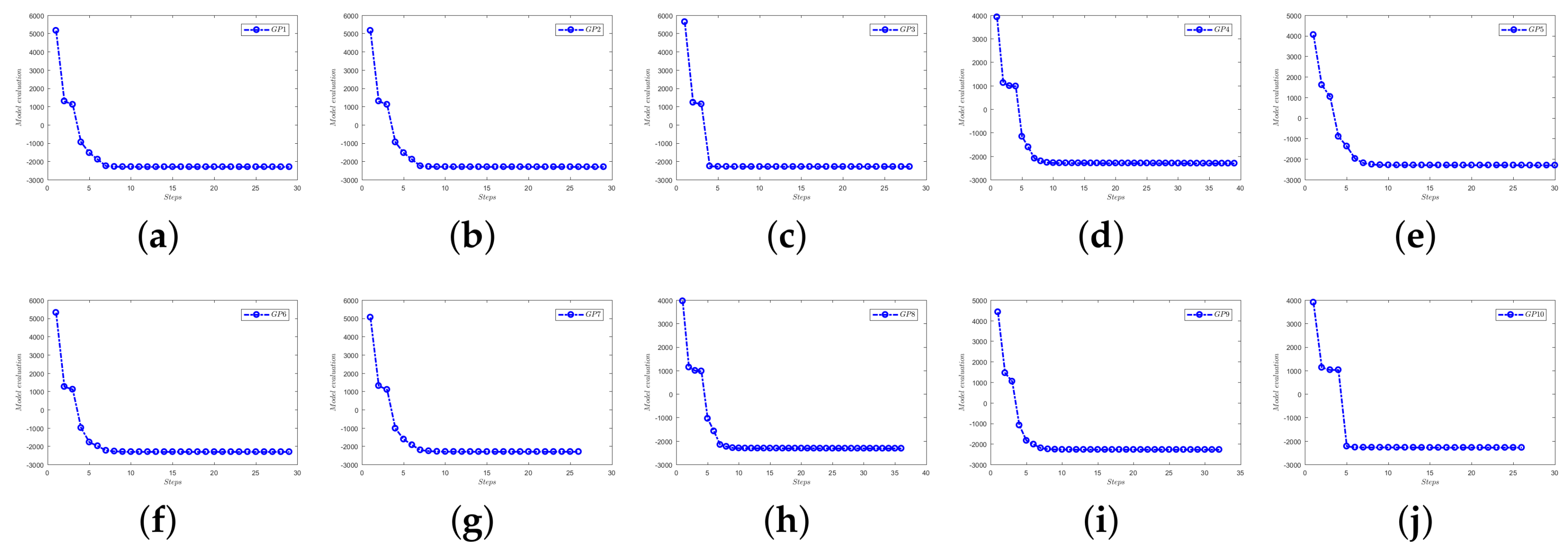
The learning result of the dynamic model of the hip joint is presented in Figure 9. Consequently, in order to learn the hyper-parameters each GP takes about 30–40 trails. Furthermore, the initial value of each function may be different owing to random initialization. Moreover, to demonstrate the feasibility, we test 600 unused data pairs with the learned model as shown in Figure 10. The error of the identification result compared with the system value is about 0.01 rad given in the lower figure of Figure 10.
4.2. Flat Walking Experiment
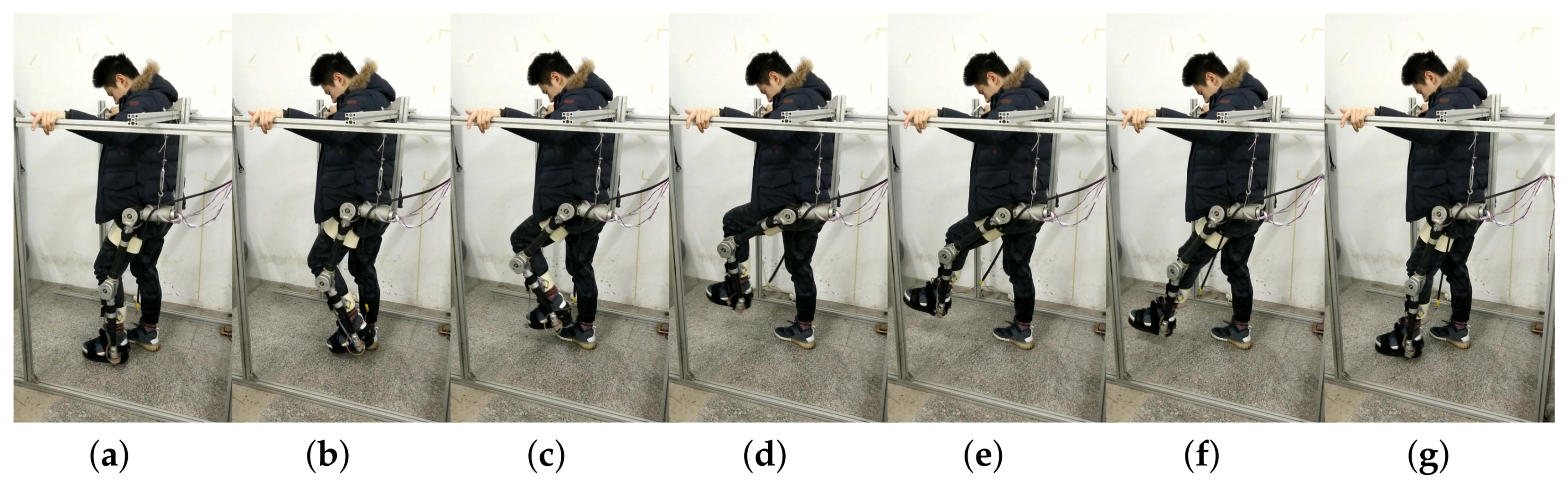
In the experiment, the pilot is asked to naturally swing his left leg, as shown in Figure 11. The control algorithms compared in the experiment are SAC [10], SAC + Qlearning [27], SAC + CMA-ES and our proposed algorithm.
The tracking performances of the knee joint and the hip joint are given in Figure 12a,b. Since the hidden states are identified, the single exoskeleton leg can follow the human motion in real time. Furthermore, owing to the CMA-ES algorithm, the evolution of the sensitivity factor for the hip joint is shown in Figure 12c, along with the evolution for the knee joint presented in Figure 12d. To be more specific, the updated distribution is derived from the contributions of 15 samples selected from 20 candidates. The lower bound and upper bound are set to be three and 10, respectively, according to experimental experience. Furthermore, from Figure 12c, the sensitivity factor of the hip joint increases as the pilot puts down his leg, which means that the HRI force decreases, and the exoskeleton does not need too much additional torque from the pilot. Consequently, setting a fixed sensitivity factor is not a good option. Moreover, compared with the hip-joint sensitivity factor, the knee-joint sensitivity factor almost keeps a lower one, fluctuating around four. The reason for this situation is that the interaction between the thigh and the exoskeleton is more compliant than the interaction between the shank and the exoskeleton. Therefore, the sensitivity of the hip joint is better than that of the knee joint.
In order to assess the control performance of our proposed algorithm, we compare the HRI force of four algorithms as shown in Figure 13. Since there is no sensor mounted between the pilot and exoskeleton, the HRI force is estimated by the disturbance observer. From intuition, the pilot feels more comfortable with less interaction force in the walking pattern. Therefore, the control performance may be evaluated from the information of the interaction force. As we all know, the ideal control performance is that the interaction force is zero, which means that the exoskeleton can follow the human motion perfectly.
Thus, to quantitatively evaluate the four control schemes, we compute the RMSE of the HRI of each joint. From Table 1, compared with the SAC control scheme, both SAC + Qlearning and SAC + CMA-ES own lower RMSE in both joints, since both algorithms learn an adaptive sensitivity factor. Furthermore, a small difference is shown in Table 1 between the SAC + Qlearning, as well as SAC + CMA-ES, and SAC + CMA-ES performs a little better. Moreover, a significant reduction of RMSE can be seen in Table 1 in our proposed algorithm, which is nearly two-times less than the other control schemes.
5. Conclusions
In this paper, a novel control framework has been proposed to address the crucial issues of SAC, i.e., weak robustness, disability to reject the disturbance and model uncertainties. The proposed control methodology, so-called probabilistic sensitivity amplification control, is two-fold: distributed hidden-state identification and evolving learning of sensitivity factors. The identification aims to enhance the robustness and to reject the undesired disturbance. The computation expense is significantly reduced owing to the distributed GP scheme. Moreover, the evolving learning is mainly designed to reduce the HRI between the pilot and the exoskeleton. Since the sensitivity factor can be evolved due to the punishment of the tracking error, the controller can learn from different HRI. Finally, several experiments have been implemented to verify the feasibility of our control scheme. The experimental result shows promising application feasibility. In our future work, we will extend our control scheme to a more complex situation, i.e., upper limb exoskeleton and whole body exoskeleton.
Acknowledgments
Part of this work has received funding from National Science Foundation of China under Grant No. 51521003. We gratefully acknowledge the constructive comments and suggestions of the reviewers.
Author Contributions
Likun Wang and Yi Shen conceived of and designed the experiments. Likun Wang, Wei Dong and Zhijiang Du performed the experiments. Likun Wang analyzed the data; Guangyu Zhao contributed experiment platform and devices. Likun Wang and Wei Dong wrote the paper.
Conflicts of Interest
The authors declare no conflict of interest.
References
- Kawamoto, H.; Sankai, Y. Power assist method based on phase sequence and muscle force condition for HAL. Adv. Robot. 2005, 19, 717–734. [Google Scholar] [CrossRef]
- Cruciger, O.; Schildhauer, T.A.; Meindl, R.C.; Tegenthoff, M.; Schwenkreis, P.; Citak, M.; Aach, M. Impact of locomotion training with a neurologic controlled hybrid assistive limb (HAL) exoskeleton on neuropathic pain and health related quality of life (HRQoL) in chronic SCI: a case study. Disabil. Rehabilit. Assist. Technol. 2016, 11, 529–534. [Google Scholar] [CrossRef] [PubMed]
- Sarasola-Sanz, A.; Irastorza-Landa, N.; López-Larraz, E.; Bibián, C.; Helmhold, F.; Broetz, D.; Birbaumer, N.; Ramos-Murguialday, A. A hybrid brain-machine interface based on EEG and EMG activity for the motor rehabilitation of stroke patients. In Proceedings of the 2017 IEEE International Conference on Rehabilitation Robotics (ICORR), London, UK, 17–20 July 2017; pp. 895–900. [Google Scholar]
- Fontana, M.; Vertechy, R.; Marcheschi, S.; Salsedo, F.; Bergamasco, M. The body extender: A full-body exoskeleton for the transport and handling of heavy loads. IEEE Robot. Autom. Mag. 2014, 21, 34–44. [Google Scholar] [CrossRef]
- Papini, G.R.; Avizzano, C.A. Transparent force control for Body Extender. In Proceedings of the 2012 IEEE RO-MAN, Paris, France, 9–13 September 2012; pp. 138–143. [Google Scholar]
- Anam, K.; Al-Jumaily, A.A. Active exoskeleton control systems: State of the art. Procedia Eng. 2012, 41, 988–994. [Google Scholar] [CrossRef]
- Kong, K.; Bae, J.; Tomizuka, M. Control of rotary series elastic actuator for ideal force-mode actuation in human–robot interaction applications. IEEE/ASME Trans. Mech. 2009, 14, 105–118. [Google Scholar] [CrossRef]
- Kim, S.; Bae, J. Force-mode control of rotary series elastic actuators in a lower extremity exoskeleton using model-inverse time delay control (MiTDC). IEEE/ASME Trans. Mech. 2017, 22, 1392–1400. [Google Scholar] [CrossRef]
- Kazerooni, H.; Racine, J.L.; Huang, L.; Steger, R. On the control of the berkeley lower extremity exoskeleton (BLEEX). In Proceedings of the 2005 IEEE International Conference on Robotics and Automation (ICRA), Barcelona, Spain, 18–22 April 2005; pp. 4353–4360. [Google Scholar]
- Kazerooni, H.; Steger, R.; Huang, L. Hybrid control of the Berkeley lower extremity exoskeleton (BLEEX). Int. J. Robot. Res. 2006, 25, 561–573. [Google Scholar] [CrossRef]
- Kong, K.; Bae, J.; Tomizuka, M. A compact rotary series elastic actuator for human assistive systems. IEEE/ASME Trans. Mech. 2012, 17, 288–297. [Google Scholar] [CrossRef]
- Wang, L.; Du, Z.; Dong, W.; Shen, Y.; Zhao, G. Intrinsic Sensing and Evolving Internal Model Control of Compact Elastic Module for a Lower Extremity Exoskeleton. Sensors 2018, 18, 909. [Google Scholar] [CrossRef] [PubMed]
- Sankai, Y. HAL: Hybrid assistive limb based on cybernics. In Robotics Research; Springer: London, UK, 2010; pp. 25–34. [Google Scholar]
- Suzuki, K.; Mito, G.; Kawamoto, H.; Hasegawa, Y.; Sankai, Y. Intention-based walking support for paraplegia patients with Robot Suit HAL. Adv. Robot. 2007, 21, 1441–1469. [Google Scholar]
- Ghan, J.; Kazerooni, H. System identification for the Berkeley lower extremity exoskeleton (BLEEX). In Proceedings of the 2006 IEEE International Conference on Robotics and Automation (ICRA), Orlando, FL, USA, 15–19 May 2006; pp. 3477–3484. [Google Scholar]
- Ko, J.; Fox, D. GP-BayesFilters: Bayesian filtering using Gaussian process prediction and observation models. Auton. Robots 2009, 27, 75–90. [Google Scholar] [CrossRef]
- Deisenroth, M.P.; Huber, M.F.; Hanebeck, U.D. Analytic moment-based Gaussian process filtering. In Proceedings of the 26th Annual International Conference on Machine Learning, Montreal, QC, Canada, 14–18 June 2009; pp. 225–232. [Google Scholar]
- Deisenroth, M.P.; Turner, R.D.; Huber, M.F.; Hanebeck, U.D.; Rasmussen, C.E. Robust filtering and smoothing with Gaussian processes. IEEE Trans. Autom. Control 2012, 57, 1865–1871. [Google Scholar] [CrossRef] [Green Version]
- Eleftheriadis, S.; Nicholson, T.F.; Deisenroth, M.P.; Hensman, J. Identification of Gaussian Process State Space Models. arXiv, 2017; arXiv:1705.10888. [Google Scholar]
- Deisenroth, M.P.; Ng, J.W. Distributed gaussian processes. arXiv, 2015; arXiv:1502.02843. [Google Scholar]
- Rasmussen, C.E. Gaussian processes in machine learning. In Advanced Lectures on Machine Learning; Springer: Berlin, Germany, 2004; pp. 63–71. [Google Scholar]
- Turner, R.; Deisenroth, M.; Rasmussen, C. State-space inference and learning with Gaussian processes. In Proceedings of the Thirteenth International Conference on Artificial Intelligence and Statistics, Sardinia, Italy, 13–15 May 2010; pp. 868–875. [Google Scholar]
- Ng, J.W.; Deisenroth, M.P. Hierarchical mixture-of-experts model for large-scale Gaussian process regression. arXiv, 2014; arXiv:1412.3078. [Google Scholar]
- Cao, Y.; Fleet, D.J. Generalized product of experts for automatic and principled fusion of Gaussian process predictions. arXiv, 2014; arXiv:1410.7827. [Google Scholar]
- Tresp, V. A Bayesian committee machine. Neural Comput. 2000, 12, 2719–2741. [Google Scholar] [CrossRef] [PubMed]
- Kitagawa, G. Monte Carlo filter and smoother for non-Gaussian nonlinear state space models. J. Comput. Graph. Stat. 1996, 5, 1–25. [Google Scholar]
- Huang, R.; Cheng, H.; Guo, H.; Chen, Q.; Lin, X. Hierarchical interactive learning for a human-powered augmentation lower exoskeleton. In Proceedings of the 2016 IEEE International Conference on Robotics and Automation (ICRA), Stockholm, Sweden, 16–21 May 2016; pp. 257–263. [Google Scholar]
- Arnold, D.V.; Hansen, N. Active covariance matrix adaptation for the (1 + 1)-CMA-ES. In Proceedings of the 12th Annual Conference on Genetic and Evolutionary Computation, Portland, OR, USA, 7–11 July 2010; pp. 385–392. [Google Scholar]
- Arnold, D.V.; Hansen, N. A (1 + 1)-CMA-ES for constrained optimization. In Proceedings of the 14th Annual Conference on Genetic and Evolutionary Computation, Philadelphia, PA, USA, 7–11 July 2012; pp. 297–304. [Google Scholar]
- Long, Y.; Du, Z.; Cong, L.; Wang, W.; Zhang, Z.; Dong, W. Active disturbance rejection control based human gait tracking for lower extremity rehabilitation exoskeleton. ISA Trans. 2017, 67, 389–397. [Google Scholar] [CrossRef] [PubMed]
Figure 1.
Proposed control framework. In the feedforward control loop, the sensitivity amplification control (SAC) controller with the evolving sensitivity factor (in black dashed arrow) provides the necessary driven torque according to the variational HRI (human-robot interaction, given in double blue arrows). Moreover, to improve the control performance, the hidden-states are identified in the feedback control loop according to the observation information. Note that, the red color arrows stand for input and output, while the black arrows present the signal direction.
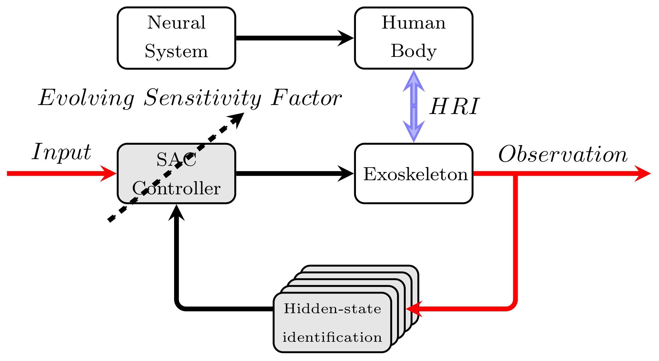
Figure 2.
Graphic explanation of the Gaussian process (GP) state-space inference and distributed hidden-state identification. Derived from the distributed GP framework, the hidden state variables (embedded in the gray circles) are identified by the dynamic models and the measurement models , separately. Also, the connection is presented in the red arrows and the influence of the input to the control plant is shown in the blue arrows. Note that the hyper-parameters related to the dynamic models are shared in the training process (in green arrows), along with the hyper-parameters for measurement models. (a) GP state-space inference; (b) proposed distributed hidden-state identification.

Figure 3.
The graphic interpretation of the Monte Carlo sampling. The real distribution in the dashed blue line is not the GP type, but approximated as GP in the solid blue line with the mean and covariance of the corresponding data.
Figure 3.
The graphic interpretation of the Monte Carlo sampling. The real distribution in the dashed blue line is not the GP type, but approximated as GP in the solid blue line with the mean and covariance of the corresponding data.
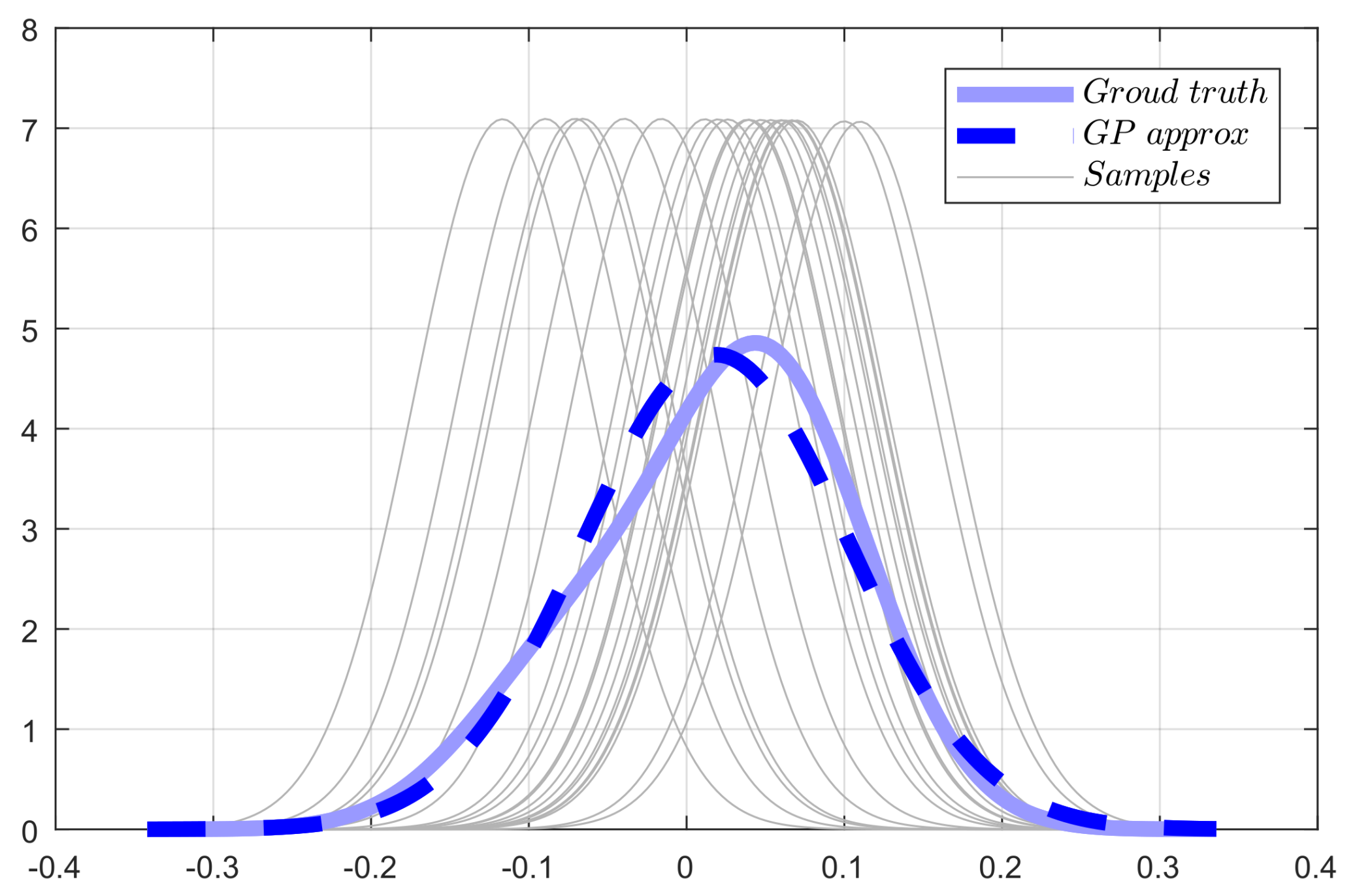
Figure 4.
Comparison of four data fusion methods for distributed hidden-state identification. In each subfigure, the confidence interval of the comparison algorithm is filled between two green lines. Furthermore, the GP-RTSS (full GP) to be approximated is shown in the blue shaded area, representing of the confidence interval, and the ground truth is given in the red dashed line. (a) PoE; (b) gPoE ; (c) BCM; (d) rBCM.

Figure 5.
Computation time, RSME and NLL for the different number of GP experts. The computation time is measured in MATLAB 2015b (MathWorks Company, USA) on a laptop ( 2.6 GHz cores and 8 GB RAM) with a Ubuntu 16.04 system (Canonical Ltd., UK). Each case of different numbers of GP experts is tested 20 times for the purpose of reducing the stochastic data influence.

Figure 6.
Visualization of CMA-ES exploration and updating rules. In (a), the new distribution is shown in the red ellipse, while the last-step distribution is in blue. The quantity of the contributions of each sample is defined with the area of the green circles. Consequently, these contributions are also ranked in (b). (a) Sampling, estimation and new distribution; (b) contributions of the samples.
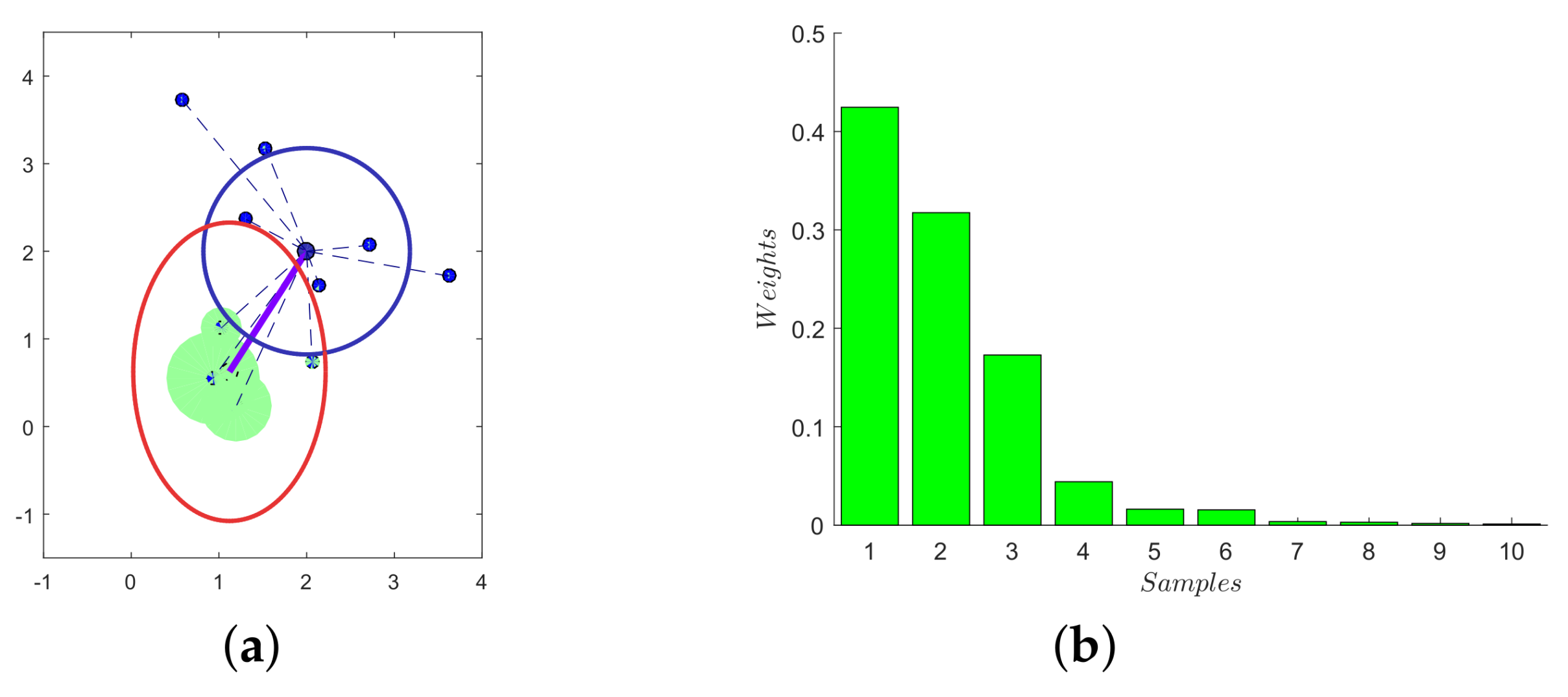
Figure 7.
Evolved variance of the offspring distribution along the normal direction of the boundary. (a) Original distribution; (b) reduced distribution; (c) inverse Cholesky decomposition. Additionally, the parent is donated as red point, while the offspring distribution is given in green circle (ecllipse). The gradient direction is define with blue dashed line.

Figure 8.
Exoskeleton robotic platform. The safety concern for our pilot is from two aspects, i.e., hardware precaution, as well as programming. Accordingly, exceeding of the motion is prohibited by the mechanical limit, and the system will be shut down if an error occurs.
Figure 8.
Exoskeleton robotic platform. The safety concern for our pilot is from two aspects, i.e., hardware precaution, as well as programming. Accordingly, exceeding of the motion is prohibited by the mechanical limit, and the system will be shut down if an error occurs.

Figure 9.
Evaluation of m GPs (). According to the distributed framework, the ten GPs share the same hyper-parameters. (a) GP1; (b) GP2; (c) GP3; (d) GP4; (e) GP5; (f) GP6; (g) GP7; (h) GP8; (i) GP9; (j) GP10.
Figure 9.
Evaluation of m GPs (). According to the distributed framework, the ten GPs share the same hyper-parameters. (a) GP1; (b) GP2; (c) GP3; (d) GP4; (e) GP5; (f) GP6; (g) GP7; (h) GP8; (i) GP9; (j) GP10.

Figure 10.
Cross-validation of the learned identification model. For the purpose of verifying the learning result of the identification model, we conduct a cross-validation with 600 successive data pairs. The state-space inferences of the hip joint, ground truth and the prediction error are presented in the above figure.

Figure 11.
Flat walking experiment. (a) Initial ground contact; (b) heel rise; (c) initial swing; (d) middle swing; (e) terminal swing; (f) heel strike; (g) full ground contact. The interaction between the pilot and the exoskeleton is made possible with the compliant cuff. Moreover, the pilot is asked to naturally sway his left leg.

Figure 12.
Tracking performances and evolution of sensitivity factors. (a) Tracking performance of the hip joint; (b) tracking performance of the knee joint; (c) evolution sensitivity factor of the hip joint; (d) evolution sensitivity factor of the knee joint.
Figure 12.
Tracking performances and evolution of sensitivity factors. (a) Tracking performance of the hip joint; (b) tracking performance of the knee joint; (c) evolution sensitivity factor of the hip joint; (d) evolution sensitivity factor of the knee joint.
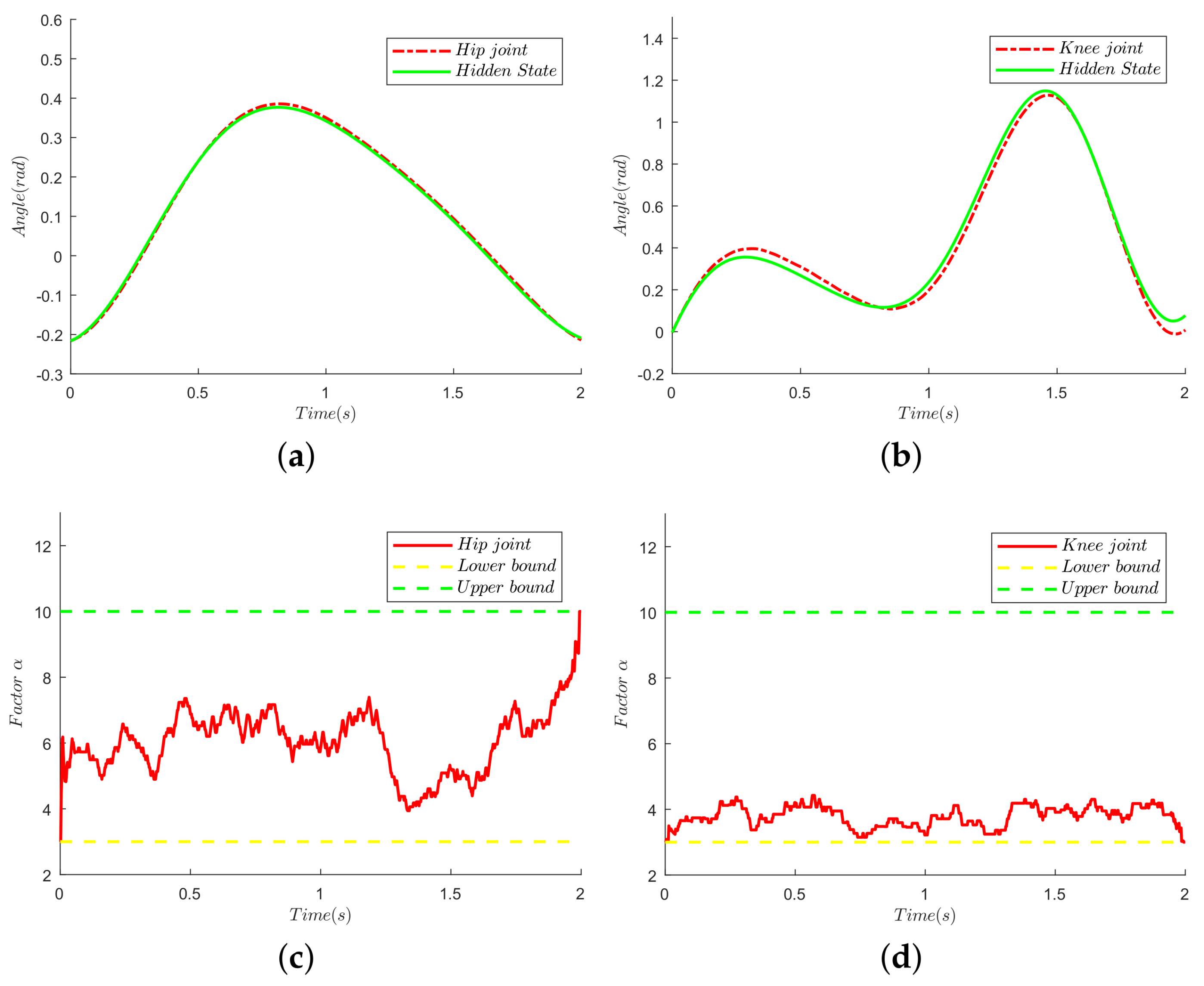
Figure 13.
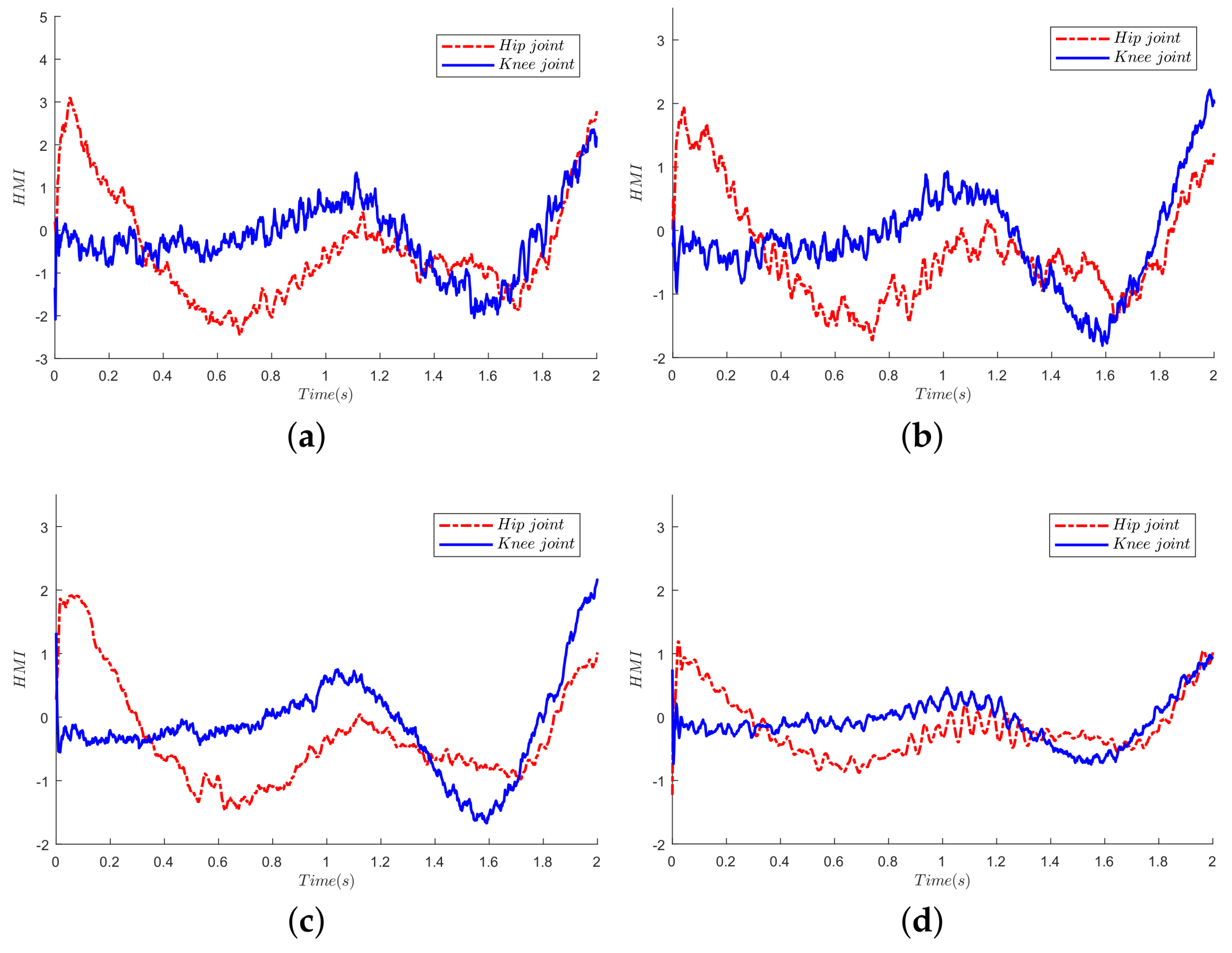
The HRI comparison of four control algorithms. (a) SAC; (b) SAC + Qlearning; (c) SAC + CMA-ES; (d) proposed algorithm. Note that the HRI force is estimated by the disturbance observer since there is no sensor mounted between the human and exoskeleton.
Figure 13.
The HRI comparison of four control algorithms. (a) SAC; (b) SAC + Qlearning; (c) SAC + CMA-ES; (d) proposed algorithm. Note that the HRI force is estimated by the disturbance observer since there is no sensor mounted between the human and exoskeleton.

© 2018 by the authors. Licensee MDPI, Basel, Switzerland. This article is an open access article distributed under the terms and conditions of the Creative Commons Attribution (CC BY) license (http://creativecommons.org/licenses/by/4.0/).
Share and Cite
MDPI and ACS Style
Wang, L.; Du, Z.; Dong, W.; Shen, Y.; Zhao, G. Probabilistic Sensitivity Amplification Control for Lower Extremity Exoskeleton. Appl. Sci. 2018, 8, 525. https://doi.org/10.3390/app8040525
AMA Style
Wang L, Du Z, Dong W, Shen Y, Zhao G. Probabilistic Sensitivity Amplification Control for Lower Extremity Exoskeleton. Applied Sciences. 2018; 8(4):525. https://doi.org/10.3390/app8040525
Chicago/Turabian StyleWang, Likun, Zhijiang Du, Wei Dong, Yi Shen, and Guangyu Zhao. 2018. "Probabilistic Sensitivity Amplification Control for Lower Extremity Exoskeleton" Applied Sciences 8, no. 4: 525. https://doi.org/10.3390/app8040525
Note that from the first issue of 2016, this journal uses article numbers instead of page numbers. See further details here.