1. Introduction
Convolutional auto-encoder (CAE), a kind of convolutional neural network (CNN), adopts an unsupervised learning algorithm for encoding [
1,
2,
3,
4,
5]. David E. Rumelhart first proposed the concept of an auto-encoder [
6] and employed it to process data with large dimensions, which promoted the development of neural networks. In 2006, Hinton et al. [
7] improved the original shallow auto-encoder and proposed the concept of a deep learning neural network as well as its training strategy, which can be used in the signal processing field for applications such as feature extraction [
8], image compression [
9,
10,
11], classification [
12,
13], image denoising [
14], prediction [
15], and so on. Wang et al. [
16] proposed a rapid 3D feature learning method named a convolutional auto-encoder extreme learning machine (CAE-ELM), and the features extracted were superior to other previous deep learning methods. In [
17], a three-layer multilayer perceptron structure was presented for image compression, which verified the applicability of the neural network in the field of image compression. Kim et al. [
18] performed sonar image noise reduction with the CAE and obtained sonar images of superior quality with only a single continuous image. However, there is the same problem that the above applications running on CPU are all inefficient and time-consuming. To address this problem, GPU has been employed to accelerate the neural network [
19,
20], but the power consumption of GPU is too large.
A field programmable gate array (FPGA) breaks through the sequential execution mode of general-purpose processors, and is able to implement a neural network with high speed. In [
21,
22], two deep convolutional neural network (DCNN) accelerators were proposed which optimized the energy efficiency of the system by reducing the complexity of data transmission. Zhou et al. [
23] used a fixed-point data type to represent parameters for computation based on FPGA, which achieved better performance and lower resource usage. To further enhance the performance, some researchers exploited the inherent parallelism of neural networks and utilized the multi-hardware and multi-product unit on FPGA to realize the network framework [
24,
25]. From the above references [
21,
22,
23,
24,
25], we conclude that it is promising to accelerate neural networks by employing FPGA, which can make full use of the parallel processing characteristic of FPGA and the parallel computing framework of the neural network. However, the finite resource of FPGA makes it difficult to realize a neural network on a large scale.
To enhance the processing speed and reduce the power consumption and resource occupation, we propose a novel CAE using a periodic layer-multiplexing method, which periodically reuses only one layer to establish the network. On the one hand, by fixing the number of channels, this framework can be applicable to images of arbitrary size. On the other hand, to effectively improve the speed of convolution calculation, the parallel convolution method is used based on shift registers. The image compression is taken as an example to evaluate the performance of the proposed CAE framework. Experimental results show that our framework has advantages in terms of resource occupation, operational speed, and power consumption.
The rest of the paper is arranged as follows. In
Section 2, the CAE framework and its key techniques are described in detail. In
Section 3, experimental results and discussion are given. Finally, some conclusions are drawn in
Section 4.
2. FPGA Implementation of the CAE
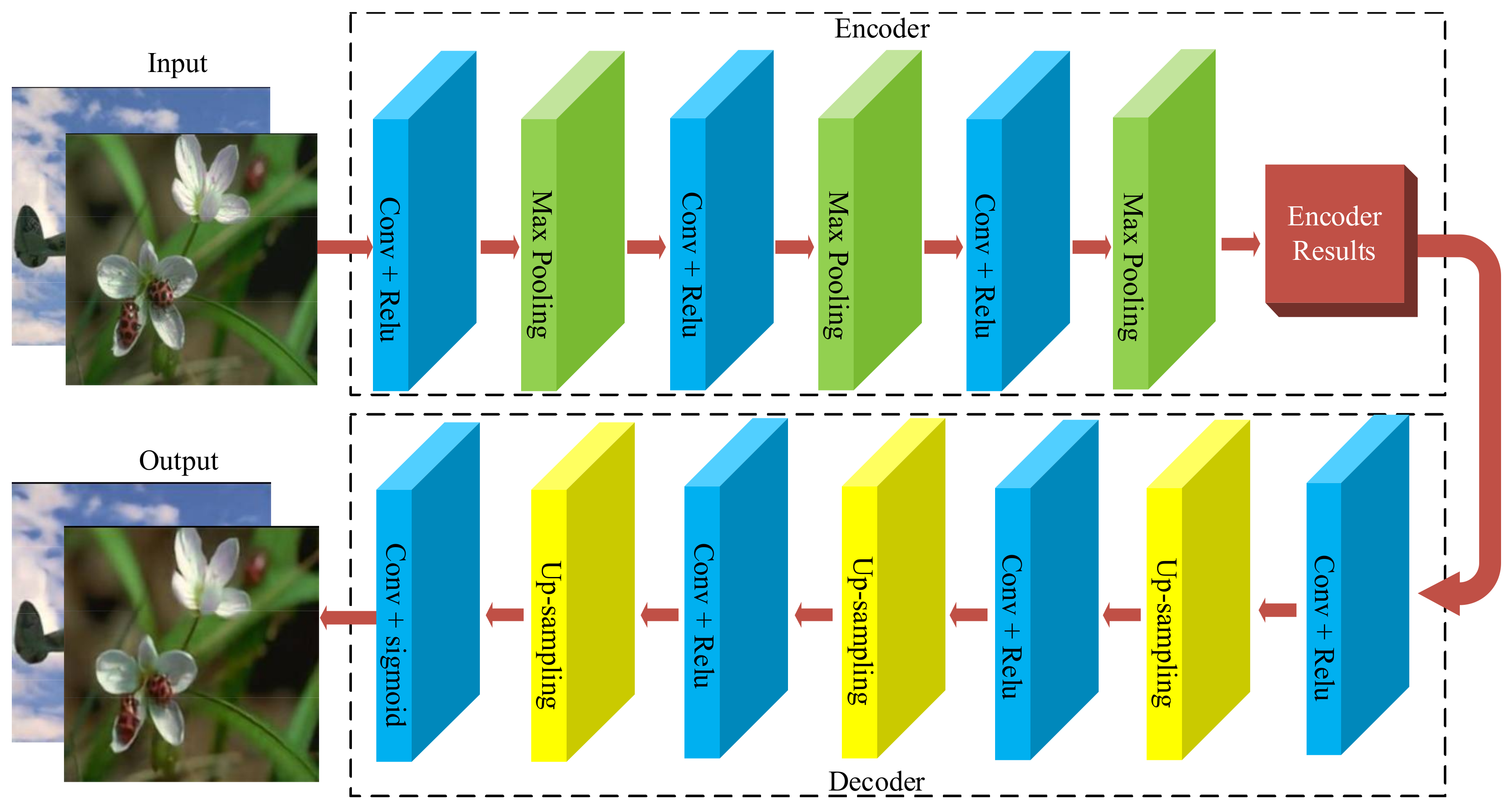
In essence, CAE is a multilayer CNN including convolution layers and pooling layers. The model of CAE used is shown in
Figure 1, where the image compression is taken as an example. The convolution layers are mainly used to extract the features of inputs and the neurons in these layers share the weight parameters. The pooling layers are used to retain the main features and reduce the parameters, which also prevent overfitting and improve the generalization ability of the model. The upsampling process is performed to obtain the image in original resolution, which can be considered the inverse process of pooling.
The model is divided into two parts: an encoder and a decoder. The encoder contains three convolutional layers and three pooling layers. The ReLU function and the maximum pooling operation are used. The decoder, which performs the reverse operation of the encoder, consists of four convolution layers and three upsampling layers. The ReLU function and the sigmoid function are used in the first three and the last convolution layers, respectively.
From
Figure 1, it can be seen that the layers of CAE have a certain regularity and periodicity, so we implement their functions by proposing the periodic layer-multiplexing framework based on FPGA. The hardware framework and the relative key techniques are described as follows.
2.1. Hardware Framework
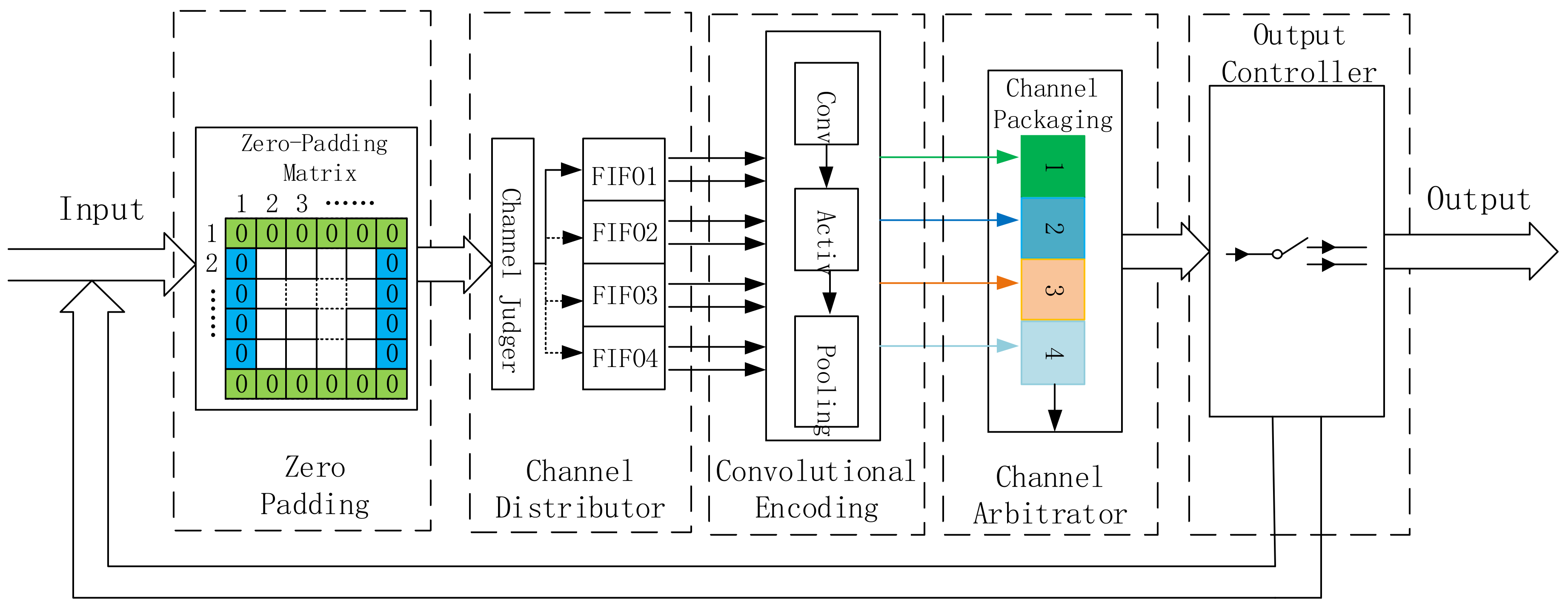
As shown in
Figure 2, the encoder part of the proposed CAE framework contains five main modules: zero padding, a channel distributor, convolutional encoding, a channel arbitrator, and an output controller. The detailed explanation is as follows:
(1) Zero Padding Module
To prevent losing the boundary information during the convolution operation, the zero padding module is employed to fill zeros around the input matrix. The obtained matrix is defined as the zero-padding matrix in this paper.
(2) Channel Distributor Module
The zero-padding matrix is sent to the channel distributor module, which contains a channel judger and four first-in, first-out (FIFO) memories. The channel judger interleaves every two single-channel data points and then sends them to the FIFOs in sequence. The FIFOs buffer the interleaved data, and then divide them into eight channels.
(3) Convolutional Encoding Module
The work process of this module is summarized as follows: First, the convolution layers in this module execute the convolution calculation in eight channels at the same time. The convolution kernels, obtained by training CAE, are stored directly in the internal LUT resources. By this means, the frequent data interaction between FPGA and external memory is avoided, and the transmission latency is reduced significantly. Then, in order to introduce nonlinear factors after the convolution calculation, activation functions are integrated into the convolution layers. Specifically, the ReLU function is employed for fast convergence and high accuracy. Finally, the maximum pooling is chosen to retain the main features. The first set of eight-channel data is transformed to the three-channel data after the pooling operation, while the subsequent sets of eight-channel data are transformed to the four-channel data.
(4) Channel Arbiter Module
The output data of the convolutional encoding module are orderly packaged as the single-channel data, and then sent to the next module by the channel arbiter module for judgment.
(5) Output Controller Module
This module is used to judge whether the data stream is processed completely. The above modules process continuously until the ending data of the zero-padding matrix are handled.
2.2. Design of Convolutional Encoding Module
Convolutional encoding is the most important module in the framework; therefore, its structure is further discussed below. To effectively enhance the compatibility of our framework and control the utilization of hardware resources reasonably, the number of input channels is fixed to eight rather than the maximum number of neurons in a certain layer. To realize the simultaneous convolution calculation of eight channels, the parallel channels method is developed by caching the input data.
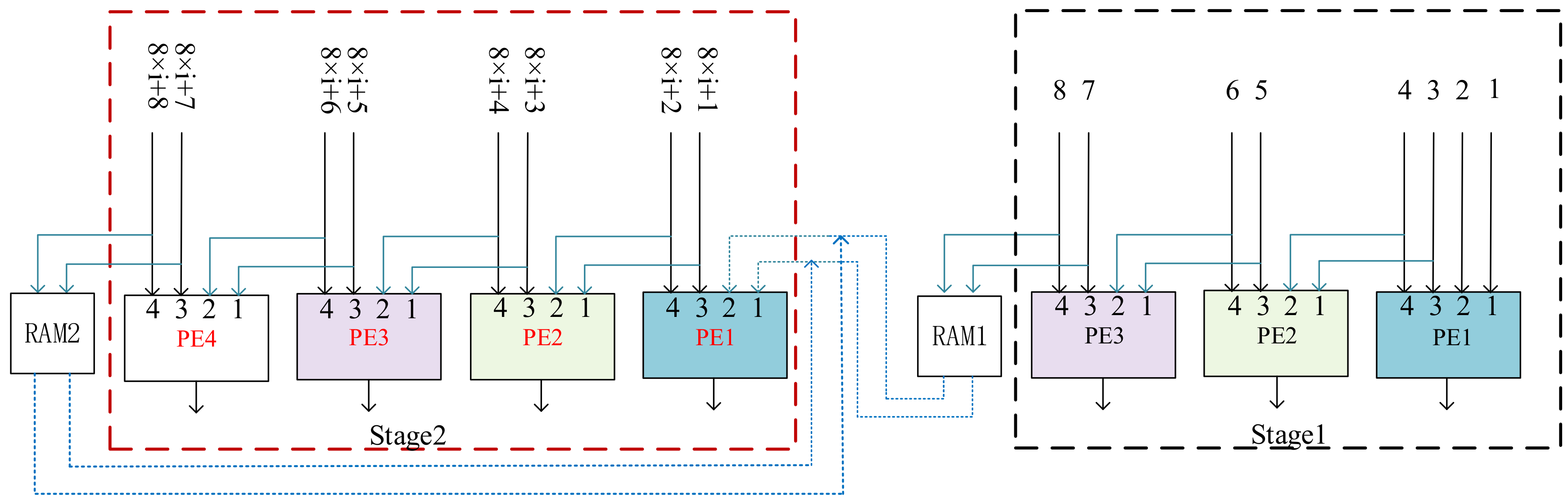
The operational process of the method is shown in
Figure 3. Four identical processing elements (PEs) are used to process the input data, and the ones with identical sequence number are the same. These PEs are independent of each other so they can operate simultaneously. Therefore, all the convolutional results of the eight channels can be calculated simultaneously by inputting the data in sequence. The RAM1 and RAM2 are used to cache the last two-channel data of every eight inputs, which can avoid loading repetition of the input and improve the efficiency of data utilization. In
Figure 3, 8 ×
i +
j (
i = 1,…, ⌈M/8⌉ − 1 and
j = 1,2,...,8) represents the index of channel. Meanwhile, M represents the total number of rows of zero-padding matrix, and the symbol ⌈⌉ represents a rounding-up operation.
At stage 1 (the black box in
Figure 3), the first two inputs are transmitted to the first two channels of PE1, while the next two inputs are transmitted simultaneously to the other channels of PE1 and the first two channels of PE2. The next two inputs are provided to both the last two channels of PE2 and the first two channels of PE3. The last two inputs are sent to the last two channels of PE3 and RAM1 at the same time. The RAM1 is employed to buffer data, so that these data can be recycled without re-entering from outside. As shown in
Figure 3, once the first set of eight-channel data from the zero-padding matrix has been processed at stage 1, the subsequent set of eight-channel data is sent to PEs at stage 2 (red box in
Figure 3). At stage 2, the data in RAM1 and the subsequent inputs are sent to PEs, and a similar operation is undertaken as that at stage 1.
2.3. Design of PE
The PEs employed by the periodic layer-multiplexing framework are used to implement the operation of multiplication and addition required by convolution calculation. To reduce the time consumption of convolution calculation, a parallel convolution method based on shift registers is presented for the design of PE.
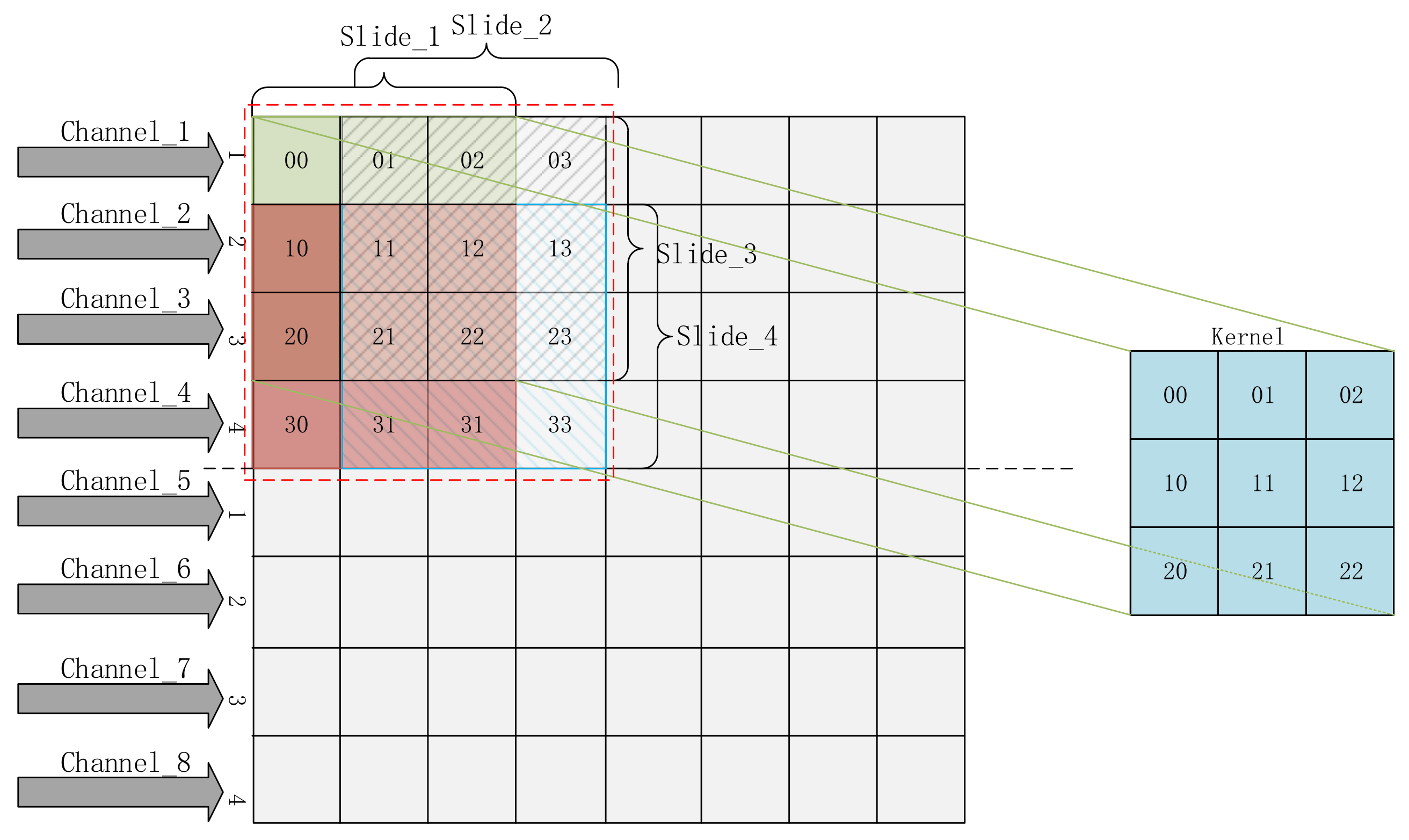
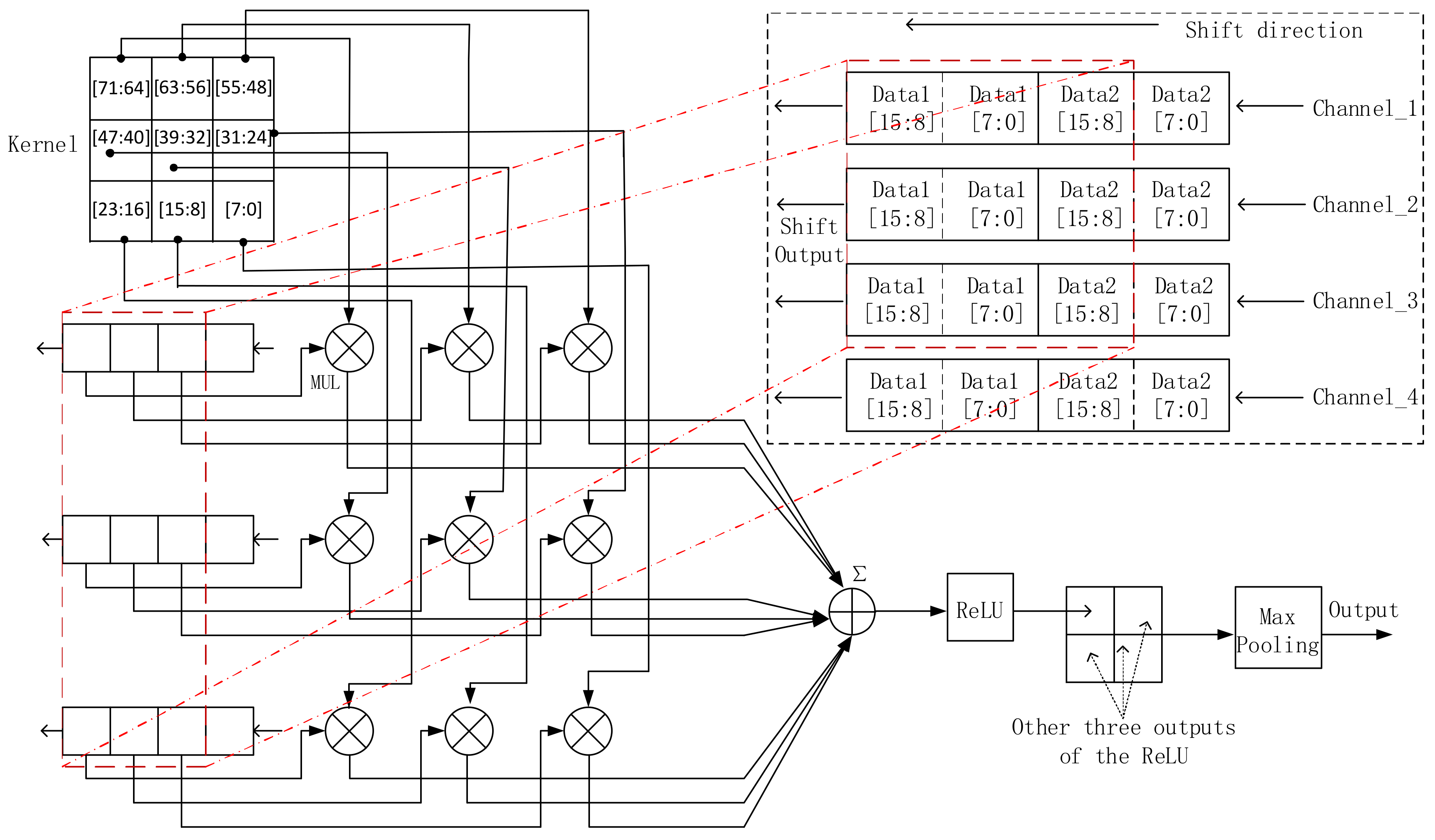
There are four input channels in one PE, and the 16-bit unsigned numbers in the four channels can be inputted to the corresponding 32-bit shift registers per clock cycle. These 32-bit shift registers act as the convolution window, which can slide arbitrarily. We first assume that the data are inputted to these shift registers immediately after reset. Then, the convolution calculations begin in the second clock cycle. A 4 × 4 convolution window of the PE is shown as the colorful square in
Figure 4.
For storage convenience, a total of nine 8-bit signed numbers of each convolution kernel are combined in a row to form an integrated data with a width of 72 bits. When the convolution calculation starts, the convolution window begin to slide so that convolution operations can be performed in the four sub-windows simultaneously under one clock cycle. Then every 8-bit convolution kernel is multiplied by the data in the shift register, as shown in
Figure 5. After that, the outputs of multipliers are obtained under the third clock cycle. All these outputs of multipliers are summed and exported under the fourth clock cycle. Some nonlinear factors are introduced into these results by operating the ReLU activation function. The outputs of all the ReLU functions are transmitted to the pooling module, and then three comparators in this module start to perform comparison operation among the four values and output the maximum, which consumes two clock cycles.
The pseudo-code of the operation is as follows (algorithm 1):
| Algorithm 1. The algorithm of convolution operation process in PE. |
Initialization: Reset the system and cache the parameters.
Input: The eight channels image data: data_in, are inputted.
Shift: data_shift [31:0] = {data_shift [15:0], data_in};
Convolution: for(row = 0, row ≤ 1, row++){
for(col = 0, col ≤ 1, col ++){
for(p = 0, p ≤ 2, p++) {
for(q = 0, q ≤ 2, q++){
data_convolution [row][col]+ = kernel[p] [q] × data_shift [row + p] [col + q];}}}
Activation: Execute the ReLU function.
Pooling: Compare and then give the max value. (0 ≤ {row,col} ≤ 1)
Return: Output the pooling result. |
3. Experimental Results and Discussion
In order to test the performance of the proposed implementation of CAE, an application of image compression is carried out. We use Keras, which is a Python deep learning library, to establish the framework. There are 7000 digital images with a dimension of 256 × 256 × 3 employed to train the network and obtain the parameters. During training, the epoch of iteration is chosen to be 1500, while the batch size is chosen to be 4. The binary_crossentropy cost function, which can avoid the training process being too slow, is selected as the loss function. It has a non-negative character and when the real output is close to the expected output, the function value is close to 0. The learning rate is chosen to be Adadelta, which is an adaptive learning rate method. The test starts once the training is finished. In this paper, 1000 additional images are employed to verify the performance of image compression based on the proposed CAE.
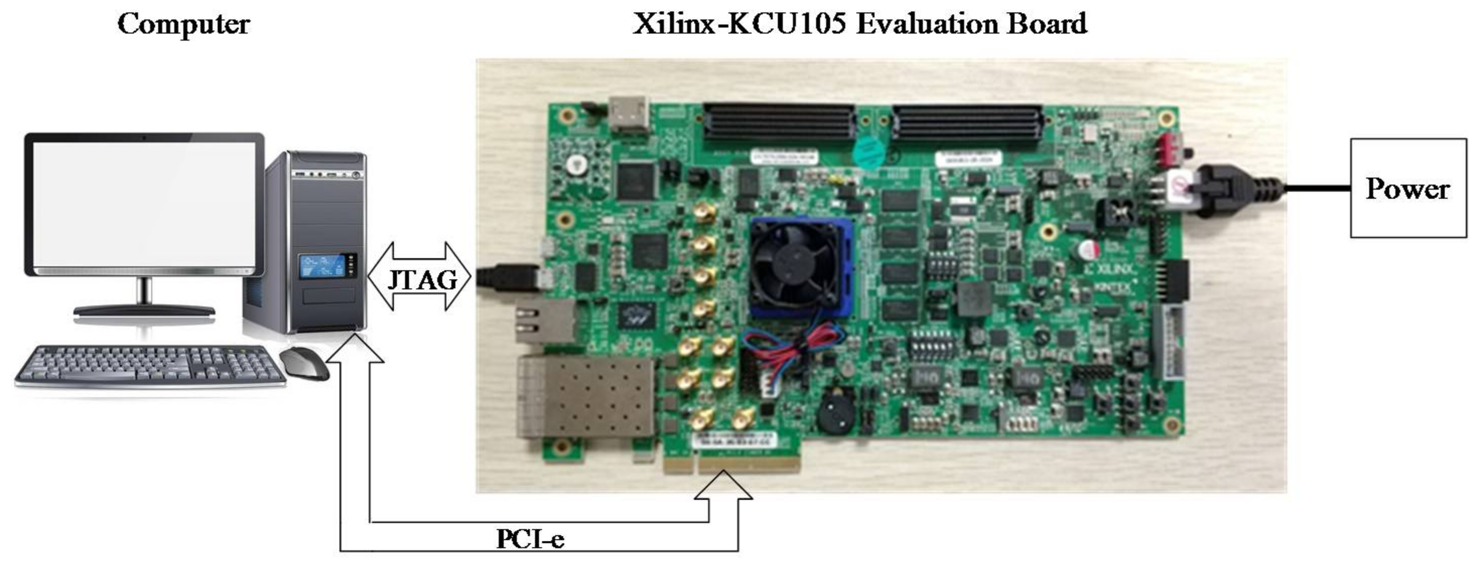
In this experiment, the Xilinx KCU105 evaluation board (Xilinx, San Jose, CA, USA) with a XCKU040-2FFVA1156E FPGA chip (Xilinx, San Jose, CA, USA) is employed to act as the hardware platform. The photograph of the implemented prototype is shown in
Figure 6, from which we can see that the evaluation board is connected to a computer by JTAG cable and PCI-e bus. FPGA is programmed and debugged through the JTAG cable, while the data are transferred between the computer and FPGA through the PCI-e bus.
In order to measure the performance of our compression framework, we can use some typical metrics, such as compression ratio, Peak Signal to Noise Ratio (PSNR), and Multi-scale structural similarity (MS-SSIM). The image compression ratio obtained from a CAE can be expressed as
where Ni is the neuron numbers of input layer and No represents the neuron numbers of the encoding output. According to Equation (1), the image compression ratio for our CAE is calculated. PSNR [
26] is often used to assess the quality of signal reconstruction. The formula of PSNR is as follows:
where MAX
I represents the maximum value of the image color. MSE is the mean square error between the original image and the reconstructed image. MSE is expressed as shown below:
where m and n represent the length and the width of an image. Meanwhile, I(i,j) and K(i,j) represent the pixel values of the original and reconstructed images, respectively. MS-SSIM index is another image quality evaluation algorithm that is based on the assumption that the human visual system is highly adapted for extracting structural information from the scene, and therefore a measure of structural similarity can provide a good approximation of perceived image quality [
27].
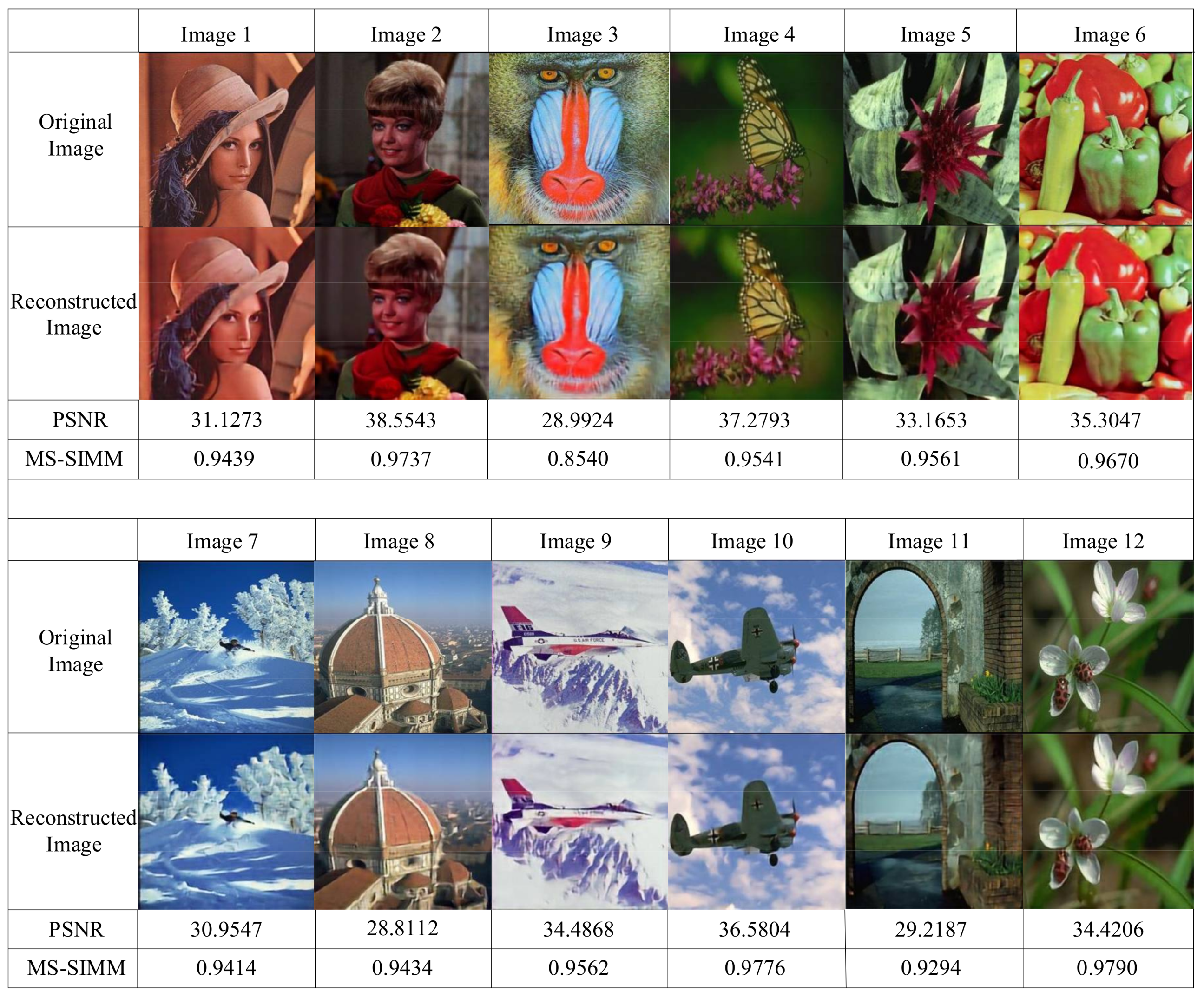
We randomly selected 12 images in the image dataset for testing, and the original and reconstructed images are shown in
Figure 7. The numerical parameters of PSNR and MS-SSIM are also shown under the corresponding image in
Figure 7. By comparison, we can conclude that our implementation of CAE based on FPGA works well and has good image compression and reconstruction effects.
By using Verilog hardware description language, our hardware procedure is synthesized and implemented using the Xilinx Vivado2016.2 design suite (Xilinx, San Jose, CA, USA), which provides a full solution for Xilinx programmable devices. According to the device utilization summary given by the design suite, the utilization of the main hardware resources is shown in
Table 1. With the numbers of network layers and weight parameters set at 13 and 68,227, respectively, we can see that the main resources, such as LUT and FF, take a very small percentage.
Our CPU platform is Intel i7-6700K CPU (Intel, Santa Clara, CA, USA) at 4 GHz with a 16 GB RAM. The GPU platform is NVIDIA GTX TITAN Xp (NVIDIA, Santa Clara, CA, USA). A 150 MHz system clock is used for the framework on FPGA. In the experiment, “time.clock()” instruction of Keras is used to obtain the computing time while running on either CPU or GPU. The computing time of FPGA is calculated by counting the number of clock cycles consumed from input to output. As for the power consumptions of GPU, CPU, and FPGA, they are acquired from the “nvidia-smi” command provided by NVIDIA, the electro-instruments, and the power analyzer integrated in Vivado2016.2, respectively. A performance comparison of FPGA, CPU, and GPU is shown in
Table 2.
As the experimental results show, in terms of compression speed, it consumes 15.73 ms running on FPGA and 115.29 ms running on CPU. In terms of the computing performance per watt, it is 26.49 GOPS/W running on FPGA, which is far beyond that of CPU and GPU.
4. Conclusions
An implementation of CAE based on FPGA is presented in this paper, which newly introduces a periodic layer-multiplexing framework. The encoder part of the proposed CAE framework, which is similar to the decoder, contains five modules, zero padding, a channel distributor, convolutional encoding, a channel arbitrator, and an output controller. In order to enhance the compatibility of the framework and further enhance the speed of convolution calculation, a parallel channels method caching input data and a parallel convolution method based on shift registers are developed, respectively. To evaluate the performance of the CAE framework, an example of image compression is carried out. The experimental results of image compression show that the framework works well and takes up fewer hardware resources, especially as the resource utilization of LUT is just 9.26%. In terms of the compression speed, it consumes 15.73 ms running on FPGA and 115.29 ms running on CPU. In terms of the computing performance per watt, it is 26.49 GOPS/W running on FPGA, which is far beyond that of CPU and GPU. In future work, more multiplexing techniques, like encoder multiplexing, can be adopted to enhance the CAE performance.


