A Multi-Objective Scheduling Optimization Model for a Multi-Energy Complementary System Considering Different Operation Strategies

Abstract

In order to reduce the amount of abandoned clean energy, the complementary characterization of wind power plants (WPPs), photovoltaic power plants (PVs), hydropower stations (HSs), and thermal power plants (TPPs) combined with energy storage devices (ESDs) is considered, and they are integrated into a multi-energy complementary system (MECS). Firstly, a scenario-generating technique is proposed for uncertainty factors using the Wasserstein method and the improved K-medoids theory. Then, a multi-objective model and solution algorithm are constructed under the objectives of attaining the maximum operation revenue, the minimum abandoned energy cost, and the minimum output fluctuations. Meanwhile, the influence of different ESD operation modes on MECS operation is discussed, specifically, the longest life cycle (LLC) and the optimum economic efficiency (OEE). Thirdly, in order to solve the multi-objective model, a solution algorithm is proposed by using the rough set method to convert the multi-objective model into a single objective model based on the payoff table. Moreover, the complementary features of the MECS are evaluated in terms of the load tracking degree, HS secondary peaking capacity, and units of coal consumption. Finally, the improved IEEE 14-bus system is chosen for the simulation analysis. The results show that (1) the proposed uncertainty simulation method can efficiently generate the most representative scenarios; (2) MECSs can utilize complementary power sources, the OEE mode can better optimize MECS scheduling, and the LLC mode can ensure the ESDs’ life cycles; (3) the scheduling scheme of MECS operation reach the optimal level when the capacity ratio of ESD:WPP–PV iso [0.62, 0.77] in the OEE mode and [1, 1.08] in the LLC mode on a typical summer day, and the ratio is [0.92, 1] in the OEE mode and [1.23, 1.31] in the LLC mode on a typical winter day. Therefore, the proposed model provides effective decision-making support for designing the optimal plan for MECS operation.

1. Introduction

The rapid development of the Chinese economy has resulted in a sharp increase in energy consumption. However, China’s fossil-based energy consumption structure has also brought about a severe energy crisis as well as environmental issues. The optimization of the energy consumption structure has already been shown to be an important method for alleviating the above contradiction [1]. Consequently, the importance of wind, solar, and other green renewable energy sources has become increasingly prominent. The Chinese government recently implemented numerous monetary compensation policies to guarantee the sustainable development of renewable energy [2]. The cumulative installed capacities of wind power and photovoltaic power had already reached 169 × 10⁶ kW and 77.42 × 10⁶ kW, respectively in 2016. However, owing to the obvious uncertainty and volatility of wind power and solar power, the retained generation of power should be abandoned to ensure stable system operation [3]. In only the first half of 2017, the total abandoned wind and photovoltaic power generation reached 23.5 × 10⁹ kW·h and 3.7 × 10⁹ kW·h, respectively. Obviously, the solution to the abandoned energy problem has already become an important issue for the promotion of clean energy development and the optimization of the energy consumption structure.

Because to the grid-connected system of uncontrollable power sources brings great challenges to the stable operation of power systems, three available research methods have been adopted by domestic and foreign scholars and workers, namely, improving the forecast accuracy, improving energy storage device (ESD) technology, and utilizing complementary power sources [4]. Firstly, improving the forecast accuracy of uncontrollable clean power sources could reduce the output deviation of power generation. Song et al. [5] designed a new forecast model with an advanced intelligent algorithm, a data preprocessing technique, and a non-negative constraint theory. Mojtaba et al. [6] applied the mixture models of Kohonen’s self-organizing map and the radial basis functions as the clustering method and the classification method, respectively. Then, ESD could reduce the fluctuations of the power output of intermittent clean energy by utilizing the characteristics of discharging-charging power [7]. Kim et al. [8] designed a new distributed energy generation system by integrating renewable power, air energy storage, and natural gas combustion. Atherton et al. [9] analyzed the feasibility of economics and technology when ESDs are applied to a wind farm. Furthermore, Tan et al. [10] discussed the collaborative synthetic effect of ESDs and the demand response in promoting clean energy power generation. The above forecast methods have already been used in practical applications; however, the achievement of high accuracy relies on having an excessively large amount of data, which limits the application space. Meanwhile, ESDs could promote the output of the uncontrollable power source; however, the high investment costs limit the actual application space. Therefore, determining how to utilize complementary but different power sources is key for improving the reliability of the power supply.

Correspondingly, developing an optimal capacity configuration scheme for wind power, photovoltaic power, and conventional power sources could better utilize the complementary characteristics of different power sources [11]. Derrouazin et al. [12] developed a multi-input–output fuzzy logic smart controller to achieve the optimal plan for a hybrid power system. Zhang et al. [13] constructed a short-term optimal scheduling model for a hybrid power system with wind power plants WPP and photovoltaic power plants (PV). Hassan et al. [14] put forward a new hybrid power system including WPP, PV, and fuel cell power generation. Mason [15] proposed a capacity configuration model for small-island electricity systems with WPP, PV, and ESDs. Similarly, Ghada et al. [16] proposed a hybrid generation system with WPP, PV, and flywheel energy storage systems. Iman et al. [17] discussed the influence of the synergic operation of WPP, HS, and PV on net power output curve smoothing. Okan et al. [18] put forward a new energy coordinated model for a virtual power plant and discussed the impact of plug-in hybrid vehicles with a high proportion of wind power penetration. Kaabeche et al. [19] constructed an optimization configuration model for a WPP–PV hybrid energy system and analyzed its economy and reliability. These studies have demonstrated the significance of complementary power sources. Aboelsood et al. [20] chose WPP, solar collectors (SC), combined heat, and ESDs to get the optimal operation cost. The above research discussed the optimal capacity planning configuration and coordinated control of hybrid energy systems with different power sources; however, the complementarity of different power sources from the scheduling perspective needs to be discussed further.

According to the above analysis, some research has already investigated the randomness and intermittent nature of uncontrollable power sources with the three proposed available ways. Firstly, a series of advanced intelligent methods were put forward to improve the forecast accuracy and achieve a better practical effect. However, an excessively large amount of data is needed to achieve high accuracy which consumes too much effort. In order to overcome the above problem, the uncertainty could be simulated by a random sampling technique based on the probability distributions of different uncertainty factors. Secondly, some of the literature has discussed the optimization effect of ESDs on multi-energy complementary system (MECS) operation, and different optimization models have been constructed. However, almost all studies have assumed that the ESDs will fully respond to MECS scheduling to achieve the maximum use of clean energy without considering the influences of different operation modes. In fact, ESD could operate in two modes, namely, the longest life cycle (LLC) and the optimum economic efficiency (OEE). The optimal scheduling strategy of MECS operation will show great differences under different operation modes. That means that a discussion about ESDs’ operation modes is necessary. Finally, most of the research studied the optimal capacity planning configuration and coordinated control of hybrid energy systems and analyzed the complementarity characteristics of different power sources. However, the studied hybrid systems have been limited to only two or three power sources. In fact, WPP, photovoltaic power plants (PV), hydropower stations (HS), thermal power plants (TPP), and energy storage devices (ESDs) show a great complementarity. Therefore, it is important to construct a new hybrid system with the above power sources and discuss the optimal operation strategy. All the above analyses motivated us to develop a multi-objective scheduling optimization model for MECS operation. The main works of the paper are summarized as follows:

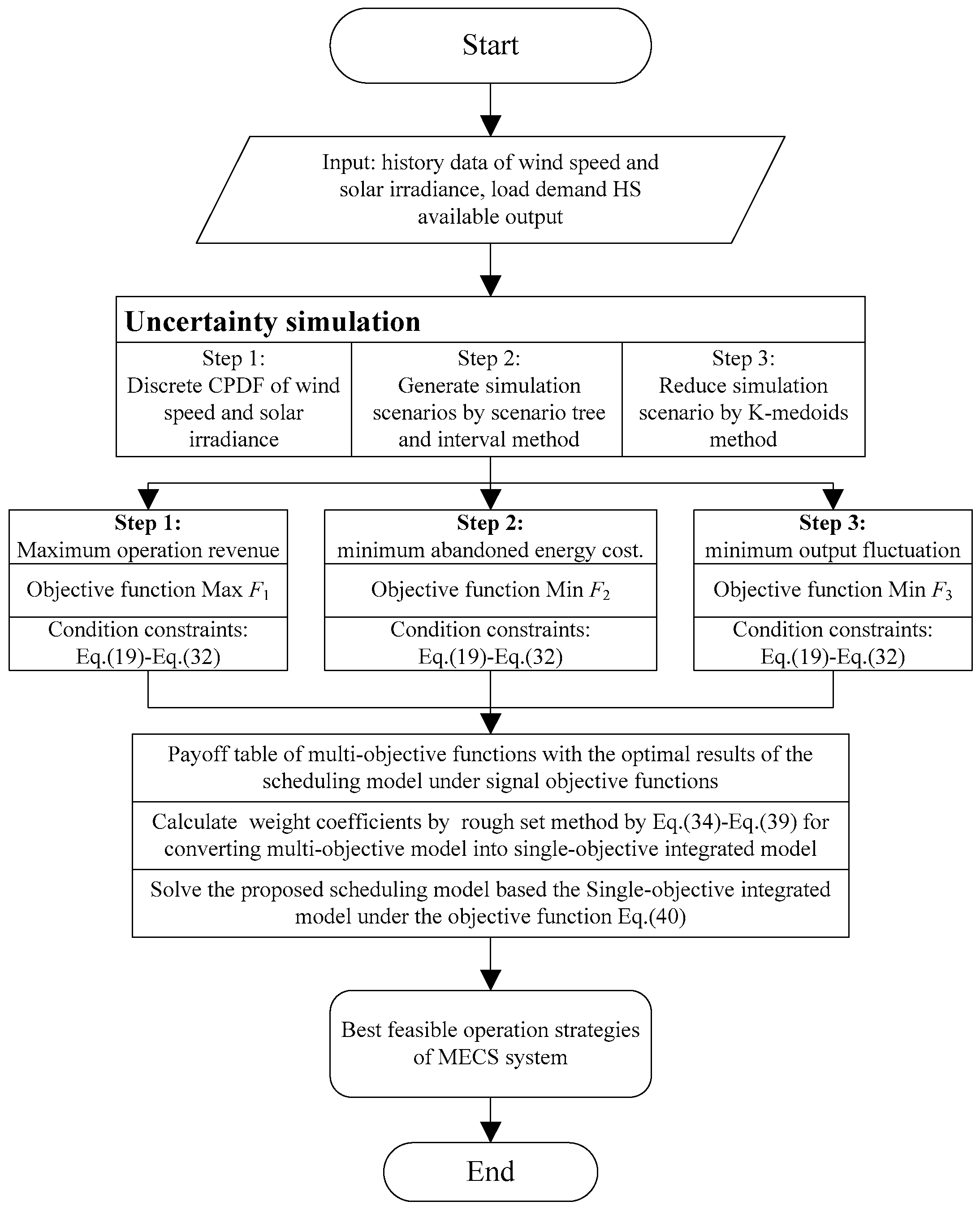
• An uncertainty analysis and simulation method are proposed to generate a typical distribution scenario for the uncertainty factors of MECS operation based on the Wasserstein method, and the K-distance and the K-medoids algorithms. The method includes three steps, namely, the discretization of the continuous probability distribution functions, the generation of the initial simulation scenarios, and the selection of the most representative scenarios.
• A multi-objective scheduling model and solution algorithm are proposed by considering different ESD operation modes under three objective functions, namely, the maximum operation revenue, the minimum abandoned energy cost, and the minimum output fluctuations. Then, the multi-objective model is weighted into the single objective mode by the rough set theory based on the payoff table.
• A complementary evaluation index system is given to evaluate the optimal degree for the whole MECS operation, including the load tracking degree, the HS secondary peaking capacity, and TPP units of coal consumption. The optimal capacity ratios of ESD:WPP and ESD:PV are calculated by a sensitivity analysis to provide reliable decision-making support.

The rest of the paper is organized as follows: Section 2 presents the basic structure of MECS, and Section 3 constructs an uncertainty analysis and simulation method. Then, a multi-objective optimization model for MECS operation is proposed, and a three-step solution algorithm is constructed based on the payoff table and the rough set theory in Section 4. Section 5 chooses the load tracking degree, HS secondary peaking capacity, and TPP units of coal consumption as the complementarity indexes. Furthermore, the improved IEEE14 bus system is used as a simulation system in Section 6. Section 7 highlights the conclusions of the paper.

2. MECS Structure Description

WPPs and PVs (or HSs) are significantly complementary. The output of WPPs is low in the daytime, whereas the output of PVs is high. The output of WPPs is high at night-time (or in rainy weather), whereas the output of PVs is low. Similarly, the output of WPPs is lowest in the summer and highest in the winter and spring, and the output of HSs is highest in summer and lowest in winter [21]. Therefore, the complementary power generation (CPG) of WPPs and PVs ensures a continuous power supply, whereas the CPG of WPPs and HSs could exploit more wind power and improve the HS peaking capacity. Moreover, TPPs could handle the output fluctuations of WPPs and PVs. The bundling operation of WPPs, PVs, and TPPs could smooth out the output curve. As the short-term operation characteristics of WPPs, PVs, HSs, and TPPs exhibit great differences and a strong complementarity, a sensible joint operation scheduling could result in significant comprehensive benefits.

In this study, a MECS is proposed by integrating WPPs, PVs, TPPs, HSs, and ESDs. For analyzing the complementary of different power sources, the paper assumes all the power sources are independent. Then, the MECS is controlled by an independent operation center (IOC) based on the prediction of weather conditions, which is priority-scheduled to meet terminal customer load demand. The surplus output of the MECS can be transferred to other regions to earn more economic revenue. Moreover, when the available output of MECS cannot meet the load demand, the IOC can purchase power from a generation company (GC). Figure 1 shows the basic structure of the MECS operation.

In the MECS, the WPP and the PV are uncontrolled power sources, whereas the HS, the TPP, and the ESD are controlled power sources. The ESD charges when the load demand is lower than the available power output; otherwise, the ESD discharges (when the load demand is higher than the actual power output). In this study, the maximum benefits, the minimum abandoned energy, and the minimum output fluctuations of the MECS operation are taken as the objective functions for obtaining comprehensive scheduling optimization.

3. Uncertainty Analysis and Simulation

3.1. Uncertainty Analysis

In general, the uncertainties of a power system mainly come from two aspects: the power sources and the load demand. For the uncertainties from the load demand side, the load prediction deviation can be described by a normal distribution function. Then, the distribution functions for load demand will also follow a normal distribution function. During the day-ahead scheduling, HS, TPP, and ESD could all provide a reserve service for the load demand. Furthermore, daily weather forecasting technology is mature, so the think power system can better cope with the uncertainty of the load demand. In particular, as smart grid technology becomes more and more advanced, the demand response will be another resource that can be used to overcome the uncertainty from load demand.

The uncertainties from the power source side are mainly caused by uncontrollable clean energy sources, such as wind power and photovoltaic power. The outputs of WPP and PV are not controllable because the natural wind speed and solar irradiance are influenced by the weather conditions. The output of HS is uncertain from the perspective of the seasonal characteristics, and it is controllable from the perspective of the complementary energy characteristics. If the TPP output is sufficient to offset the insufficient output of HS, the uncertainty of the HS output can be ignored. Therefore, this paper mainly discusses the uncertainties due to WPP and PV.

3.2. Uncertainty Model

Based on the above analysis, only the uncertainties from WPP and PV are considered. In order to simulate the uncertainties, suitable probability distribution functions are needed. Once the simulation results of the wind speed and solar irradiance have been attained, the power outputs of WPP and PV can be calculated.

(1) WPP Uncertainty Model

The output of WPP has a high level of uncertainty. The simulation of wind speed is the key to calculating the output of WPP. It has been proven that the Rayleigh distribution function can be used to simulate wind speed as follows:

$$f\left(v_t\right)=\frac{{\phi }_t}{{\vartheta }_t}{\left(\frac{v_t}{{\vartheta }_t}\right)}^{{\phi }_t-1}{e}^{-{\left(v_t/{\vartheta }_t\right)}^{{\phi }_t}}$$

(1)

where $v_t$ is the wind speed at time t. ${\phi }_t$ and ${\vartheta }_t$ are the shape factor and the scale factor at time t. Then, the WPP output can be calculated by Equation (2), as follows:

$$g_{WPP,t}^{\ast }=\{\begin{array}{l}0,\hspace{1em}\hspace{1em}\hspace{1em}\hspace{1em}\hspace{1em}\hspace{1em}0\le v_t<v_{in}, v_t>v_{out}\\ \frac{v_t-v_{in}}{v_{rated}-v_{in}}{g}_R,\hspace{1em}\hspace{1em}{v}_{in}\le v_t\le v_{rated}\\ g_R,\hspace{1em}\hspace{1em}\hspace{1em}\hspace{1em}\hspace{1em} v_{rated}\le v_t\le v_{out}\end{array}$$

(2)

where $g_{WPP,t}^{\ast }$ is the available output of the WPP at time t. $g_R$ is the rated output of WPP. $v_t$ is the real-time wind speed at time t. $v_{in}$, $v_{out}$ and $v_{rated}$ are the cut-in, cut-out, and rated speeds, respectively.

(2) PV uncertainty model

Similarly, existing research has proven that the beta distribution function can be used to describe solar irradiance as follows:

$$f\left({\theta }_t\right)=\{\begin{array}{l}\frac{\Gamma \left({\alpha }_t\right)\Gamma \left({\beta }_t\right)}{\Gamma \left({\alpha }_t\right)+\Gamma \left({\beta }_t\right)}{\theta }^{{\alpha }_t-1}{\left(1-{\theta }_t\right)}^{{\beta }_t-1}, 0\le {\theta }_t\le 1,{\alpha }_t\ge 0,{\beta }_t\ge 0\\ 0\hspace{1em}\hspace{1em}\hspace{1em}\hspace{1em}\hspace{1em}\hspace{1em}\hspace{1em}\hspace{1em}\hspace{1em}\hspace{1em},otherwise\end{array}$$

(3)

where ${\theta }_t$ is the solar irradiance at time t. ${\alpha }_t$ and ${\beta }_t$ are the shape parameters of the beta distribution at time t, which can be calculated by the mean value and the standard deviation of irradiance [15]. After simulating the solar irradiance, the PV output can be calculated as follows:

$$g_{PV,t}^{\ast }={\eta }_{PV}\times S_{PV}\times {\theta }_t$$

(4)

where $g_{PV,t}^{\ast }$ is the available output of PV at time t. ${\eta }_{PV}$ and $S_{PV}$ are the efficiency and total area, respectively. ${\theta }_t$ is the solar radiation intensity at time t.

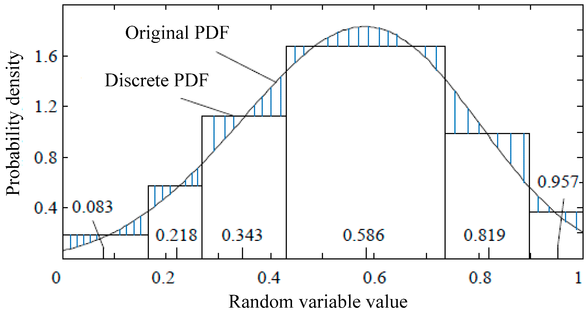
3.3. Uncertainty Simulation

The PDFs of the WPP output, PV output, and load are continuous probability distribution functions (CPDFs). In general, discrete PDFs are required for MECS scheduling. Therefore, a discretization process for continuous PDFs must be completed before the uncertainty simulation. Thus, the uncertainty simulation comprises three steps: PDF discretization, scenario simulation, and scenario reduction.

(1) PDF discretization

The discretization process involves dividing the continuous function curve into a number of segments corresponding to certain intervals. In general, these intervals can be equal or unequal. In the former case, all scenarios can be considered, and, in fact, the probabilities of some scenarios may not reflect the real probabilities. In the latter case, the probability can be captured more accurately. In this study, the Wasserstein method is adopted for the discretization of PDFs. More details on this method may be found in Reference [22].

It is assumed that $f_{\mathrm{c}}\left(x\right)$ is a CPDF to be discretized using N points. Then, the optimal discrete points $z_n\left(n=1,2,\dots ,N\right)$ under the Wasserstein distance indicator are obtained by

$${\displaystyle {\int }_{-\infty }^{z_n}{f}_{\mathrm{c}}{\left(x\right)}^{1/(1+r)}dx=\frac{2n-1}{2N}}{\displaystyle {\int }_{-\infty }^{\infty }{f}_{\mathrm{c}}{\left(x\right)}^{1/(1+r)}dx}.$$

(5)

Then, the discrete probability of $z_n$ is calculated as follows:

$$p_d^n={\displaystyle {\int }_{\frac{z_{n-1}+z_n}{2}}^{\frac{z_n+z_{n+1}}{2}}{f}_{\mathrm{c}}{\left(x\right)}^{1/(1+r)}dx},n=1,2,\dots ,N$$

(6)

where $p_d^n$ represents the discrete probability of $z_n$. When n = 0, $p_d^0$ represents the lower bound of the variable x, and its value is $p_d^0={\displaystyle {\int }_{z_0}^{\frac{z_1+z_2}{2}}{f}_{\mathrm{c}}\left(x\right)dx}$. When n = N + 1, $p_d^{N+1}$ represents the upper bound of x, and its value is equal to ${\displaystyle {\int }_{\frac{z_{Q-1}+z_Q}{2}}^{z_{Q+1}}{f}_{\mathrm{c}}\left(x\right)dx}$. By combining Equations (1) and (3) with Equation (6), the optimal discrete points can be calculated. Correspondingly, the discrete PDFs for the outputs of the WPP, PV, and load can be obtained for the scenario simulation. Figure 2 shows the discretization process (6 discrete points).

(2) Scenario simulation

After the PDFs of the WPP output, PV output, and load have been discretized, the simulation scenarios can be obtained by a sampling method, such as Monte Carlo or Latin hypercube sampling. Monte Carlo is highly versatile and accurate. When the distribution has low probability regions, small samples are generally not representative. The Latin hypercube sampling method divides the PDF into several equal intervals to obtain the sample from each interval [12]. However, the probabilities of some scenarios may not reflect the real probabilities [23]. Based on the above analysis, in this study, the Wasserstein method is used to divide the continuous probability distribution curves. Then, the scenario tree method is used to describe the different states of power output, namely, the high, mean, and low (z = 1, 2, 3, respectively). In Equation (5), the optimal discrete points for the WPP and PV outputs are calculated and the simulation interval of the PDF is accordingly divided. The simulation scenario set is gained by using the interval simulation method. Then, we assume $g_t^z$ is the expected output in each state at time t. Equation (6) yields the probability $p_t^z$ of simulation scenarios in each state at time t. Consequently, the scenario set and probability are $S=\left\{g_t^z|t=1,2,\dots ,T\right\}$ and $p={\displaystyle \prod _{t\in T}{p}_t^z}$, respectively. More details on the scenario simulation can be found in [24].

(3) Scenario reduction

After the continuous distributions of the random variables have been optimally discretized in each period, the scenario set formed by the entire scheduling interval is large, which results in dimension explosion. If all scenarios are applied to make the optimal scheduling scheme, the effort required to solve the proposed mode will be large. The number of simulation scenarios will determine the number of model iteration calculations. If the scenarios are not reduced, some approximate repeated calculations will occur when some scenarios are similar. However, if the number of scenarios is reduced and the most representative scenarios are chosen, then the scenario reduction will decrease the calculation effort. Based on the above analysis, some scenarios with high similarity should be deleted. The main theory of scenario reduction involves deleting similar scenarios by comparing each scenario with the other scenarios. Correspondingly, this paper uses the K-distance method to measure the distances of different scenarios to delete redundant scenarios [25]. It is assumed that $d\left(u^s,u^k\right)$ is the distance between scenarios $u^s$ and $u^k$ in scenario set S. If scenario set K is used to replace the original scenario set with k scenarios, $d\left(u^s,u^k\right)$ is calculated in Equation (7):

$$d\left(u^s,u^k\right)={\left[{\displaystyle \sum _{t=1}^T{\left(u^s,u^k\right)}^2}\right]}^{1/2}.$$

(7)

Then, we let $q_k$ and $p_s$ be the probabilities of scenario k and scenario s, respectively. The optimal scenario set K should follow the same principle, namely, the probability information should be closest to S.

$$\min {\displaystyle \sum _{u^s\in S,u^s\notin K}{p}_s\underset{u^k\in K}{\min }d\left(u^s,u^k\right)}=\min \inf \left\{\begin{array}{l}{\displaystyle \sum _{s=1}^S{\displaystyle \sum _{k=1}^K{\eta }_{sk}d\left(u^s,u^k\right):{\eta }_{sk}\ge 0},}\\ {\displaystyle \sum _{s=1}^S{\eta }_{sk}=q_k},{\displaystyle \sum _{k=1}^K{\eta }_{sk}=p_s},\forall s,\forall k\end{array}\right\}.$$

(8)

In traditional K-medoids methods, scenario $u^s$ is compared with each scenario $u^k$ to order the group of scenarios closest to $u^s$, which requires a large amount of calculation [26]. In this study, the relative distance across which the ordering is performed is constructed through a comparison with the same reference point $u^0\left(u^0=0\right)$. The detailed process of sorting and grouping can be found in Reference [27]. After the group order has been obtained, $u^0$ should be updated by

$$u^l=u^k\in \arg \underset{u^l\in K}{\min }d\left(u_{mid}^l,u^k\right)$$

(9)

$$u_{mid}^l={\displaystyle \sum _{u^s\in S}{p}_s{u}^s}/{\displaystyle \sum _{u^s\in S}{p}_s}$$

(10)

where $u^l$ is the updated clustering center. Then, the updated ${\displaystyle \sum _{u^s\in S,u^s\notin K}{p}_s\underset{u^k\in K}{\min }d\left(u^s,u^k\right)}$ is calculated, and if the value meets the requirements, the final reduced scenario set is obtained. Otherwise, the updated clustering center needs to be updated again. To improve the calculation speed, the simultaneous backward technique is applied to the scenario reduction process. Figure 3 shows the uncertainty simulation flowchart.

4. Multi-Objective Scheduling Optimization Model

4.1. Multi-Objective Scheduling Model

To satisfy different operational requirements and consider different benefits, the maximum operation revenue, the minimum abandoned energy cost, and the minimum output fluctuations were chosen as the MECS operation objectives in this study.

4.1.1. Objective Functions

MECSs can utilize the complementarity of different power sources, make full use of the adjustable power sources’ peaking capacities, and promote the grid connection of clean energy sources, such as wind and photovoltaic power. Therefore, the MECS operation revenue comprises the economic revenue, environmental revenue, and peak shaving revenue.

$$\left(\mathrm{P}1\right)\hspace{0.17em}\hspace{0.17em}\hspace{0.17em}\max \hspace{0.17em}{F}_1={\displaystyle \sum _{t=1}^T{\displaystyle \sum _{k=1}^K{\gamma }_k{\left(R_{WPP,t}+R_{PV,t}+R_{ESD,t}+R_{HS,t}+R_{TPP,t}\right)}_k}}$$

(11)

where t is the index for time. k is the index for the scenario. ${\gamma }_k$ is the probability of scenario k. $R_{WPP,t}$, $R_{PV,t}$, $R_{ESS,t}$, $R_{HS,t}$, and $R_{G,t}$ denote the operation revenue for the WPP, the PV, the ESD, the HS, and the TPP at time t, respectively. The operation revenue for the WPP, the PV, and the ESD have already been studied in Reference [10]. As is the case with the WPP and the PV, the cost of the initial investment, operation, and maintenance of the HS is classified as the sunk cost, whereas the energy consumption cost of the HS can also be ignored. Therefore, the revenue of the HS operation equals the product of the power price and power output. Thus, the revenue of the TPP operation comprises three parts: the power generation cost, the startup–shutdown cost, and the pollutant emission cost. The detailed calculations are as follows:

$$R_{TPP,t}={\rho }_{TPP,t}{g}_{TPP,t}-{\rho }_{\mathrm{coal}}\left({\pi }_{TPP,t}^{pg}+{\pi }_{TPP,t}^{ss}\right)-{\pi }_{TPP,t}^{pe}$$

(12)

$${\pi }_{TPP,t}^{pg}=a_{TPP}+b_{TPP}{g}_{TPP}+c_{TPP}{\left(g_{TPP,t}\right)}^2$$

(13)

$${\pi }_{TPP,t}^{ss}=\left[u_{TPP,t}(1-u_{TPP,t})\right]\cdot \{\begin{array}{l}{N}_{CGT}^{hot},T_{CGT}^{\min }<T_{CGT,t}^{\mathrm{off}}\le T_{CGT}^{\min }+T_{CGT}^{cold}\\ N_{CGT}^{cold},T_{CGT,t}^{\mathrm{off}}>T_{CGT}^{\min }+T_{CGT}^{cold}\end{array}$$

(14)

$${\pi }_{TPP,t}^{pe}={\displaystyle \sum _{e=1}^E{p}_e\left[{\tilde{a}}_{TPP}^e+{\tilde{b}}_{TPP}^e{g}_{TPP}+{\tilde{c}}_{TPP}^e{\left(g_{TPP,t}\right)}^2\right]}$$

(15)

where ${\pi }_{TPP,t}^{pg}$, ${\pi }_{TPP,t}^{ss}$, and ${\pi }_{TPP,t}^{pe}$ denote the power generation cost, startup–shutdown cost, and pollutant emissions cost of the TPP at time t, respectively. $a_{TPP}$, $b_{TPP}$, and $c_{TPP}$ are the cost coefficients of the TPP power generation. ${\rho }_{\mathrm{coal}}$ is the coal price. $u_{TPP,t}$ and $D_{TPP,t}$ are the status and cost of the TPP startup–shutdown at time t. $N_{TPP}^{cold}$ and $N_{TPP}^{hot}$ are startup costs of the TPP operation in the cold mode and hot mode. $T_{TPP}^{\min }$ and $T_{CGT,t}^{\mathrm{off}}$ are the minimum allowable and continuous downtime of TPP at time t, respectively. $T_{TPP}^{cold}$ is the required time for TPP startup in cold-start mode. $a_{TPP}$, $b_{TPP}$, and $c_{TPP}$ are the cost coefficients of TPP power generation.

$$\left(\mathrm{P}2\right)\hspace{0.17em}\hspace{0.17em}\min \hspace{0.17em}\hspace{0.17em}{F}_2={\displaystyle \sum _{t=1}^T{\displaystyle \sum _{k=1}^K{\gamma }_k{\left[{\rho }_{WPP,t}\left(g_{WPP,t}^{\ast }-g_{WPP,t}\right)+{\rho }_{PV,t}\left(g_{PV,t}^{\ast }-g_{PV,t}\right)+{\rho }_{HS,t}\left(g_{HS,t}^{\ast }-g_{HS,t}\right)\right]}_k}}$$

(16)

where, $F_2$ is the abandoned energy cost of WPP, PV, and HS during the scheduling period. For MECS, determining how to use the complementary characteristics of different power sources is the key to reducing the amount of abandoned energy. In fact, if the abandoned energy could be absorbed, more economic revenue could be gained. Correspondingly, this part of the economic revenue can be regarded as the opportunity cost. ${\rho }_{WPP,t}$, ${\rho }_{PV,t}$, and ${\rho }_{HS,t}$ are the power prices of WPP, PV, and HS, respectively, at time t. $g_{WPP}^{\ast }$, $g_{PV}^{\ast }$, and $g_{HS,t}^{\ast }$ are the available outputs of WPP, PV, and HS at time t, respectively.

$$\left(\mathrm{P}3\right)\hspace{0.17em}\hspace{0.17em}\min \hspace{0.17em}{F}_3={\left\{{\displaystyle \sum _{k=1}^K{\gamma }_k}{\left\{{\displaystyle \sum _{t=1}^T{\left[g_{WPP,t}+g_{PV,t}-\left(g_{ESD,t}^{dis}-g_{ESD,t}^{ch}\right)-g_{av}\right]}^2}\right\}}_k\right\}}^{1/2}/T$$

(17)

$$g_{av}={\displaystyle \sum _{t=1}^T\left[g_{WPP,t}+g_{PV,t}-\left(g_{ESD,t}^{dis}-g_{ESD,t}^{ch}\right)\right]/T}$$

(18)

where $g_{av}$ is the average value of the MECS power output fluctuations. For the MECS, the uncertainties of WPP and PV will bring a great level of uncertainty in the net power output. Therefore, determining how to measure the power output fluctuations is key to guaranteeing the stable operation of the MECS. In the MECS, ESD could charge the power of WPP and PV in the valley period and discharge their power in the peak period. Therefore, the standard deviation of the total net power output of WPP and PV is taken as the measure indicator. $g_{ESD,t}^{dis}$ and $g_{ESD,t}^{ch}$ are the power levels of ESD discharging-charging at time t, respectively. $F_3$ is the standard deviation of the power output fluctuations of the MECS. When $F_3$ is small, the output fluctuations of the WPP and PV are small, which is more favorable for the safe operation of the MECS.

4.1.2. Constraint Conditions

To ensure the safe and stable operation of the MECS, some necessary constraint conditions should be considered, for example, the load supply and demand balance constraints, the TPP operation constraints, the ESD operation constraints, and the system reserve constraints. A detailed description of the MECS operation constraints is as follows.

(1) Supply and demand balance constraint

$$\underset{MECS\hspace{0.17em}output\hspace{0.17em}}{\underbrace{\left[g_{WPP,t}\left(1-{\phi }_{WPP}\right)+g_{PV,t}\left(1-{\phi }_{PV}\right)+\left(g_{ESD,t}^{dis}-g_{ESD,t}^{ch}\right)+g_{HS,t}\left(1-{\phi }_{HS}\right)+g_{TPP,t}\left(1-{\phi }_{TPP}\right)\right]}}+g_{GC,t}=L_t$$

(19)

where ${\phi }_{WPP}$, ${\phi }_{PV}$, ${\phi }_{HS}$, and ${\phi }_{TPP}$ are the power loss rates of the WPP, PV, HS, and TPP, respectively. $g_{GC,t}$ is the exchange power from the GC at time t. When $g_{GC,t}$ is positive, the MECS will purchase power from the GC to satisfy its power demand. When the $g_{GC,t}$ is negative, the MECS will transfer surplus power to the utility grid.

(2) HS power output constraint

$$g_{HS,t}={\rho }_{HS}^0+{\rho }_{HS}^1{Q}_{HS,t}+{\rho }_{HS}^2{V}_{HS,t}^{}+{\rho }_{HS}^3{Q}_{HS,t}{V}_{HS,t}^{}+{\rho }_{HS}^4{Q}_{HS,t}^2+{\rho }_{HS}^5{V}_{HS,t}^2+\epsilon$$

(20)

where $\epsilon$ is an error term calculated by history data, ${\rho }_{HS}^0$, ${\rho }_{HS}^1$, ${\rho }_{HS}^2$, ${\rho }_{HS}^3$, ${\rho }_{HS}^4$, and ${\rho }_{HS}^5$ are the power output coefficients of the HS. $Q_{HS,t}$ and $V_{HS,t}^{}$ are the output capacity and the reservoir capacity of HS at time t.

$$Q_{HS,t}^{\min }\le Q_{HS,t}^{}\le Q_{HS,t}^{\max }$$

(21)

$$V_{HS,t}^{\min }\le V_{HS,t}^{}\le V_{HS,t}^{\max }$$

(22)

where $Q_{HS}^{\min }$ is the minimum water flow for the HS power output. $Q_{HS}^{\max }$ is the maximum water flow for the HS power output. $V_{HS}^{\min }$ is the lower bound of the reservoir capacity. $V_{HS,t}^{\max }$ is the upper bound of the reservoir capacity. The reservoir capacity of the HS at the initial and end time points of the scheduling period should meet the following constraint:

$$V_{HS}^T=V_{HS}^0+{\displaystyle \sum _{t=1}^T[{\stackrel{⌢}{Q}}_t^{}-{\underset{⌣}{Q}}_t^{}-S_{HS,t}+{\displaystyle \sum _{h=1}^H(Q_{h,t-{\tau }_{h,HS}}+S_{h,t-{\tau }_{h,HS}})}]}$$

(23)

where ${\stackrel{⌢}{Q}}_t^{}$ is the water inflow at time t, ${\underset{⌣}{Q}}_t^{}$ is the water outflow at time t. $S_{HS,t}$ is the amount of wastewater at time t, and H is the number of upstream hydropower stations. ${\tau }_h$ is the delayed water flow between the HS and the upstream hydropower station h. $V_{HS}^T$ is the water storage capacity at time T. $V_{HS}^0$ is the water storage capacity at the initial time point. Water runoff into the reservoir comprises the water supply and the outflow from the upstream reservoir, as follows:

$$V_{HS,t}^{}=V_{HS,t}^0+\Delta t{\displaystyle \sum _{\tau =1}^{t-1}({\stackrel{⌢}{Q}}_{HS,\tau }^{}-Q_{HS,\tau }^{}-S_{HS,\tau }^{}+Q_{HS-1}^{\tau -t_{\mathrm{up}}}+S_{HS-1}^{\tau -t_{\mathrm{up}}})}$$

(24)

where $Q_{HS-1}^{\tau -t_{\mathrm{up}}}$ and $S_{HS-1}^{\tau -t_{\mathrm{up}}}$ are the power generation flow and wastewater flow, respectively, of the upstream hydropower station. $t_{\mathrm{up}}$ is the time lag corresponding to the flow from the upstream hydropower station to the downstream hydropower station.

(3) ESD operation constraints

The ESD can complementarily operate with the WPP and the PV by utilizing its discharge–charge cycle. Two operation modes exist, namely, the longest life cycle (LLC) mode and the optimum economic efficiency (OEE) mode. Thus, the main constraints are as follows:

$${\displaystyle \sum _{t=1}^T(Q_0+g_{ESD,t}^{ch}-Q_t)}(1-{\rho }_{ESD})={\displaystyle \sum _{t=1}^T{g}_{ESD,t}^{dis}}$$

(25)

$$0\le g_{ESD,t}^{ch}\le {\overline{g}}_{ESD,t}^{ch}$$

(26)

$$0\le g_{ESD,t}^{dis}\le {\overline{g}}_{ESD,t}^{dis}$$

(27)

where ${\overline{g}}_{ESS,t}^{ch}$ and ${\overline{g}}_{ESS,t}^{dis}$ are the upper bounds for ESS charging–discharging at time t, respectively.

$$Q_{t+1}=\{\begin{array}{l}{Q}_t-g_{ESS,t}^{dis}\left(1+{\rho }_{ESS,t}^{dis}\right),\hspace{0.17em}during discharge\\ Q_t+g_{ESS,t}^{ch}\left(1-{\rho }_{ESS,t}^{ch}\right),\hspace{0.17em}during charge\end{array}$$

(28)

where ${\rho }_{ESS,t}^{dis}$ and ${\rho }_{ESS,t}^{ch}$ are the power loss rates of the ESD during discharge and charge, respectively, at time t. The main objectives of LLC are to optimize the ESD’s discharge–charge cycles, improve the ESD’s operation life, and simultaneously increase the system’s peak shaving capacity. That is,

$$g_{ESD,t}^{ch}\to g_{ESD}^{ch,\mathrm{R}}$$

(29)

$$g_{ESD,t}^{dis}\to g_{ESD}^{dis,\mathrm{R}}$$

(30)

$$g_{ESD,t}^{ch}\cdot g_{ESD,t}^{dis}=0$$

(31)

where $g_{ESS,t}^{chr,\mathrm{R}}$ and $g_{ESS,t}^{dis,\mathrm{R}}$ are the rated power levels of the ESD charge and discharge, respectively.

(4) System reserve constraints:

$$\left(g_{TPP,t}^{\max }-g_{TPP,t}^{}\right)+\left(g_{HS,t}^{\max }-g_{HS,t}^{}\right)\ge r_1\cdot L_t+r_2\cdot g_{WPP,t}+r_3\cdot g_{PV,t}$$

(32)

$$\left(g_{TPP,t}^{}-g_{TPP,t}^{\min }\right)+\left(g_{HS,t}^{}-g_{HS,t}^{\min }\right)\ge r_4\cdot g_{WPP,t}+r_5\cdot g_{PV,t}$$

(33)

where $g_{TPP,t}^{\max }$ and $g_{HS,t}^{\max }$ are the maximum outputs of the TPP and the HS at time t, respectively. $g_{TPP,t}^{\min }$ and $g_{HS,t}^{\min }$ are the minimum outputs of the TPP and HS at time t, respectively. $r_i\left(i=1,2,3,4,5\right)$ represents the up reserve coefficients of the load, WPP, and PV and the down reserve coefficients of the WPP and PV, respectively.

(5) Other power source constraints

In the MECS, the other power sources are the TPP, the WPP, and the PV. The operation constraints of the WPP and the PV should satisfy the maximum output constraints, namely, the outputs of the WPP and the PV should not be greater than the system’s allowable output, which has already been studied in Reference [21]. The constraints of the TPP operation comprise the maximum/minimum output constraints, the upwards/downwards climbing constraints, and start–shutdown time constraints, which have already been studied in Reference [28].

4.2. Multi-Objective Model Solution

We proposed a multi-objective optimization model for the MECS operation. There are two methods for solving such a model. The first is to solve it using group intelligence algorithms, for example, genetic algorithms, particle swarm algorithms, and ant colony algorithms. As an intelligence algorithm can globally search for the optimal solution, the programming code is excessively complex, particularly in mathematical models with integers and continuous and discrete variables, thus yielding non-optimal results [10].

The second method is to weight multi-objective functions into an integrated single-objective function. In general, the weighted coefficients can be obtained subjectively or via weight determination methods for different objective functions [28]. In a previous study, the weight coefficients were mainly calculated by using the entropy weight method [29]. The applicability of this method is limited by the uncertainty factors and imperfect information existing in the MECS operation. To overcome this problem, this paper uses the rough theory to handle the information in the proposed multi-objective model. The calculation process comprises three steps, namely, the construction of the payoff table, the calculation of the weight coefficients, and the conversion of the multi-objective functions.

4.2.1. Payoff Table

The payoff table mainly reflects the relationships between different objective functions [28]. The values of the objective functions were calculated when the MECS operated under other optimization objectives. Firstly, the optimal scheduling schemes were calculated as individual optimization functions. Then, the values of the other objective functions $F_i,i=1,\dots ,i-1,\dots ,i+1\dots ,I$ were calculated under the optimized objective functions $F_i,i=1,2,\dots ,I$. Assume $F_{ij}^{},j=1,2,\dots ,I$ is the values of the other objectives under $F_i$, and $F_{ii}^{\ast }$ is the optimal value of objective $F_i$. Then, the payoff table can be gained.

Table 1. The payoff table of the proposed multi-objective model.

Functions	${\mathit{F}}_1$	${\mathit{F}}_2$	…	${\mathit{F}}_{\mathbf{I}}$
$F_1$	$F_{11}^{\ast }$	$F_{12}^{}$	…	$F_{1\mathrm{I}}^{}$
$F_2$	$F_{21}^{}$	$F_{22}^{\ast }$		$F_{2\mathrm{I}}^{}$
…	…	…	…	…
$F_I$	$F_{\mathrm{I}1}^{}$	$F_{\mathrm{I}2}^{}$	…	$F_{\mathrm{II}}^{\ast }$

is the payoff table of the proposed multi-objective model.

According to Table 1, the minimum value and the maximum value can be gained for different objective functions. Correspondingly, the information needed to calculate the weight can be collected. Since different objectives have different magnitudes, dimension reduction is necessary before calculating the weight coefficients. The fuzzy satisfaction theory can be used to estimate the optimization degrees of different objective functions [29]. In general, the objective functions exist in two optimization directions, namely, the maximum and the minimum. Therefore, this paper applies the decreasing gradient half membership functions and increasing half line membership functions to handle the objectives.

When the optimization direction of the objective function is in the minimal direction:

$$f_i=\{\begin{array}{l}0,F_i\ge F_i{}^{\max }\\ \frac{F_i{}^{\max }-F_i}{F_i{}^{\max }-F^{\min }},F_i{}^{\min }<F_i<F_i{}^{\max }\\ 1,F_i\le F_i{}^{\min }\end{array}.$$

(34)

When the optimization direction of the objective function is in the maximal direction:

$$f_i=\{\begin{array}{l}1,F_i\ge F_i{}^{\max }\\ \frac{F_i-F_i{}^{\min }}{F_i{}^{\max }-F^{\min }},F_i{}^{\min }<F_i<F_i{}^{\max }\\ 0,F_i\le F_i{}^{\min }\end{array}$$

(35)

where $F_i{}^{\min }$ is the minimum value of the objective function $F_i(\cdot )$. $F_i{}^{\max }$ is the maximum value of the objective function $F_i(\cdot )$. $f_i$ is the membership function.

4.2.2. Weight Calculation

Rough sets can be used to process incomplete and inaccurate data by learning, induction, and excavation and can be transformed into relatively clear and concise data systems to support decision analyses. The detailed theory about the rough set theory is detailed in the literature [26]. When the rough set theory is used to calculate the weight, the weight problem is transformed into a multi-attributed evaluation problem. Correspondingly, the knowledge dependency and attribute importance evaluation methods were constructed for the weight calculations. The detailed process is as follows:

(1) Construction of the relationship data model

It is assumed that the weight coefficient of $f_i$ is $1/\mathrm{I}$. Then, the value of the integrated single objective $\tilde{F}$ can be calculated. $\tilde{F}$ is regarded as a decision attribute, and $D=\left\{\tilde{F}\right\}$ is regarded as a decision attribute set. $u_k$ is the optimal value of the comprehensive objective, which is an information point of the study object F. Obviously, $u_j=(f_{1j},f_{2j},\dots ,f_{mj};{\tilde{F}}_j)$. $U=\left\{u_1,u_2,\dots ,u_j\right\}$ is the main domain, namely, the sample set. Therefore, the attributes of $u_k$ are $f_i(u_j)=v_{ij}$ and $F_i(u_j)={\tilde{F}}_j$. It is assumed that $R_V$ and $R_{\mathrm{D}}$ are knowledge bases.

(2) Calculation of the dependence degree of $R_V$ on $R_{\mathrm{D}}$, that is,

$$r_{R_{\mathrm{V}}}(R_{\mathrm{D}})=\frac{{\displaystyle \sum \rho [R_{\mathrm{V}}({[\tilde{F}]}_{R_{\mathrm{D}}})]}}{\rho (U)}$$

(36)

where $\rho (\cdot )$ represents the set base, and $p_v(D)$ is the knowledge of all individuals using the classification U/C in the universe $U$, which can correctly classify the equivalence classes of object sets in the U/D.

(3) Calculation of the dependence degree of $R_{V-\left|v_i\right|}$ on $R_{\mathrm{D}}$, that is,

$$r_{R_{V-\left|v_i\right|}}(R_{\mathrm{D}})=\frac{{\displaystyle \sum \rho [R_{V-\left|v_i\right|}({[\tilde{F}]}_{R_{\mathrm{D}}})]}}{\rho (U)}$$

(37)

where $p_{V-\left|v_i\right|}(D)$ is the knowledge of all individuals using the classification U/C in the universe $U$ after removing the indicator $V_i$.

(4) Calculation of the weight value of objective i, namely,

$${\sigma }_{\mathrm{D}}(D)=r_{R_V}(D)-r_{R_{V-\left|v_i\right|}}(D)$$

(38)

$${\lambda }_i={\sigma }_{\mathrm{D}}(v_i)/{\displaystyle \sum _{i=1}^I{\sigma }_{\mathrm{D}}(v_i)}$$

(39)

where ${\sigma }_{\mathrm{D}}(D)$ calculates the importance of objective function I. ${\lambda }_i$ is the weight of objective i.

4.2.3. Weighted Single Objective

After getting the weights of the different objective functions, the integrated single objective function can be gained, as shown in Equation (39):

$$\overline{F}=\min \left\{{\displaystyle \sum _{i^{\prime }\in i}{\overline{\lambda }}_{i^{\prime }}\frac{\underset{i^{\prime }}{\max }\left\{F_{i^{\prime }j}^{\ast }\right\}-F_{i^{\prime }}}{\underset{i^{\prime }}{\max }\left\{F_{i^{\prime }j}^{\ast }\right\}-\underset{i^{\prime }}{\min }\left\{F_{i^{\prime }j}^{\ast }\right\}}+{\displaystyle \sum _{i^{″}\in i,i^{″}\ne i^{\prime }}{\overline{\lambda }}_{i^{″}}\frac{f_{i^{″}}-\underset{i^{″}}{\min }\left\{F_{i^{″}j}^{\ast }\right\}}{\underset{i^{″}}{\max }\left\{F_{i^{″}j}^{\ast }\right\}-\underset{i^{″}}{\min }\left\{F_{i^{″}j}^{\ast }\right\}}}}\right\},\left\{i^{\prime }\right\}\cup \left\{i^{″}\right\}=\left\{i\right\}$$

(40)

where ${\overline{\lambda }}_{i^{\prime }}$ and ${\overline{\lambda }}_{i^{″}}$ are the weights of the objective functions with the maximum optimization direction and the minimum optimization direction. The integrated single objective function $\overline{F}$ is thus obtained in Equation (40).

5. Complementarity Evaluation Indexes

MECSs can make full use of the complementarity of different power sources and the peaking capacity of TPP and HS to improve the grid connection of clean energy. In this section, the complementarity evaluation indexes of the MECS are constructed. Moreover, complementation scenarios with different power combinations are considered so that the comprehensive operation benefits of MECSs can be comparatively analyzed. In a previous study [26], the load tracking degree, HS secondary peaking capacity, and TPP unit coal consumption were used as evaluation indexes.

(1) The load tracking degree (LTD)

To fully utilize the complementarity of different power sources, the load tracking degree (LTD) is used to evaluate whether the complementary ratio of power sources is optimal. LTD shows the degree of dispersion of the revised load curve compared with the average value, which can reflect the smoothing effect of the complementary functions of different power sources on the load demand. When the LTD is closer to 1, the capacity of the bundled power output to track the load change is higher and the load curve is smoother [26]. The LTD is defined as

$$\vartheta =\frac{{\displaystyle \sum _{t=1}^T\left(L_t-L_t^{\mathrm{av}}\right)\left(G_{MECS,t}-G_{MECS}^{\mathrm{av}}\right)}}{\sqrt{{\displaystyle \sum _{t=1}^T{\left(L_t-L_t^{\mathrm{av}}\right)}^2}}\sqrt{{\displaystyle \sum _{t=1}^T{\left(G_{MECS,t}-G_{MECS}^{\mathrm{av}}\right)}^2}}}$$

(41)

where $L_t$ represents the load required to absorb the power output of the MECS at time t, $L_t^{\mathrm{av}}$ represents the average load, $G_{MECS,t}$ represents the total output of the MECS at time t, and $G_{MECS,t}^{\mathrm{av}}$ represents the total average output. The load curve may become smoother by optimizing $G_{MECS,t}$, thus making the output curve trend more consistent with $L_t$.

(2) The HS secondary peaking capacity (SPC)

HSs are characterized by low power generation emissions and high regulation, which allow their joint operation with WPPs and PVs. Except for the HS used for the bundling complementary of WPP and PV, the scheduling plan of the other units should be arranged by considering the HSs’ adjustment capability. HSs could be used to perform secondary peaking on the revised load curve, which could promote the load supplied by TPP to be as smooth as possible. This could reduce the start-stop number of TPP and improve the overall operating efficiency. The net load curve for the TPP would be gentler by considering the HSs’ adjustability and, thus, improving the operational efficiency. To distribute the residual load in each period as evenly as possible, the peaking mean square deviation is used to describe the HS peaking capacity. It is defined by

$$\phi =\frac{1}{T}{\left[{\displaystyle \sum _{t=1}^T{\left({\widehat{L}}_t^{}-{\widehat{L}}_t^{\mathrm{av}}\right)}^2}\right]}^{1/2}=\frac{1}{T}{\left\{{{\displaystyle \sum _{t=1}^T\left[\left(L_t^{}-g_{HS,t}-\left(g_{ESD,t}^{dis}-g_{ESD,t}^{ch}\right)\right)-\frac{1}{T}{\displaystyle \sum _{t=1}^T\left(L_t^{}-g_{HS,t}-\left(g_{ESD,t}^{dis}-g_{ESD,t}^{ch}\right)\right)}\right]}}^2\right\}}^{1/2}$$

(42)

where ${\widehat{L}}_t^2$ is the surplus load after removing the HS output, which is equal to $\left(L_t^{}-g_{HS,t}\right)$, and ${\widehat{L}}_t^{\mathrm{av}}$ is the average surplus load after removing the HS output. In general, the load demand curve is gentler when $\phi$ is smaller, thus reducing the start-shutdown frequency and coal consumption.

(3) TPP unit coal consumption

The MECS can fully utilize the regulation characteristics of the hydropower and thermal power units to promote the grid connection of clean energy sources. The large-scale grid connection of clean energy sources could reduce the coal consumption of TPP; correspondingly, the reasonable arrangement of the left load in TPP could reduce coal consumption, which could reduce pollution emission and power generation costs. The power generation unit coal consumption rate $\gamma$ is used to evaluate the operational benefits of the MECS and is defined by

$$\gamma ={\displaystyle \sum _{t=1}^T\left({\pi }_{TPP,t}^{pg}+{\pi }_{TPP,t}^{ss}\right)}/{\displaystyle \sum _{t=1}^T{g}_{TPP,t}}.$$

(43)

6. Simulation Analysis

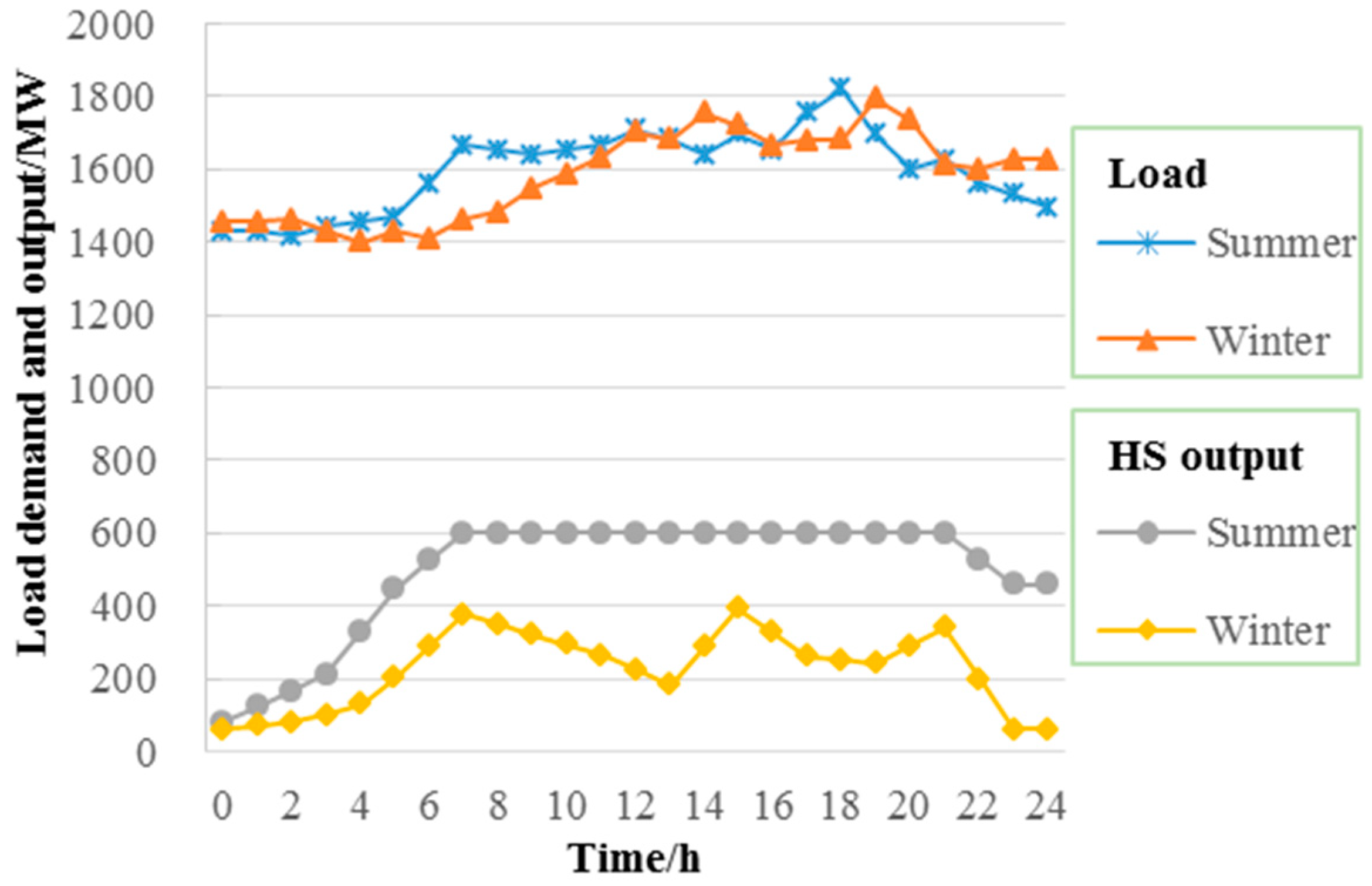
6.1. Basic Data

The improved IEEE 14-bus system with four thermal power units was used as the simulation system [28]. A WPP, a PV, an HS, and ESDs were connected with the simulation system to analyze the complementarity of the different power sources. The rated capacities of the WPP, the PV, and the HS were 900 MW, 400 MW, and 600 MW, respectively. Moreover, 400 MW ESDs were considered to analyze the optimal effects in the OEE and LLC modes. The rated discharge–charge power of the ESDs was 100 MW, the maximum discharge–charge power was 150 MW, and the initial energy storage was zero. The total maximum and minimum loads on a typical load day were 18,500 MW and 1400 MW, respectively, in summer and 1800 MW and 1350 MW, respectively, in winter. The loss of the tested system was 5.5%. The operating parameters and pollutant emission parameters of thermal power units can be found in Reference [25]. Currently, most thermal power tariffs have already included SO₂, NO_x, soot, and other pollutant costs in China; thus, the carbon cost was primarily considered in this study, and the price of CO₂ emission was set to ¥55/ton [29].

Table 2. The key parameters of the thermal power plant (TPP) operation.

Unit	Power Output/MW		Climbing Output/MW		a/tce	b/(tce/MW·h)	c/(10−6 tce/(MW·h)2)	Start–Shutdown		Power Loss Rate
	Min	Max	Upwards	Downwards				Time/h	Cost/tce
TPP1	250	600	280	−280	11.7	0.27	6.44	8	25.6	0.049
TPP2	120	300	120	−120	8.88	0.293	1.12	7	22.3	0.54
TPP3	100	250	100	−100	5.26	0.31	37.38	4	12.3	0.057
TPP4	50	100	50	−50	4.65	0.32	45.86	2	4.3	0.061

shows the operation parameters of the TPPs.

The grid connection prices of the WPP, PV, HS, and TPPs were ¥610/MW·h, ¥1000/MW·h, ¥320/MW·h, and ¥450/MW·h, respectively [26]. The average price of customer power consumption was ¥590/MW·h [8]. It was assumed that the ESDs enjoyed real-time pricing. The division of the peak–valley period and peak–valley electricity price can be found in Reference [10]. It was also assumed that the coal price was ¥500/tce. Load demand curves for a typical summer day and a typical winter day were chosen as the input data, and the water resources situation on a typical load day was chosen as the HS’s input data [21]. Figure 4 shows the load demand and the HS’s available output on a typical load day.

The parameters of the wind turbine were $v_{in}=3\hspace{0.17em}\mathrm{m}/s$ and $v_{rated}=14\hspace{0.17em}\mathrm{m}/s$ [21]. The shape parameter and scale parameter on a typical load day were 3.8 and 9.4, respectively, in summer, and 5.2 and 11.8, respectively, in winter. In accordance with the literature [26], the illumination intensity parameters $\alpha$ and $\beta$ on a typical load day were 0.5 and 9.12, respectively, in summer, and 0.3 and 8.54, respectively, in winter. Then, the continuous probability distribution curve of wind speed and solar irradiance was obtained. As this study was primarily concerned with the complementarity of different power sources and because the exact method for selecting the number of discrete points was irrelevant here, ten discrete points were used for both curves. The proposed uncertainty simulation method was applied to obtain 50 groups of simulation scenarios for wind speed and solar irradiance. Then, the improved K-medoids method was used to reduce the number of scenarios, and the outputs of ten typical scenarios were calculated. Subsequently, the average outputs of the different scenarios were taken as the input data. Figure 5 shows the simulation scenarios for WPP and PV on a typical summer day. Figure 6 shows the average output of the WPP and the PV on typical load days.

After this basic data had been input, the model was solved by the GAMS software application using the CPLEX 11.0 linear solver from the ILOG_solver. The proposed model involved a nonlinear objective function and constraints belonging to the class of mixed integer nonlinear programming problems. As GAMS is better suited to mixed integer programming problems, the objective function and the constraints were linearized [28]. Figure 7 shows the optimization flowchart for the MECS scheduling model.

6.2. Simulation Results

6.2.1. Weighting Calculation

It is necessary to obtain suitable weight coefficients for the objective functions before solving the multi-objective model. Firstly, the proposed model was solved with individual objective functions and the values of all objectives were gained. Then, the payoff table for the MECS operation was gained, as shown in

Table 3. The payoff table of the MECS operation in Case 1.

Functions	Optimum Economic Efficiency (OEE) Mode						Longest Life Cycle (LLC) Mode
	Summer			Winter			Summer			Winter
	F1/104 ¥	F2/104 ¥	F3/MW·h	F1/104 ¥	F2/104 ¥	F3/MW·h	F1/104 ¥	F2/104 ¥	F3/MW·h	F1/104 ¥	F2/104 ¥	F3/MW·h
F1	152.76	85.15	30.43	170.21	93.59	46.74	151.88	95.08	27.23	167.73	114.71	35.48
F2	146.43	83.86	32.15	163.16	92.17	49.86	145.59	93.64	28.35	160.78	112.97	37.56
F3	140.28	88.48	26.87	156.30	97.25	42.18	139.47	98.80	24.16	154.03	119.19	31.85

.

According to Table 3, taking the scheduling results on a typical summer day as an example, in order to distinguish the different optimal degrees, the value of the objective is set as 1 when the value of the objective after fuzzy processing belongs to (0,1). The values of the objective are set as 0 and 2 when the values of the objective after fuzzy processing equal 0 and 1, respectively. Then, the importance of the indexes can be obtained through a comparison of the results with the index and without the index. In the above evaluation problem, six problems exist (F₁, F₂, F₃ in the OEE mode and LLC mode). We choose F₁₁, F₁₂, F₁₃ and F₂₁, F₂₂, F₂₃ to replace the above six indexes. At this time, the importance of the indexes is high when the change of the sample is obvious if the index is deleted. Then, the problems can be divided as follows:

{{F₁₁}, {F₁₂}, {F₁₃}, {F₂₁}, {F₂₂}, {F₂₃}}.

Additionally, the information of the index set is as follows:

$$\begin{array}{cc}\hfill I(F)& =1-\frac{1}{|U{|}^2}{\displaystyle \sum _{l=1}^L|F_l{|}^2}\hfill \\ & =1-\frac{1}{6^2}{\displaystyle \sum _{l=1}^6(1^2+1^2+1^2+1^2+1^2+1^2)}\hfill \\ & =0.83\hfill \end{array}$$

Then, if F₁ is removed, the equivalence relationship of the indexes in different problems can be divided as follows:

{{F₁₁, F₂₁, F₂₂}, {F₁₂}, {F₁₃}, {F₂₃}}.

At this time, the information of the index set is as follows:

$$\begin{array}{cc}\hfill I(F)& =1-\frac{1}{|U{|}^2}{\displaystyle \sum _{l=1}^L|F_l{|}^2}\hfill \\ & =1-\frac{1}{6^2}{\displaystyle \sum _{l=1}^6(3^2+1^2+1^2+1^2)}\hfill \\ & =0.67\hfill \end{array}$$

Correspondingly, the information of the index set after removing F₂ and F₃ can be calculated. The values are 0.67 and 0.72; therefore, the importance level of each index is 0.17, 0.17, and 0.11, respectively. Thus, the weighting of the different indexes equals 0.375, 0.375, and 0.25, respectively. Similarly, the weighting of the different indexes equals 0.5, 0.25, and 0.25, respectively, using the above steps. Then, the comprehensive objective function is obtained by Equation (40) and used to optimize MECS scheduling. Figure 8 shows the values of the different objective functions under the comprehensive objective function on typical days.

The comparative analysis results for MECS operation were obtained under different operation modes of the ESD. Compared with the LLC mode, if an ESD was in the OEE mode, the outputs of WPP and PV increased by 149.84 MW·h and 54.98 MW·h, respectively, for a typical summer’s day, and by 267.38 MW·h and 45.42 MW·h, respectively, for a typical winter’s day. Likewise, F₁ increased by 8400 ¥, and F₂ and F₃ decreased by 100 thousand ¥ and 3.24 MW·h, respectively, whereas, F₁ increased by 23.8 thousand ¥, and F₂ and F₃ decreased by 212.9 thousand ¥ and 11.30 MW·h on two typical days. This is due to the fact that the discharge–charge power of the ESD is not limited to the rated power in the OEE mode; thus, the ESD will charge more power in the valley period and similarly, discharge more power in the peak period.

6.2.2. Scheduling Results

To analyze the complementarity of different power sources, MECS scheduling was optimized for a typical day. On a typical summer day, the available outputs of HS and PV are high, whereas the available output of WPP is low. The situation is completely reversed for a typical winter day. Consequently, the MECS operation was optimized under different ESD modes. Figure 9 and Figure 10 show the results under the OEE mode and LLC mode, respectively.

In Figure 9, it can be seen that when the ESD operated in the OEE mode, the load demand was mostly satisfied by the TPP and HS on a typical summer day, and by TPP and WPP on a typical winter day. It should be noted that the PV was also a major power source with a power output of 1673 MW·h from 11:00 h to 15:00 h. The WPP was another major power source with a power output of 2638 MW·h from 16:00 h to 21:00 h. Moreover, since the load demand is greater for a typical winter day than that a typical summer day, TPP2 was always scheduled to have a power output of 5000 MW·h. Then, the ESD was scheduled to overcome the intermittency and volatility of the WPP power output without considering the limitations of the rated power. The total power output of the ESD discharge–charge was ±1853 MW·h on a typical winter day, i.e., ±848 MW·h higher than on a typical summer day. Overall, to satisfy the load demand and system operation constraints, the MECS takes advantage of the thermal–hydro–photovoltaic complementarity (or thermal–hydro–wind complementarity in certain periods) on a typical summer day and the thermal–wind complementarity on a typical winter day.

When the ESD operated in the LLC mode, the power output was limited by the rated power, i.e., 100 MW, as determined by Equations (29)–(31). The total discharge–charge power of the ESD was ±1100 MW·h, i.e., ±205 MW·h lower, on a typical summer day, and ±1200 MW·h, i.e., ±653 MW·h, on a typical winter day than in OEE mode. It should be noted that the available outputs of the WPP and the HS were low in the valley period; therefore, TPP4 was scheduled to satisfy the surplus load demand with a power output of 200 MW·h. The ESD was primarily discharged for economic benefit, whereas TPP2 was not scheduled in the peak period on a typical summer day. The optimal operation strategy should be chosen considering the specific situation. Figure 11 shows the complementarity indexes of MECS operation under different ESD operation modes.

First, the influences of different ESD operation modes were analyzed. As the power output of the ESD in the OEE mode is higher, the outputs of the WPP and PV were also higher than in the LLC mode. Thus, when the MECS was scheduled on a typical summer day, the values of LTD and SPC were 5% and 6.78 MW·h higher, and the coal consumption was 5.86 g/kW·h lower in the OEE mode than in the LLC mode. When the MECS was scheduled on a typical winter day, the HS and TPP3 were required more to absorb WPP output more by providing a reserve service. This decreased the load tracking ability; thus, LTD was 8% lower in the OEE mode than in the LLC mode.

Table 4. The power output results of MECS scheduling on a typical day. ESD: energy storage device; HS: hydropower station.

Mode		Power Output/MW·h								Abandoned Energy/MW·h
		TPP1	TPP2	TPP3	TPP4	WPP	PV	HS	ESD	WPP	PV	HS
Summer	OEE	15,000	3288	550	0	6837	2474	12,322	±1305	749.20	274.90	0
	LLC	15,000	3164	693	200	6793	2419	12,271	±1100	899.04	329.88	50.85
Winter	OEE	15,000	5000	400	0	12,654	2044	5658	±1853	1336.9	227.1	0
	LLC	15,000	5368	400	0	12,387	1999	5658	±1200	1604.28	272.52	0

shows the power output results of MECS scheduling on a typical day.

Subsequently, the results of the MECS operation on different typical days were analyzed. As the available WPP output is higher on a typical winter day, more reserve service was required from the ESD, TPP3, and TPP4. The actual curves of load demand and MECS power output exhibited strong fluctuations with high variance. Thus, on a typical winter day, LTD was 25% lower and 8% lower, SPC was 10.84 MW·h and 7.36 MW·h higher, and UCC was 2.55 g/kW·h and 0.94 g/kW·h higher than on a typical summer day in the OEE mode and LLC mode, respectively. Overall, different ESD operation modes and seasons directly influence the MECS scheduling. Figure 12 shows the power output structure of MECS scheduling under the OEE mode.

According to Figure 12, the load demand is mainly supplied by the TPPs, WPP, and HS. The complementarity between WPP and HS was significant. On a typical summer day, the outputs of the HS were 5487 MW·h and 5478 MW·h higher than the outputs of WPP in the OEE/LLC modes, respectively. However, on a typical winter day, the output of HS were 6996 MW·h and 6729 MW·h lower than the outputs of WPP in the OEE/LLC modes, respectively. Moreover, complementarity also appeared in the thermal power units. For the maximum economic benefit, TPP1 and TPP2 were primarily scheduled for high capacity power output. In contrast, TPP3 and TPP4 were primarily scheduled for the low capacity reserve service.

Based on the above analysis, the output structures of different power sources in the MECS operation plan were determined. On both typical summer and winter days, the TPP, the WPP, and the HS were the major power sources. The output proportions of the WPP and HS were 14% lower and 17% higher on a typical summer day than that on a typical winter day. The total output proportions of the PV and the ESD were the same, 9%. Overall, the complementarity of TPPs, WPP, PV, and HS was significant. The TPPs and the HS were the major power sources for a typical summer day, whereas the TPPs and WPP were the major power sources for a typical winter day. Complementarity should be utilized to ensure safe and stable operation.

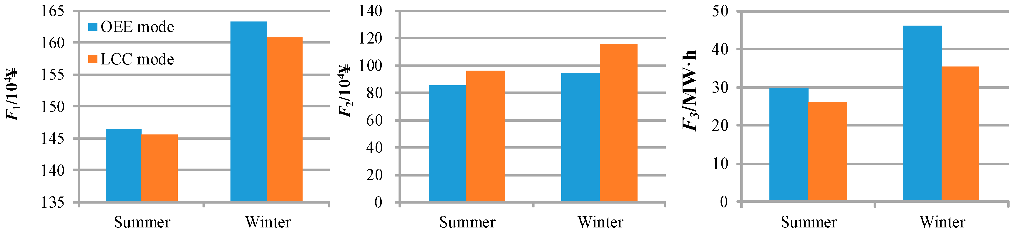
6.3. Results Analysis

The above analysis has already demonstrated the influences of different ESD modes on MECS operation. To prove the optimization effect of the ESD on MECS operation, the MECS was scheduled without the ESD to comparatively analyze the results of different operation scenarios. The comparative analysis index encompassed the objective function values, the pollutant emissions, the complementarity indexes, and the load demand curve.

Table 5. The comparative results of MECS scheduling under different operation scenarios.

Scene		Objective Function			Pollutant Emissions/Tonne			Complementarity Indexes			Load Demand/MW
		F1/104 ¥	F2/104 ¥	F3/MW	CO2	SO2	NOx	LTD/%	SPC/MW·h	Coal Consumption/(g/kW·h)	Peak	Valley
OEE mode	Summer	146.49	85.83	29.67	3794	92	87	57	33.64	310.05	1795	1485
	Winter	163.22	94.34	46.33	3883	94	90	32	44.12	312.60	1765	1415
LLC mode	Summer	145.65	95.84	26.33	4158	101	95	52	26.86	315.91	1808	1450
	Winter	160.85	115.62	35.33	4233	103	97	40	34.22	316.85	1788	1408
Without ESD	Summer	142.18	115.54	30.15	4181	101	96	48	18.59	324.80	1820	1430
	Winter	158.45	128.29	36.85	4381	106	101	30	26.17	329.90	1794	1398

shows the comparative results of MECS scheduling under different operation scenarios.

When the MECS was scheduled without the ESD, the values of all objective functions worsened. For example, in the LLC mode, the value of F₁ decreased by 43.1 thousand ¥ on a typical summer day, and by 47.7 thousand ¥ on a typical winter day, compared with the corresponding values in the OEE mode. In the OEE mode, the value of F₃ increased by 3.78 MW on a typical summer day and by 1.52 MW on a typical winter day, compared with the corresponding values in the LLC mode. The outputs of WPP and PV decreased without ESD, as the load demand had to be partly satisfied by thermal power units. Therefore, pollution emissions increased significantly. For example, the total CO₂ emission increased by 378 tons and by 189 tons on two typical days, compared with the values in the LLC mode. Consequently, the values of the complementarity indexes also worsened. The LTD reached its lowest value, i.e., 30%, and the SPC and UCC reached their highest values, i.e., 26.17 MW·h and 329.9 g/kW·h. Figure 13 shows the scheduling results of the MECS operation without the ESD on a typical day.

According to Figure 13, when ESD was not considered, TPP4 was used to provide a reserve service on a typical summer day and part-time service on a typical winter day. TPP3 was also scheduled for full-time load demand satisfaction, and part-time reserve service. For example, TPP3 was scheduled with a power output of 199 MW·h from 3:00 h to 5:00 h as a reserve service. Moreover, the abandoned power outputs of WPP and PV were 1123.8 MW·h and 412.35 MW·h, respectively, on a typical summer day and 2005.35 MW·h and 340.65 MW·h on a typical winter day. Thus, the total power generation cost reached 6148.47 tce and 6442.46 tce on the two typical days, respectively. Obviously, the power output structure without the ESD was worse than that with the ESD. Figure 14 shows the net output curve of the thermal power units under different operational strategies.

It can be seen that as the ESD charges when load demand is low and discharges when load demand is high, the load demand curve is smoother. Combined with Table 5, if the ESD is not considered, the peak–valley ratio of the net load demand (thermal power out) curve reached the highest value of 2.24 on a typical summer day, and 1.37 on a typical winter day. However, the corresponding ratios in the OEE mode were 1.75 and 1.26, and 1.95 and 1.31 in the LLC mode. Overall, to smooth the load demand curve to improve the space of WPP and PV, ESD should be integrated into the MECS.

To analyze the influence of the capacity of the ESD on MECS operation, a sensitivity analysis of the ESD capacity was carried out. The values of the objective functions and the complementarity indexes were calculated for different ESD capacities. Assuming that the maximum and rated discharge–charge power of the ESD are positively correlated with the ESD capacity, the optimal MECS operation can be obtained for different ESD capacities. Figure 15 shows the objective function value of the MECS operation with different ESD capacities.

It can be seen that when the MECS was scheduled on a typical summer day, the ESD capacity demand for MECS operation was low, as the available WPP output was relatively low. When the ESD capacity reached 1000 MW in the OEE mode, the values of objective functions reached the limit values, namely, F₁, F₂, and F₃ were equal to 1553.8 thousand Yuan, 708.2 thousand Yuan, and 24.32 MW, respectively. The values of the objective functions were nearly unchanged when the capacity was more than 1000 MW, namely, the capacity ratios of the ESD to the WPP and the ESD to the PV reached 0.77. The ratio was 1.08 in the LLC mode.

However, when the ESD was scheduled on a typical winter day, the ESD capacity demand for the MECS operation was relatively high as the available WPP output was high. When the ESD capacity reached 1400 MW in the OEE mode, the values of the objective functions reached the same limit values as on a typical summer day. Thus, the corresponding ratios were 0.92 and 1.23. Overall, the values of the objective functions were better when the ESD capacity was high. However, they reached the limit values when the ESD capacity reached the required capacity. Figure 16 shows the values of the complementarity indexes under different ESD capacities.

It can be seen that the values of the complementarity indexes improved as the ESD capacity increased. It should be noted that this trend was not always continuous. When the MECS was scheduled on a typical summer day, the change was small once the ESD capacity reached 800 MW in the OEE mode and 1300 MW in the LLC mode, i.e., the capacity ratios of the ESD to the WPP and the ESD to the PV were 0.62 and 1, respectively. However, when the MECS was scheduled on a typical winter day, the change was small once the ESD capacity reached 1300 MW in the OEE mode and 1700 MW in the LLC mode, i.e., the capacity ratios of the ESD to the WPP and the ESD to the PV were 1 and 1.31, respectively. Overall, the change trend of the complementarity indexes was nearly identical to that of the objective functions. When the capacity ratios of the ESD to the WPP and the ESD to the PV belonged to [0.62, 0.77] in the OEE mode and [1, 1.08] in the LLC mode, the optimal results of MECS scheduling were obtained on a typical summer day, whereas for capacity ratios in [0.92, 1] in the OEE mode and [1.23, 1.31] in the LLC mode, the optimal results were obtained on a typical winter day. Therefore, the optimal ESD capacity and operation strategy for MECS operation should be determined according to the actual operating environment.

7. Conclusions

WPPs, PVs, HSs, TPPs, and ESDs were integrated into a MECS. This paper proposed a multi-objective model for MECS operation considering different operation constraint conditions under three objective functions: the maximum operation revenue (F₁), the minimum abandoned energy cost (F₂), and the minimum output fluctuation (F₃). Then, the rough set theory was applied to handle the information of the payoff table of the objective functions to calculate the weight coefficients. Finally, the improved IEEE 14-bus system was used as the simulation system. The following conclusions were gained:

(1) The proposed uncertainty analysis and simulation method generated the most appropriate scenarios for wind power, photovoltaic power, and other uncertainty factors. The Wasserstein method achieved a better discretization by dividing the CPDF into several unequal subintervals. The scenario tree method comprehensively simulated the uncertainty factors by considering different occurrence states, whereas the improved K-medoids method selected the most representative scenarios more efficiently by calculating the relative K-distances of different scenarios and ensuring the updated clustering center.

(2) The MECS fully utilized the complementarity of the different power sources, and the proposed multi-objective model obtained the optimal scheme for MECS scheduling. TPPs, HSs, and PVs were the major power sources used to satisfy the load demand on a typical summer day, whereas TPPs and WPPs were the major power sources used for load demand on a typical winter day. Compared with the results of the single optimization objective, the scheduling results better balanced the revenue and risk when multiple optimization objectives were taken into consideration.

(3) The operation results of MECS scheduling improved as the ESD capacity increased, and they were restricted when the capacity reached the required value. The change trend of the complementarity indexes was nearly identical to that of the objective functions. The ESD optimized the MECS scheduling by utilizing the characteristics of power discharge–charge. The ESD operation mode directly influenced the optimality of the results. In the OEE mode, the discharge–charge power was better utilized than in the LLC mode; moreover, the LLC mode ensured the ESD’s operation life cycle. The optimal ESD operation strategy should be individually determined to achieve the optimal scheme for MECS operation.

(4) The operation results of MECS scheduling improved as the ESD capacity increased, and they were restricted when the capacity reached the required value. The change trend of the complementarity indexes was nearly identical to the objective functions. When the capacity ratios of the ESD and the WPP and the PV was in [0.62, 0.77] in the OEE mode and in [1, 1.08] in the LCC mode, the optimal results of MECS scheduling were obtained on a typical summer day. When the capacity ratios were in [0.92, 1] in the OEE mode and in [1.23, 1.31] in the LCC mode, the optimal results were obtained on a typical winter day. The optimal ESD operation strategy should be individually determined.

References

1. Zhang, Q.X.; Liao, H.; Hao, Y. Does one path fit all? An empirical study on the relationship between energy consumption and economic development for individual Chinese provinces. Energy 2018, 150, 527–543. [Google Scholar] [CrossRef]
2. Liu, H.L.; Andresen, G.B.; Greiner, M. Cost-optimal design of a simplified highly renewable Chinese electricity network. Energy 2018, 147, 534–546. [Google Scholar] [CrossRef] [Green Version]
3. Mu, Y.Q.; Cai, W.J.; Evans, S.; Wang, C.; David, R.-H. Employment impacts of renewable energy policies in China: A decomposition analysis based on a CGE modeling framework. Appl. Energy 2018, 210, 256–267. [Google Scholar] [CrossRef]
4. Song, D.; Keith, W.H.; Dang, Y.G. Forecasting China’s electricity consumption using a new grey prediction model. Energy 2018, 149, 314–328. [Google Scholar]
5. Song, J.J.; Wang, J.Z.; Lu, H.Y. A novel combined model based on advanced optimization algorithm forshort-term wind speed forecasting. Appl. Energy 2018, 215, 643–658. [Google Scholar] [CrossRef]
6. Mojtaba, D.; Mustafa, J.R.; Ahmad, Z.C. Short-term power output forecasting of hourly operation in power plant based on climate factors and effects of wind direction and wind speed. Energy 2018, 148, 775–788. [Google Scholar]
7. Shaikh, M.R.; Randall, S.; Erik, H.; Grant, A.K. The levelized costs of electricity generation by the CDM power projects. Energy 2018, 148, 235–246. [Google Scholar]
8. Kim, J.W.; Noh, Y.L.; Chang, D.J. Storage system for distributed-energy generation using liquid air combined with liquefied natural gas. Appl. Energy 2018, 212, 1417–1432. [Google Scholar] [CrossRef]
9. Atherton, J.; Sharma, R.; Salgado, J. Techno-economic analysis of energy storage systems for application in wind farms. Energy 2017, 135, 540–552. [Google Scholar] [CrossRef]
10. Tan, Z.F.; Wang, G.; Ju, L.W.; Tan, Q.K.; Yang, W.H. Application of CVaR risk aversion approach in the dynamical scheduling optimization model for virtual power plant connected with wind-photovoltaic-energy storage system with uncertainties and demand response. Energy 2017, 124, 198–213. [Google Scholar] [CrossRef]
11. Morteza, S.; Mohammad-Kazem, S.E.E.; Mahmoud-Reza, H. An interactive cooperation model for neighboring virtual power plants. Appl. Energy 2017, 200, 273–289. [Google Scholar]
12. Derrouazin, A.; Aillerie, M.; Mekkakia-Maaza, N.; Charles, J.P. Multi input-output fuzzy logic smart controller for a residential hybrid solar-wind-storage energy system. Energy Convers. Manag. 2017, 148, 238–250. [Google Scholar] [CrossRef]
13. Zhang, H.F.; Yue, D.; Xie, X.P.; Dou, C.X.; Sun, F. Gradient decent based multi-objective cultural differential evolution for short-term hydrothermal optimal scheduling of economic emission with integrating wind power and photovoltaic power. Energy 2017, 122, 748–766. [Google Scholar] [CrossRef]
14. Hassan, F. Novel standalone hybrid solar/wind/fuel cell power generation system for remote areas. Sol. Energy 2017, 146, 30–43. [Google Scholar]
15. Mason, I.G. Comparative impacts of wind and photovoltaic generation on energy storage for small islanded electricity systems. Renew. Energy 2015, 80, 793–805. [Google Scholar] [CrossRef]
16. Ghada, B.; Lotfi, K. A dynamic power management strategy of a grid connected hybrid generation system using wind, photovoltaic and Flywheel Energy Storage System in residential applications. Energy 2014, 71, 148–159. [Google Scholar]
17. Iman, G.M.; Mostafa, N.; Farhad, F.; Mohsen, S.; Saeid, M. Risk-averse profit-based optimal operation strategy of a combined wind farm–cascade hydro system in an electricity market. Renew. Energy 2013, 55, 252–259. [Google Scholar]
18. Okan, A.; Oya, E.K. Cost and emission impacts of virtual power plant formation in plug-in hybrid electric vehicle penetrated networks. Energy 2013, 60, 116–124. [Google Scholar] [Green Version]
19. Kaabeche, A.; Belhamel, M.; Ibtiouen, R. Sizing optimization of grid-independent hybrid photovoltaic/wind power generation system. Energy 2011, 36, 1214–1222. [Google Scholar] [CrossRef]
20. Aboelsood, Z.; Hossam, A.G.; Ahmed, E. Optimal planning of combined heat and power systems within microgrids. Energy 2015, 93 Pt 1, 235–244. [Google Scholar]
21. Heidelberger, P.; Norton, A.; Robinson, J.T. Parallel quicksort using fetch-and-add. IEEE Trans. Comput. 1990, 39, 133–138. [Google Scholar] [CrossRef]
22. Fu, X.Q.; Guo, Q.L.; Sun, H.B.; Pan, Z.; Xiong, W.; Wang, L. Typical scenario set generation algorithm for an integrated energy system based on the Wasserstein distance metric. Energy 2017, 135, 153–170. [Google Scholar] [CrossRef]
23. Al-Shammari, E.T.; Shamshirband, S.; Petković, D.; Zalnezhad, E.; Yee, P.L.; Taher, R.S.; Ćojbašić, Ž. Comparative study of clustering methods for wake effect analysis in wind farm. Energy 2016, 95, 573–579. [Google Scholar] [CrossRef]
24. Wang, Q.; Dong, W.L.; Yang, L. A wind power/photovoltaic typical scenario set generation algorithm based on wasserstein distance metric and revised K-medoids cluster. Proc. CSEE 2015, 35, 2654–2661. [Google Scholar]
25. Ju, L.W.; Tan, Z.F.; Li, H.H.; Tan, Q.K.; Yu, X.B.; Song, X.H. Multi-objective operation optimization and evaluation model for CCHP and renewable energy based hybrid energy system driven by distributed energy resources in China. Energy 2016, 111, 322–340. [Google Scholar] [CrossRef]
26. Deng, C.; Ju, L.W.; Liu, J.Y.; Tan, Z.F. Stochastic Scheduling Multi-Objective Optimization Model for Hydro-Thermal Power Systems Based on Fuzzy CVaR Theory. Power Syst. Technol. 2016, 40, 1447–1457. [Google Scholar]
27. Liu, G.L. Rough set theory based on two universal sets and its applications. Knowl.-Based Syst. 2010, 23, 110–115. [Google Scholar] [CrossRef]
28. Adhvaryyu, P.K.; Chattopadhyay, P.K.; Bhattacharya, A. Dynamic optimal power flow of combined heat and power system with Valve-point effect using Krill Herd algorithm. Energy 2017, 127, 756–767. [Google Scholar] [CrossRef]
29. Available online: http://www.tanpaifang.com/tanzhibiao/201601/2350250.html (accessed on 27 February 2016).
Figure 1. The basic structure of the multi-energy complementary system (MECS) operation.
Applsci 08 02293 g001
Figure 2. The discretization of the continuous probability distribution functions (CPDFs) (six discrete points).
Applsci 08 02293 g002
Figure 3. The uncertainty simulation flowchart. PV: photovoltaic power plant; WPP: wind power plant.
Applsci 08 02293 g003
Figure 4. The load demand and the available output of the hydropower station (HS) on a typical load day.
Applsci 08 02293 g004
Figure 5. The ten simulation scenarios of WPPs and PVs on a typical load day (summer).
Applsci 08 02293 g005
Figure 6. The average outputs of WPP and PV on a typical load day (summer and winter).
Applsci 08 02293 g006
Figure 7. The optimization flowchart for the MECS scheduling model.
Applsci 08 02293 g007
Figure 8. The different objective values under the comprehensive objective function on typical days.
Applsci 08 02293 g008
Figure 9. The MECS scheduling results on typical days under the OEE mode: summer (left) and winter (right).
Applsci 08 02293 g009
Figure 10. The MECS scheduling results on a typical day under the LLC mode: summer (left) and winter (right).
Applsci 08 02293 g010
Figure 11. The complementarity indexes of MECS operation under different energy storage devices (ESD) operation modes.
Applsci 08 02293 g011
Figure 12. The power output structure of MECS scheduling under the OEE mode: (a) summer and (b) winter.
Applsci 08 02293 g012
Figure 13. The scheduling results of the MECS operation without ESD on a typical day: (a) summer and (b) winter.
Applsci 08 02293 g013
Figure 14. The net output curve of the thermal power units under different operational strategies.
Applsci 08 02293 g014
Figure 15. The objective function values of MECS operation under different ESD capacities.
Applsci 08 02293 g015
Figure 16. The complementarity indexes of MECS operation under different ESD capacities.
Applsci 08 02293 g016