Salt and Pepper Noise Removal for Image Using Adaptive Pulse-Coupled Neural Network Optimized by Grey Wolf Optimization and Bidimensional Empirical Mode Decomposition

Abstract

Aimed at the problem of poor noise reduction effect and parameter uncertainty of pulse-coupled neural network (PCNN), a hybrid image denoising method, using an adaptive PCNN that has been optimized by grey wolf optimization (GWO) and bidimensional empirical mode decomposition (BEMD), is presented. The BEMD is used to decompose the original image into multilayer image components. After a GWO is run to complete PCNN parameter optimization, an adaptive PCNN filter method is used to remediate the polluted noise points that correspond to the different image components, from which a reconstruction of the denoised image components can then be obtained. From an analysis of the image denoising results, the main advantages of the proposed method are as follows: (i) the method effectively solves the deficiencies that arise from the critical PCNN parameter determination issue; (ii) the method effectively overcomes the problem of high-intensity noise effects by providing a more targeted and efficient noise reduction process; (iii) when using this method, the noise points are isolated, and the original pixel points are restored well, which can lead to preservation of image detail information. When compared with traditional image denoising process algorithms, the proposed method can yield a better noise suppression effect, based on indicators including analysis of mutual information (MI), structural similarity (SSIM), the peak signal-to-noise ratio (PSNR) and the standard deviation (STD). The feasibility and applicability of the proposed denoising algorithm are also demonstrated experimentally.

1. Introduction

The recent boom in the development of digital technology and multimedia communications has seen digital image analysis methods for nonlinear and nonstationary data receive widespread attention. In digital image processing and analysis in particular, image noise is an important research topic for many different application fields, such as image transmission, image matching, target detection, and remote sensing. However, a wide variety of interference types can disrupt the analysis process. In interference preclusion processes, the existence of noise inevitably leads to image quality degradation, which results in blurring and distortion of valid pixels. Therefore, for digital images, the visual pixel quality must be guaranteed using reliable and effective approaches. Consequently, noise reduction measures are indispensable to maintaining high recognition accuracy and preserving valid pixels for image analysis [1,2]. To review the existing research works, based on sparse and redundant representations over trained dictionaries, the Bayesian treatment applying K-SVD can yield a state-of-the-art denoising performance [3]. As the digital implementation of new mathematical transformation, the curvelet transform can outperform wavelet methods in image denoising and certain image reconstruction problems [4]. The sparse 3-D transform-domain collaborative filtering can yield a satisfying image denoising effect as a novel image strategy [5]. Block matching 3D denoising (BM3D) is an excellent single-image denoising method [6], and BM3D is a well-engineered algorithm which can achieve the state-of-the-art denoising performance with a plain multi-layer perceptron (MLP) [7]. The pulse-coupled neural network (PCNN) has been studied very extensively. As an effective nonlinear digital data analysis method, it is well capable of isolating noisy pixel points and eliminating high-intensity noise during image processing [8]. In this paper, we are committed to the study of noise reduction effect of PCNN and make improvements to the PCNN method.

Initially inspired by the visual cortexes of cats, the PCNN was progressively developed based on synchronous dynamic neuronal activity [9]. From analysis of the acting mechanism, PCNNs actually have the functional characteristics of neuron-specific linear addition, bioelectric pulse transmission through ion channels, nonlinear modulation, and synchronous pulse release [10]. In current digital image processing, PCNNs can be applied to many aspects, including image fusion, image segmentation, and feature extraction. Xie et al. [11] applied a memristor-based circuit implementation of a PCNN with dynamic threshold generators in the digital image processing field. Ding et al. [12] combined a PCNN with the nonsubsampled contourlet (NSCT) model to overcome the coefficients selection problem for the NSCT sub-band that provided an innovative image fusion method based on an image gradient motivation. Yang et al. [13] presented a multifocus image fusion method that was based on robust sparse representation (RSR) and an adaptive PCNN.

Many researchers have also conducted relevant studies on image denoising. Deng et al. [14] introduced an adaptive denoising multilayered PCNN for application to salt and pepper noise removal. Zhu et al. [15] researched a memristive PCNN (M-PCNN) for medical image denoising processes, which makes the network have a biological function. Bai et al. [16] applied particle swarm optimization (PSO) to the implementation of PCNN parameter optimization. Shen et al. [17,18] proposed an innovative genetic ant colony algorithm (GACA)-based combination with the PCNN approach to accomplish good quality image denoising. As a preprocessing digital image noise reduction method, the PCNN has several issues that must be resolved to achieve better results. The PCNN is a complex model system that included an input system and a feedback system. In many cases, the predefined network parameters mean that the researchers must try to select suitable parameters, many times, contemporaneously, in response to different input images. To address the above issues, many methods, including simplified models and intelligent swarm models, are used to improve the image denoising performance. Wu et al. [19] proposed a simplified PCNN method with adaptive parameters that was excellent in terms of both visual appearance and parameter setting. He et al. [20] applied a cuckoo search (CS) algorithm based on a simple PCNN model to a multi-parameter optimization problem. Xu et al. [21] introduced a quantum-behaved particle swarm optimization (QPSO) model to optimize the PCNN model with good effect.

It should be pointed out that the existing related optimization algorithms that are introduced for setting PCNN parameters have several common disadvantages that must be resolved, including complex search mechanisms, easy relapse into local optimum behavior, and low generalization capabilities. In addition, the fitness functions of these optimization methods must be modified to promote both search efficiency and generalization ability. A fast and accurate parameter optimization is a hot issue that needs to be resolved in PCNN, which is also a major content of this paper. Moreover, analysis of whole image denoising processes shows that the optimized PCNN combined with filtering can produce a particular noise reduction effect. However, when faced with high-intensity noise, the entire noise reduction process becomes challenging [22]. Some of the noise will always be left over and will affect image clarity and detail recognition. Furthermore, in the current situation, most noise suppression methods that play a good role in low intensity noise include conventional filters such as a single median filter. How to settle the contaminated complicated characteristics and incomplete noise suppression puzzles caused by high-intensity noise are hot spot research topics. Additionally, in the field of image noise reduction, how to keep as much image detail as possible and restore the original image information for use, are also major problems.

Motivated by the above analysis, we focus on the improvement of the noise reduction effect of PCNN images denoising. To overcome the limitation of the existing PCNN parameter optimization problem and meet better noise reduction requirements, an adaptive PCNN model in which the PCNN parameters are optimized using the grey wolf optimization (GWO) algorithm to address the parameter issues described above. As a meta-heuristic optimization technique, the GWO has merits that include simplicity, flexibility, a derivation-free mechanism, and avoidance of local optima [23]. Under its leadership hierarchy and hunting mechanism, the GWO is capable of filtering, completing iteration and optimization of a series of parameters [24]. At the same time, the GWO provides high convergence speeds and high optimization accuracy. After the Experiments, GWO is applicable to challenging problems with unknown search spaces [25]. Furthermore, for high-intensity noise suppression, further research about bidimensional empirical mode decomposition (BEMD) is introduced in an innovative way. BEMD is actually very widely used in image processing, such as image denoising, and is an extension of Huang’s empirical mode decomposition (EMD) method [26]. The high-intensity contaminated noise will be very concentrated and dense in the polluted image. BEMD is applied to decompose the heavily contaminated image into several bidimensional intrinsic mode functions (BIMFs). In this way, high-intensity noise can be dispersed into smaller components, and use of the BEMD effectively accomplishes an image-adapted decomposition procedure to provide image-noise separation. The decomposed image components are then more compatible with the processing conditions required for the optimized PCNN method. In fact, there are many denoising algorithms that are two steps and similar to the PCNN method, where the first step isolates noisy pixels and the second one suppresses the noise. For example, Salim [27] introduced a non-linear complex diffusion process (NLCDP) technique in the tBEMD domains, where the tBEMD is an adjusted BEMD method built on Student’s probability density function (PDF). The tBEMD-NLCDP method has an advantage over the traditional BEMD method. The main contributions in this paper are summarized as follows.

Committed to PCNN image noise reduction research, an adaptive PCNN method that is combined with the GWO and BEMD algorithms is developed, which has significant benefits for use in image denoising. But its parameters are difficult to determine which limits its practical application. GWO algorithm is firstly proposed to resolve PCNN parameter issues, which can adaptively optimize parameters exactly, with a global optimal solution and rapid convergence. Through a process of continuous hierarchy screening and multiple iterations, the optimized parameters can have high accuracy via the experimental verification and will enhance the PCNN’s denoising performance well. The PCNN application isolates the noisy pixels and the noise-polluted image can be processed more easily. Therefore, a subsequent filter, such as a median filter, can yield better denoising results. Importantly, BEMD will be applied to decompose the raw heavily polluted image into different components. This step is significant, solving the problem of a one-time direct processing, which makes it difficult to reduce the high-intensity image noise thoroughly. The decomposed high and low-frequency components are then denoised using the optimized PCNN filter method. For important novelties, the GWO intelligent algorithm is the first proposed to apply intelligent optimization screening to parameters, which solves the key parameter problem accurately. BEMD application makes the denoising progress more targeted according to the different component conditions. The self-adaptive determination optimized PCNN parameters will make the noise suppression progress fascinating while it is assisted.

The proposed BEMD-GWO-PCNN denoising method is mainly applied to complete offline image processing. The method effectively improves the effectiveness of parameter optimization and greatly accelerates the parameter optimization operating speed. Application of BEMD remedies the previous deficiencies of insufficient suppression of high-intensity noise by making the denoising process more specific. The image reconstruction results can finish excellent extraction, preservation of image details, and good noise suppression performance. In this paper, the existing other PCNN based noise reduction methods are compared with our proposed method. In terms of parameter optimization efficiency and actual noise reduction effects, the proposed method applied to image denoising is superior. According to our evaluation indicators, the proposed BEMD-GWO-PCNN method is shown to be feasible and to be more accurate than other conventional and PCNN-based denoising methods.

The article is organized as follows: Section 2 is the description of adaptive PCNN combined with GWO and BEMD; Section 3 is the experimental results and analysis; And the last section provides conclusions and challenges for future research.

2. Adaptive PCNN Combined with GWO and BEMD

2.1. Introduction of Intrinsic Mode Functions

Unlike the traditional integral transform techniques, EMD is a multi-scale partial wave analysis method. However, BEMD offers higher frequency resolution and more accurate timing of nonlinear and nonstationary signal events. After a sifting process is applied to the input signal, the intrinsic mode functions (IMFs) can be obtained. The IMF components can be defined using two conditions: (1) the number of extrema and the number of zero-crossings should either be equal or differ only by no more than one; (2) at each point, the mean of the defined envelope through the local maxima and the envelope that is defined by the local minima must be zero. Then, the decomposed result of the IMFs denoted by $m_i$ and the residue rare as shown:

$$s={\displaystyle \sum _{i=1}^n{m}_i}+r$$

(1)

where s is defined as the input signal, n demonstrates the number of the IMFs.

The IMF components represent each of the frequencies of the local data and thus correspond to both high-frequency and low-frequency data. The residue function component represents the tendency of the original image. The exact results of the IMFs constitute the BEMD [28].

2.2. Theories of the BEMD

As a data driven method, the BEMD is developed based on envelope analysis and a sifting process, and can decompose complex signals into a number of components that have the local characteristics of the input source image [29]. The number of BIMFs is determined by the image data itself, where different images correspond to different numbers of BIMFs after decomposition. A BIMF must meet two constraints: (1) the local mean of the original bidimensional signals must be symmetrical and the mean is zero; and (2) the maximum of the BIMF is positive, while the minimum is negative [30].

The local BIMF frequencies range from high to low order when they are extracted layer-by-layer. The image signal energy is mainly concentrated in the low-frequency region; in contrast, the interfering noise is mostly located in the high-frequency region. The local BIMF frequencies include strong physical contrast information, including highlight edges of the source images, and the line and zone boundaries [31]. Each BIMF component contains different frequency coefficients, and the high—frequency coefficients are in a lower order. The residue function image contains the low-frequency information of the source image, for which the grey-level distribution and the gradient information are smooth. The BEMD method can then effectively extract the various details and edges of the source image. From the perspective of the primary function, the BEMD can generate different primary functions $g_i$ adaptively, corresponding to different source image characteristics. BEMD differs from Fourier transforms and wavelet decomposition, which have functions $g_{is}$ that are predetermined [32]. In this work, we have adapted BEMD to decompose a raw image into several BIMFs and residue images through an interpolation and envelope operation. The image BEMD decomposition result $f(x_1,y_1)$ of $u\times v$ neighboring pixels is as shown below:

$$f(x_1,y_1)={\displaystyle \sum _{l=1}^v{c}_l(x_1,y_1)}+r_v(x_1,y_1)$$

(2)

where $c_l(x_1,y_1)$ represents the decomposed l-th components, and $r_v(x_1,y_1)$ is the residue or trend term. The basic decomposition process steps of BEMD are as follows:

(a)

Initialize the raw image and set the pending image $f(x_2,y_2)$, where $r_l(x_2,y_2)=f(x_2,y_2)$.

(b)

If z = 1, set $h_{lz}\left(x_2,y_2\right)=r_l\left(x_2,y_2\right)$; otherwise, set $h_{l+1}(x_2,y_2)=r_l$, and $l=l+1$.

(c)

Calculate the maximum spectrum value $p_{lz}$ and the minimum spectrum values $q_{lz}$ corresponding to $v_{lz}(x_2,y_2)$.

(d)

Interpolate the calculated maximum spectrum $p_{lz}$ and the minimum spectrum values $q_{lz}$ draw the upper envelope $u_{max}(x_2,y_2)$ of $h_{lz}\left(x_2,y_2\right)$, and draw the lower envelop $n_{min}\left(x_2{y}_2\right)$ of $h_{lz}\left(x_2,y_2\right)$.

(e)

Calculate the mean envelope $v_{lz}(x_2,y_2)$ of $h_{lz}(x_2,y_2)$ using the following formula:

$$v_{lz}(x_2,y_2)=\frac{u_{max}(x_2,y_2)+n_{min}(x_2,y_2)}{2}$$

(3)

(f)

Set $h_{l(z+1)}(x_2,y_2)$ to be the partial information of the source image, which can be calculated using (4):

$$h_{l\left(z+1\right)}\left(x_2,y_2\right)=h_{lz}\left(x_2,y_2\right)-v_{lz}\left(x_2,y_2\right)$$

(4)

(g)

Check whether the characteristics of $h_{l(z+1)}(x_2,y_2)$ satisfy the BIMF properties; use the standard deviation (STD) between $h_{z+1}$ and $h_z$ as the stopping criterion from (5). It can be used to determine whether $h_{l(z+1)}(x_2,y_2)$ meets the BIMF characteristics from two consecutive sifting results. Limitation of the size of the STD allows a criterion for stopping of the sifting process to be determined. From prior experience, the STD value can generally be set in the 0.2–0.3 range.

$$SD=\frac{{{\displaystyle {\sum }_{x_2=1}^u{\displaystyle {\sum }_{y_2=1}^v\left|h_{l\left(z+1\right)}\left(x_2,y_2\right)-h_{lz}\left(x_2,y_2\right)\right|}}}^2}{{\displaystyle {\sum }_{x_2=1}^u{\displaystyle {\sum }_{y_2=1}^v\left|h_{lz}\left(x_2,y_2\right)\right|}}}$$

(5)

(h)

If the STD is less than a specified threshold and $h_{l(z+1)}(x_2,y_2)$ does not meet the stop condition, then set $l=l+1$ and return to step c) until the sifting process condition is met. If $h_{l(z+1)}(x_2,y_2)$ reaches the stop condition, then $c_l\left(x_2,y_2\right)=h_{l\left(z+1\right)}\left(x_2,y_2\right)$ and $r_{l+1}=r_l-h_l(x_2,y_2)$; $l=l+1$.

Initially, the decomposition performs a preliminary pre-denoising treatment of the composite image signal. The decomposed components are specific to a single spectral component that has stabilized features and lower disturbances. The decomposition result enables reduction of the complexity of image analysis with heavy noise. Therefore, the application of BEMD primarily ensures the accuracy of the analysis with the illusion of heavy noise elimination. BEMD thus appears to be an impressive option for achieving more practical noise reduction in the final processed image.

2.3. Implementing the PCNN Theory

Eckhorn [33] proposed the pulse-coupled neural network, which is a third-generation artificial neural network with wide application potential. In 1999, Johnson [34] used circuit theory to introduce the PCNN model more specifically, which was subsequently widely applied in various image processing fields. Today, the continuous development of the PCNN model has given it incomparable superiority over the other current image denoising methods. There are two notable features of PCNN in the form of the global coupling and pulsed synchronization of the neurons [35]. In image processing, a PCNN is a single layer two-dimensional array of laterally linked neurons. Each neuron in the network corresponds strictly to one pixel only in an input image and receives the intensity of that corresponding pixel as an external stimulus. Each neuron also connects with its neighboring neurons and receives local stimuli from them. The PCNN model (Figure 1) is composed of three parts: the dendritic tree of the coupled linking subsystem, the modulation subsystem, and the pulse generator of the dynamic threshold subsystem and the firing subsystem.

The surrounding outputs of the PCNN in the last iteration can be obtained using the linking compartment, while the initial output of the PCNN is set to zero [36]. For the input stimulus, the feeding compartment is applied at the corresponding location. Overall, the dendritic tree is defined mathematically as shown below:

$$F_{ij}\left[c\right]=I_{ij}$$

(6)

$$L_{ij}\left[c\right]=V_L{\displaystyle \sum _{k,l}{W}_{ijkl}}Y\left[c-1\right]$$

(7)

where $F_{ij}\left[c\right]$ represents the feeding input compartment of neuron $\left(i,j\right)$ and $L_{ij}\left[c\right]$ is the linking compartment. $I_{ij}$ is the external stimulus of neuron $\left(i,j\right)$ and $V_L$ is a normalizing constant. $w_{ijkl}$ denotes the weighted coefficient of neurons $\left(k,l\right)$ to $\left(i,j\right)$, which is the reciprocal of the Euclidean distance and is defined as shown in (8) [9]:

$$W_{ijkl}=\frac{1}{\sqrt{{\left(i-k\right)}^2+{\left(k-l\right)}^2}}$$

(8)

The stimuli from the dendritic tree are applied to the modulation subsystem, and the modulation process can be described as shown in (9) below.

$$u_{ij}\left[c\right]=F_{ij}\left[c\right]\left\{1+{\beta }_T{L}_{ij}\left[c\right]\right\}$$

(9)

where ${\beta }_T$ is the linking strength factor between synapses, and $u_{ij}\left[c\right]$ denotes the internal state of the neuron.

Next, the threshold $E_{ij}\left[c\right]$, which represents the dynamical threshold, is generally set to zero. In each iteration, the threshold $E_{ij}\left[c\right]$ will be shown as follows:

$$E_{ij}\left[c\right]=e^{-{\alpha }^T}{E}_{ij}\left[c-1\right]+V_T{Y}_{ij}\left[c\right]$$

(10)

where ${\alpha }_T$ is the exponential decay time constant, and ${\nu }_T$ is the intrinsic voltage constant of $E_{ij}\left[c\right]$.

Finally, the internal state $U_{ij}\left[c\right]$ must be compared with that of the dynamic threshold $E_{ij}\left[c\right]$, and the pulse output $Y_{ij}\left[c\right]$ can be obtained subsequently using the firming subsystem:

$$Y_{ij}\left[c\right]=\{\begin{array}{l}1,U_{ij}\left(c\right)>E\left[c-1\right],\\ 0,U_{ij}\left(c\right)\le E\left[c-1\right],\end{array}$$

(11)

The neuron’s pulse generator includes a step function generator and a threshold signal generator. The threshold input at each time step is updated using the form of an exponential decay. At each step, the neuron output $Y_{ij}\left[c\right]$ is set as 1, which means it can be fired. The internal activity $U_{ij}\left[c\right]$ is greater than the threshold function $E_{ij}\left[c\right]$. The neuron output $Y_{ij}\left[c\right]$ is then reset to zero when $U_{ij}\left[c\right]$ is less than $E_{ij}\left[c\right]$. Thus, in a single time step, the pulse generator produces a single pulse at its output whenever the values of $U_{ij}\left[c\right]$ exceed those of $E_{ij}\left[c\right]$.

The linking parameter ${\beta }_T$ is taken on as a global variable. ${\alpha }_T$ and ${\nu }_T$ are critical parameters that can easily affect the PCNN processing treatment. In this work, we initialize the weighted coefficient $W_{ijkl}$ as [0.707 1 0.707, 1 0 1, 0.707 1 0.707] based on prior work from the empirical selection [17], while the significant parameter optimization problem of ${\alpha }_T$, ${\beta }_T$ and ${\nu }_T$ of the PCNN when applied to image noise elimination is the ground-breaking core of this paper.

The PCNN has characteristics that include a capture feature and a synchronization release pulse, which are appropriate for image denoising, image segmentation and similar processes. In this paper, the high- and low-frequency domain images are denoised using the optimized PCNN methods. In allusion to heavy noise disturbance, the noise reduction mechanism of the PCNN is also introduced.

2.4. Noise Reduction Mechanism of PCNN

In the PCNN model, each neuron corresponds to a single image pixel, and the excitation of one neuron causes excitation of neighboring pixels with similar gray values; these responses are called synchronization release pulse characteristics [37]. Through application of these characteristics, a variety of the image processing methods mentioned above can be realized.

In this work, all of the neurons adopt the same connection behavior. The brightness information of every pixel will be input to the corresponding neurons. Every neuron will then be connected with the neurons in a $3\times 3$ neighboring region. The state of a neuron (i.e., firing or extinguishing) is dependent on the output of the firing system. The $F_{ij}\left[c\right]$ of every neuron corresponds to the highlight of the pixel points. $L_{ij}\left[c\right]$ is equal to the sum of the output responses from the $3\times 3$ neighboring neurons in channel L.

To overcome the noise disturbance and recover the detailed information as far as possible, noise elimination is necessary. By adjusting the brightness values of the image pixels, contaminated images can, to a certain extent, be recovered [38]. In most cases, the brightness values of the contaminated pixels differ from those of the neighboring normal pixels. Therefore, the outputs of noisy pixels differ from those of normal pixels. Based on the output states of each neuron and its neighboring neurons (i.e., ignited or unignited), the brightness values of the corresponding pixels are adjusted. The consequent improvement in the pixel values can eliminate the noise and promote detail preservation performance.

When the neuron output values are considered, the corresponding pixel brightness values will be declined when one neuron is ignited but most of its neighboring neurons are unignited; the corresponding pixel brightness values will increase when one neuron misfires, but most neighboring neurons do fire. In other cases, the brightness values will not change. Therefore, through application of the PCNN, the ignited matrix of the raw image can be obtained. From this perspective, the simplified PCNN model can locate the isolated noisy pixels accurately and suppress these isolated noisy pixel points. In the actual denoising process, the PCNN processing acts as the pre-processing procedure, and a filter operation is often used on the isolated pixels to achieve an improved noise reduction effect. In general, median filtering can be applied to the isolated points using the marked difference between the ignited pixels and the normal pixels. Many experiments have shown that the combination of the PCNN and a median filter is practical. A table showing the PCNN noise reduction algorithm with conventional random parameters (COR-PCNN; Algorithm 1) is introduced here in detail. From the model and the associated mechanism analysis, the parameters play a critical role in the PCNN treatment. In this study, we invested considerable effort in optimization of the critical parameters ${\alpha }_T$, ${\beta }_T$ and ${\nu }_T$, which performed well in our proposed GWO strategy.

Algorithm 1 PCNN Noise Reduction Algorithm

Boundary treatment: Generate edge-symmetric extension, make the original image (m, n) change into (m + 6, n + 6); Initialize the PCNN parameters: Initialize ${\alpha }_T$, ${\beta }_t$, ${\nu }_T$ and $W_{ijkl}$ the number of pass N, step length ${\Delta }_t$; Keep each pixel in an unignited condition; Contaminated points detection and treatment: Calculate every neuron $L_{ij}\left[c\right]$ values in $3\times 3$ neighboring region using Equation (7); adjust the threshold $L_{ij}\left[c\right]$ using Equation (10); calculate the neuron internal modulation signal $L_{ij}\left[c\right]$ using Equation (9); if a neuron (i, j) is ignited in $3\times 3$ neighbor region and more than 4 adjacent neurons are unignited, the (i, j) pixels brightness will decline an ${\Delta }_t$ end; if a neuron (i, j) is unignited in $3\times 3$ neighbor region and more than 4 adjacent neurons are ignited, the (i, j) pixels brightness will increase an ${\Delta }_t$ end; Otherwise the pixels brightness values of the (i, j) will not change end; Compare the $U_{ij}\left[c\right]$ e values and $E_{ij}\left[c\right]$ values, record the neuron output, ignited or unignited; $N=N-1$, if return to contaminated points detection and treatment end;

The time decay parameter α_T affects the operation efficiency directly and determines the number of iterations required in a cycle; V_T determines the conditions that must be issued only once in the iterative calculations. β_T has a major impact on restoration of the image. Therefore, we propose use of the GWO intelligent optimization algorithm to solve this complex nonlinear problem.

2.5. GWO Algorithm

Over recent decades, meta-heuristic optimization techniques, which are inspired by related physical phenomena, animal behavior or evolutionary concepts, have become increasingly popular [39]. Inspired by the behavior of grey wolves, the Grey Wolf Optimization (GWO) algorithm is a new meta-heuristics method. The tracking processes of grey wolves when encircling and attacking prey are the main steps in the numerical pattern of the GWO algorithm [40]. The GWO mimics the leadership hierarchy and the hunting mechanism of grey wolves in nature very well. The intelligent grey wolf optimizer was proposed by Mirjalili [41] and can perform appropriate trade-offs between the exploration and exploitation abilities of the algorithm. In solving complex benchmark functions, the GWO can be implemented effectively to address complex multivariate optimization problems. In the simulation of the leadership hierarchy, the grey wolves involve four types, designated α, β, δ and ω [42]. The hierarchy and relationships of the grey wolves and their corresponding duties are described in detail in Figure 2.

In the GWO, the optimal solution to the problem is considered to be the prey and first three best solutions are regarded as α, β and δ, respectively. Other than the three solutions mentioned above, ω must follow the three dominant wolves and holds the rest of the candidate solutions [43]. The initial stage of the GWO algorithm in the hunting process is encircling the prey. The mathematical formulation used to mimic the encircling process is given as follows:

$$\overrightarrow{D}=\left[\overrightarrow{C}\cdot {\overrightarrow{x}}_p\left(t\right)-\overrightarrow{x}\left(t\right)\right]$$

(12)

$$\overrightarrow{X}\left(t+1\right)={\overrightarrow{x}}_p\left(t\right)-\overrightarrow{A}\cdot \overrightarrow{D}$$

(13)

where t indicates the current iteration, ${\overrightarrow{x}}_p$ and $\overrightarrow{x}$ are the position vectors of the grey wolves and a grey wolf, respectively. The vectors $\overrightarrow{A}$ and $\overrightarrow{C}$ are calculated as follows:

$$\overrightarrow{A}=2\cdot \overrightarrow{a}\cdot {\overrightarrow{e}}_1-\overrightarrow{a}$$

(14)

$$\overrightarrow{C}=2\cdot {\overrightarrow{e}}_2$$

(15)

where ${\overrightarrow{e}}_1$ and ${\overrightarrow{e}}_2$ are random vectors in [0, 1], and $\overrightarrow{a}$ is a motion vector acting as a variable that decreases linearly from 2 to 0 over the iteration process. Depending on the random vectors ${\overrightarrow{e}}_1$ and ${\overrightarrow{e}}_2$ position updating can be performed randomly over the search domain.

We assume that α, β and δ all have better knowledge about the potential location of the prey. Therefore, the other grey wolves represented by ω are obliged to update their positions based on the best three positions obtained to date [44]. The grey hunting characteristic can then be presented numerically as follows:

$$\{\begin{array}{l}{\overrightarrow{D}}_a=\left|{\overrightarrow{C}}_1\cdot {\overrightarrow{X}}_a-\overrightarrow{X}\right|\\ {\overrightarrow{D}}_{\beta }=\left|{\overrightarrow{C}}_2\cdot {\overrightarrow{X}}_{\beta }-\overrightarrow{X}\right|\\ {\overrightarrow{D}}_{\delta }=\left|{\overrightarrow{C}}_3\cdot {\overrightarrow{X}}_{\delta }-\overrightarrow{X}\right|\end{array}$$

(16)

$$\{\begin{array}{l}{\overrightarrow{X}}_1={\overrightarrow{X}}_{\alpha }-{\overrightarrow{A}}_1\cdot {\overrightarrow{D}}_{\alpha }\\ {\overrightarrow{X}}_2={\overrightarrow{X}}_{\beta }-{\overrightarrow{A}}_2\cdot {\overrightarrow{D}}_{\beta }\\ {\overrightarrow{X}}_3={\overrightarrow{X}}_{\delta }-{\overrightarrow{A}}_3\cdot {\overrightarrow{D}}_{\delta }\end{array}$$

(17)

$$\overrightarrow{X}\left(t+1\right)=\frac{{\overrightarrow{X}}_1+{\overrightarrow{X}}_2+{\overrightarrow{X}}_3}{3}$$

(18)

The best three initial solutions are considered, and the residual solutions are eliminated, and thus the average measure of the three best solutions is provided by $\overrightarrow{X}$. The hunting process is terminated only after the prey is attacked and the prey should pause its movement. If $\overrightarrow{A}<1$, the attack process will be finished, but if $\overrightarrow{A}>1$, the grey wolves are diverted and move towards a better prey. Here, $\overrightarrow{a}$ represents the linear variable and the random vectors ${\overrightarrow{e}}_1$ and ${\overrightarrow{e}}_2$ are selected arbitrarily [45]. A table containing the GWO algorithm [41] is introduced in detail below (Algorithm 2).

Algorithm 2 Grey Wolf Optimization Algorithm

Initialize the grey wolf population number Yi (i = 1, 2, …, n) and max number of iterations N: Initialize random parameter vectors a, A, and C; Calculate the function fitness of each set of parameters $Y_a$ = the best search agent; $Y_{\beta }$ = the second-best search agent; $Y_{\delta }$ = the third best agent; Keep each pixel in an unignited condition; While ($t<N$) for each search agent update the position of the current search agent by Equation (17)     end for update a, A, and C; calculate the fitness of all search agents; update $Y_a$, $Y_{\beta }$ and $Y_{\delta }$; t = t + 1; end while; return $Y_a$.

In this paper, the GWO is applied innovatively to solve for the optimal solution conditions for PCNN parameter optimization. Its outstanding global search capability and high convergence speed mean that the GWO is capable of yielding an excellent optimization performance.

2.6. The Proposed BEMD-GWO-PCNN Algorithm

Unlike most artificial neural networks, the PCNN does not require training at all. The PCNN parameters have a critical effect on denoising performance, which means that the PCNN limits itself considerably. We have engaged in numerous experiments to explore the parameter optimization problem. As we discovered previously, ${\alpha }_T$, ${\beta }_T$ and ${\nu }_T$ are the key parameters for a guaranteed denoising effect. The GWO therefore comes in handy in meeting the exact parameter optimization demands. The GWO algorithm begins optimization by generating a set of random solutions to act as the first population. The optimized α, β and δ solutions are saved. Through encircling the prey, hunting, attacking and searching for the prey, the optimized parameters go through exploration iterations and avoidance of local optima. Using a combination of the PCNN effect assessment with the optimization criteria of GWO, the fitness function [17] is given as shown below:

$$h=10\cdot log\left(\frac{{255}^2}{\theta }\right)$$

(19)

$$\theta =10\cdot log\left[\frac{{\Vert S-Y\Vert }^2}{M\cdot N}\right]$$

(20)

where h is the fitness value acting as the judgement criterion; θ is regarded as the mean square error value; $S$ is the raw input image; $Y$ is the noise-reduced image; $\Vert S-Y\Vert$ is the p-norm of the matrix $S-Y$, and p = 2. M and N are the dimensions of the original image.

Each set of optimized parameters must be able to withstand the trials of the objective function. The set of parameters with the highest function fitness values is obtained after the screening process.

BEMD can be applied to obtain a series of mode components. The valid components should be reserved as far as possible and heavy noise disturbances, such as salt and pepper noise, must be suppressed effectively. The BIMF, and residue obtained, all pass through the noise reduction process via the PCNN filter with optimized parameters. In this paper, the peak signal-to-noise ratio (PSNR), the mutual information (MI), the structural similarity (SSIM), and the standard deviation (STD) [21] are used as the evaluation indexes and are defined as follows:

$$MSE=\frac{1}{m\cdot n}{{\displaystyle \sum _{i=0}^{m-1}{\displaystyle \sum _{j=0}^{n-1}\left[I\left(i,j\right)-K\left(i,j\right)\right]}}}^2$$

(21)

$$PSNR=10\cdot lo{g}_{10}\left[\frac{MA{X}_I{}^2}{MSE}\right]$$

(22)

where M and N are the dimensions of the original image; $I\left(i,j\right)$ is the raw image; and $K\left(i,j\right)$ is the noise-reduced image

$$SSIM\left(x,y\right)=\frac{\left(2{\mu }_x{\mu }_y+c_1\right)\left(2{\sigma }_{xy}+c_2\right)}{\left({\mu }_x{}^2+{\mu }_y{}^2+c_1\right)\left({\mu }_x{}^2+{\mu }_y{}^2+c_2\right)}$$

(23)

where ${\mu }_x$ and ${\mu }_y$ are the average values of $x$ and $y$, ${\mu }_x{}^2$ and ${\mu }_y{}^2$ are the variances of $x$ and $y$, respectively, and ${\sigma }_{xy}$ is the covariance of $x$ and $y$.

$$STD=\sqrt{\frac{1}{N-1}{{\displaystyle \sum _{i=1}^N\left({\overrightarrow{E}}_i-\overrightarrow{E}\right)}}^2}$$

(24)

where $\overrightarrow{E}$ is the average of the samples ${\overrightarrow{E}}_1,{\overrightarrow{E}}_2,\dots {\overrightarrow{E}}_n$.

$$MI\left(X;Y\right)={\displaystyle \sum _{xÎX}{\displaystyle \sum _{yÎY}p\left(x,y\right)\cdot log\frac{P\left(x,y\right)}{P\left(x\right)P\left(y\right)}}}$$

(25)

where $p\left(x,y\right)$ is the joint distribution of the random variables $\left(x,y\right)$, and $M\left(X;Y\right)$ is the relative entropy of $p\left(x,y\right)$ and $p\left(x\right)p\left(y\right)$.

The STD represents the degree of distribution of the image’s pixel gray level, and a higher STD represents higher contrast. The SSIM can be used to describe the similarities in the structures of two images, which can reflect the degree of recovery of the original valid image. The MI represents the amount of information on the original valid image that is contained in the noise-reduced image [21].

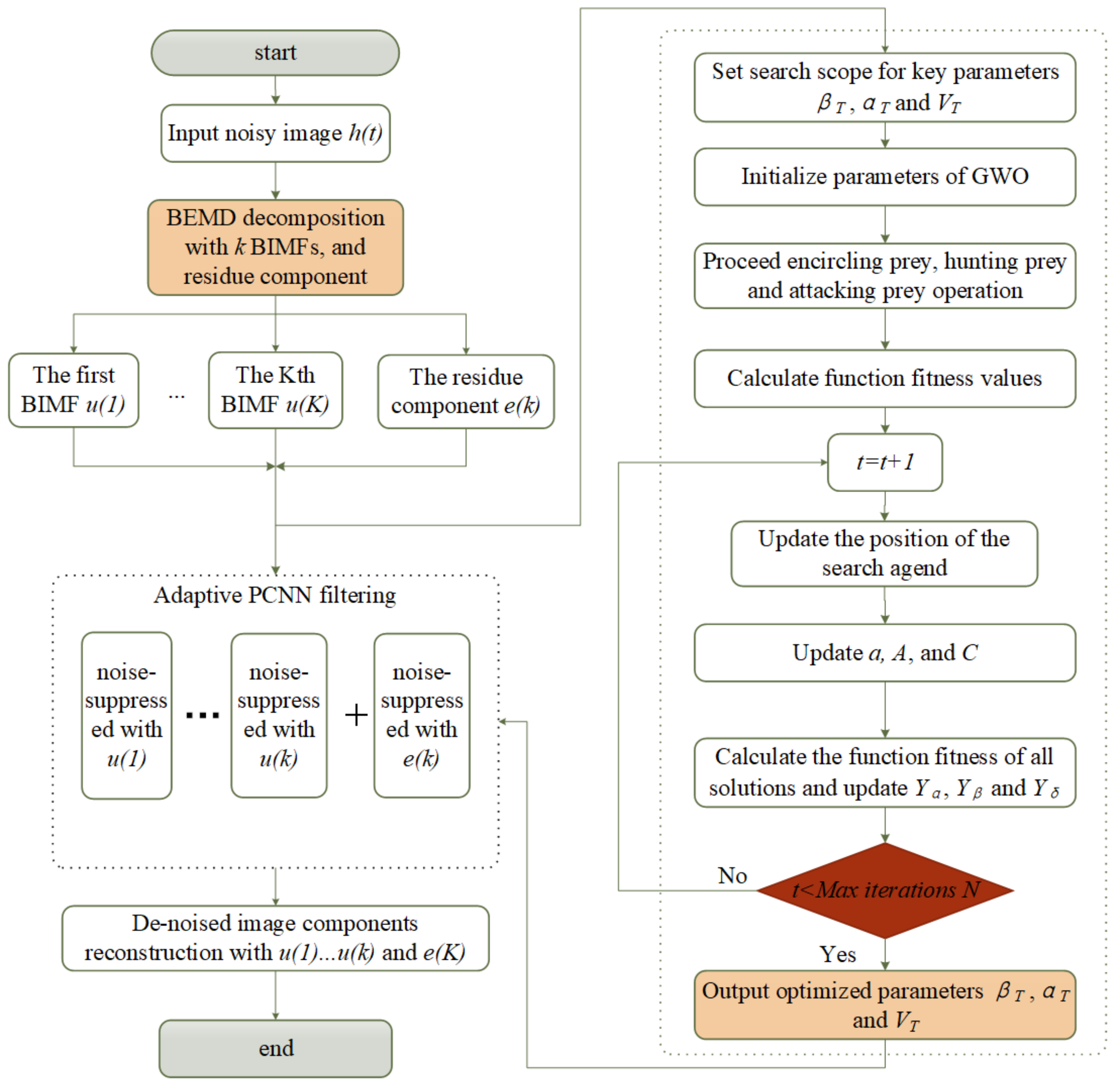
In this work, to provide further improvement in the accuracy of the search, the PCNN parameters are taken from pre-set ranges [17], where ${\alpha }_T$ and ${\beta }_T$ are both in the range between [0, 1.00], and VT is set over the range from 0 to 300.000. The maximum number of iterations $N=30$, the search agent number search Agent = 20, and the number of variables dim = 3 in the GWO algorithm. Using optimized parameters, the PCNN is used to perform component purification. Finally, the signal obtained contains the valid components of the original image. A detailed flowchart (shown in Figure 3) of the proposed noise elimination method is provided. To test the convergence rate of the GWO algorithm, a test fitting function is provided, and the whole search space from the 3D surface plot (Figure 4a) that corresponds to the function is shown, where $x_1,x_2\in \left[-100,100\right]$, and the number of $step=2$. The iteration number is set at 500. The GWO convergence curve is presented in Figure 4b, where the vertical coordinates represent the best fitness values selected by calculation of the tested function in the population region search. To demonstrate the GWO convergence advantages, we also applied two current methods, which are the GACA [17] and PSO algorithms [16], for comparison. As shown in Figure 4b, the number of iterations is set as 500 times, in order to conveniently and more clearly compare the convergence results. The iterative curves tell us that the GWO algorithm can complete convergence quicker than the PSO algorithm and is capable of accomplishing global search optimization in the curve trend analysis. The GACA has an unsatisfactory convergence delay performance, requiring excessively high iteration numbers, while the calculated function fitness value distribution is irregular, which also affects the assessment. To evaluate the optimization algorithms more comprehensively,

Table 1. The calculated function fitness values through different iterations and required run time for optimization by the PSO, GACA, and GWO.

Iterations	PSO		GACA		GWO
	BFV	T	BFV	T	BFV	T
20	1146.1940	0.02028	955.8790	0.1327	1381.7552	0.01928
50	22.2860	0.03127	5.7107	0.2156	88.7404	0.02600
80	6.6016	0.06410	1.8234	0.3124	13.8223	0.04532
120	2.8934	0.07290	1.2502	0.4133	2.2733	0.03903
200	0.1724	0.07631	0.4912	0.6303	1.7210	0.05433
250	0.06687	0.1040	0.2456	1.3923	1.2444	0.1011
300	0.009223	0.1586	0.0003280	1.8772	0.5071	0.1251
400	0.003017	0.2583	0.002050	2.3940	1.3801	0.1436
500	1.5440 × 10−5	0.3397	0.02507	3.4915	0.5012	0.1881

shows the best fitness values (BFV) through a range of different iterations from 20 to 500, along with the run time (T). In terms of run time, the GWO has a higher speed. The GACA iteration speed is relatively slow because of the larger influence of the combination factor. From the fitness values obtained, the ordering rule for these methods generally follows GWO > PSO > GACA. A table containing Algorithm 3 for the proposed hybrid image denoising algorithm, when the adaptive PCNN is combined with the GWO and BEMD, is shown below.

Algorithm 3 The Adaptive PCNN Optimized by the GWO and BEMD Algorithm

BEMD decomposition: Input raw image df Generate decomposed BIMF $u_k$ and residue $r_k$. Boundary treatment: Generate edge-symmetric extension, make the original image (m, n) change into (m + 6, n + 6); Initialize the PCNN parameters: Initialize ${\alpha }_T$, ${\beta }_T$, $v_T$ and $W_{ijkl}$ the number of pass N, step length ${\Delta }_t$; GWO algorithm implement: Keep each pixel in an unignited condition; Obtained optimized ${\alpha }_T$, ${\beta }_T$ and ${\nu }_T$ Contaminated points detection and treatment in PCNN: Calculate every neuron $L_{ij}\left[n\right]$ values in $3\times 3$ neighboring region using Equation (7) adjust the threshold using Equation (10); calculate the neuron internal modulation signal $E_{ij}\left[n\right]$ using Equation (9); if a neuron (i, j) is ignited in $3\times 3$ neighbor region and more than 4 adjacent neurons are unignited, the (i, j) pixels brightness will decline an ${\Delta }_t$ end; if a neuron (i, j) is unignited in $3\times 3$ neighbor region and more than 4 adjacent neurons are ignited, the (i, j) pixels brightness will increase a ${\Delta }_t$ end; Otherwise the pixels brightness values of the (i, j) won’t change end; Compare the $u_{ij}\left[n\right]$ values and $E_{ij}\left[n\right]$ values, record the neuron output, ignited or unignited; $N=N-1$, if $N\ne 0$, return to contaminated points detection and treatment Filtering processing: For further noise reduction, apply median filter to the treated image end; Otherwise, end. Reconstruct each component $u_k$ and $r_k$, and obtain the final denoising image

3. Experimental Results and Analysis

The effectiveness of the proposed PCNN-BEMD when combined with the GWO method can be verified experimentally. The best parameters for the PCNN can be obtained from GWO, from which noise separation can be obtained and a pre-denoising process can be completed; then, a median filter will be applied for noise reduction. The BEMD is performed within the PCNN to improve its performance.

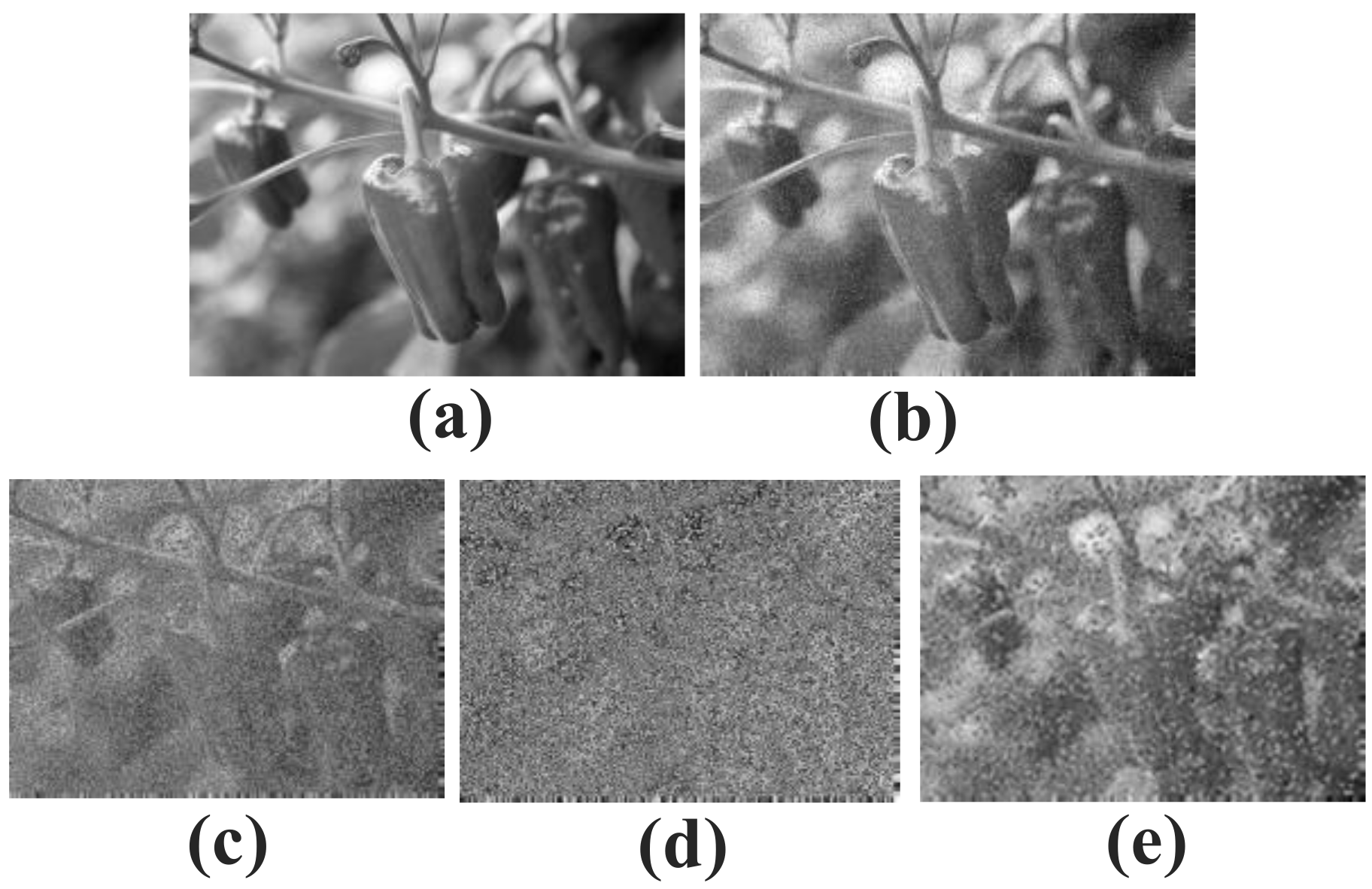
The experimental implementation results (Figure 5 and Figure 6) for the proposed method are validated. The original Lena image and the Pepper image are in JPG format and the original image sizes are $3\times 512\times 512$ and $3\times 750\times 1020$, respectively. The images were both conducted gray processing in advance then are preprocessed by decomposition using the BEMD. Consequently, the decomposed BIMFs and the corresponding residues can be presented. The original images have salt and pepper noise superimposed on them with density δ2 = 0.05, i.e., the percentage of the image area that contains the noise value. Based on observation of the polluted image, the original outlines and the details of these images cannot be distinguished clearly because of the noise interference. BIMFs 1 and 2 contain numerous noise points, such as the irregular black and white clouds of points. The residue contains a relatively small number of noise points, while also containing plentiful original details of both the image and the main frame. Therefore, each component should be purified using the PCNN filter.

Before PCNN filtering, the optimal parameters must be determined using the GWO. After the relevant calculation processes for the encircling, hunting and attacking operators, the values of ${\alpha }_T$, ${\beta }_T$, and $v_T$ that correspond to each component are presented (

Table 2. The experimentally obtained optimal parameters data for each decomposed component corresponding to the Lena and Pepper image.

Mode	Lena			Pepper
	αT1	βT1	VT1	αT2	βT2	VT2
BIMF1	0.107	0.260	273.858	0.0318	0.0344	229.263
BIMF2	0.0594	0.423	119.719	0.338	0.730	256.035
Residue	0.125	0.784	222.941	0.229	0.497	100.000

). Obviously, the parameters are different for each image component. However, there are no significant data rules between these parameters.

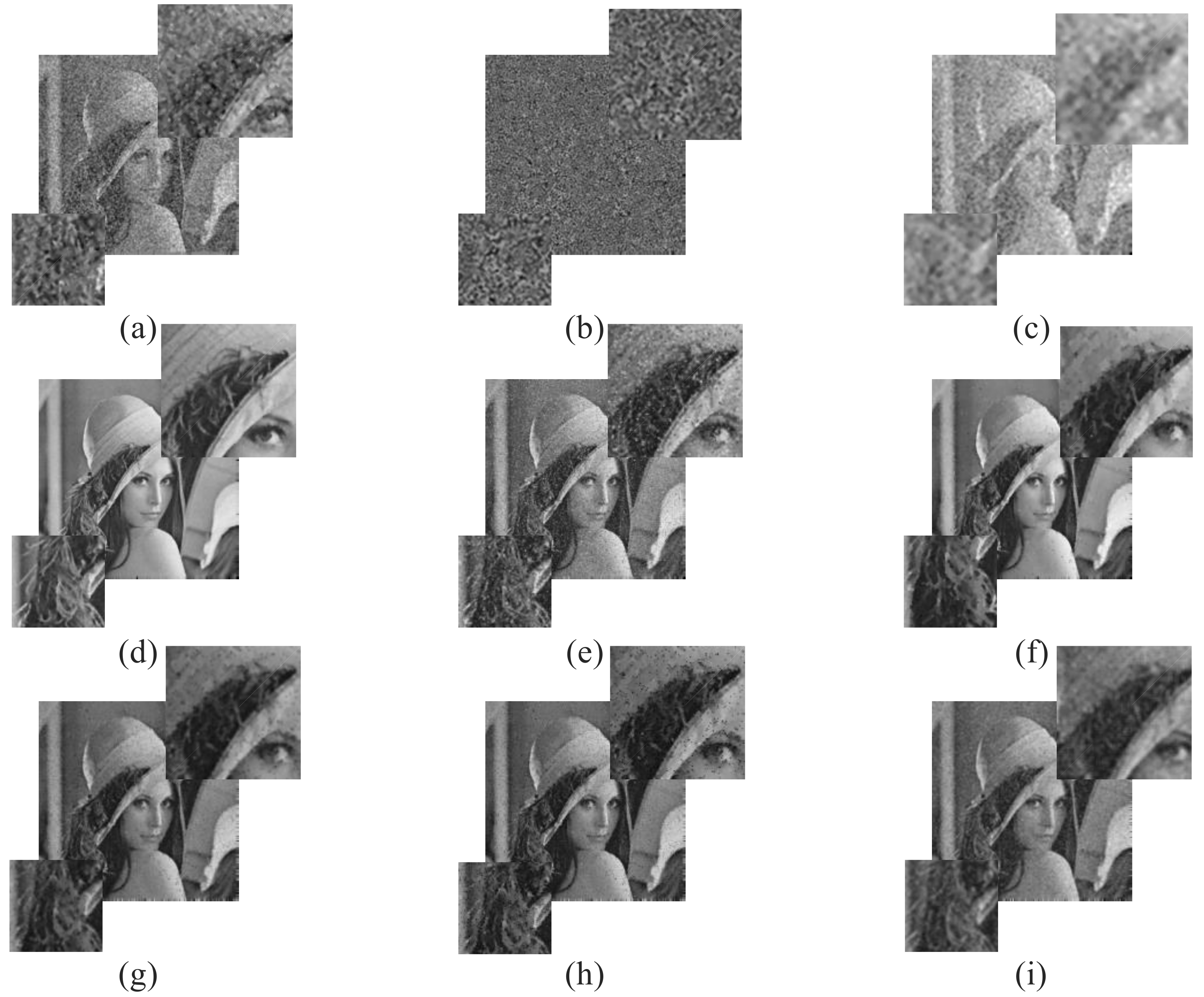
Using the calculated parameters above, optimized PCNN filtering is applied to the noise-polluted Lena and Pepper images for denoising. The noise suppression results for BIMFs 1 to 2 and the residue (Figure 7d–i and Figure 8d–i) show that the heavy salt and pepper noise is eliminated. The valid image details are extracted effectively, and the image outlines and edges are recovered well. Finally, the reconstructed images (Figure 7d and Figure 8d) with the decomposed components enable detailed comparison of the noise suppression effects of the different denoising methods, including the median filter, the particle swarm optimization method (PSO-PCNN), the conventional random PCNN (COR-PCNN) method, the genetic ant colony algorithm (GACA-PCNN) and the non-linear complex diffusion process technique (NLCDP) in the tBEMD domains (tBEMD-NLCDP). Observations indicate that our proposed BEMD-GWO-PCNN approach more than matches the other methods. When compared with the original images, the experimentally reconstructed images show a good performance in terms of the recovery of image details. However, the other methods appear to have processing blur or certain amounts of residual noise.

A quantitative analysis of the different de-noising methods is presented in

Table 3. Results from an experimental evaluation comparing indicator values of standard deviation (STD), mutual information (MI), structural similarity index measurement (SSIM) and peak signal to noise ratio (PSNR) of the unprocessed images with those from different noise reduction methods.

Results	Lena				Pepper
	STD	MI	SSIM	PSNR	STD	MI	SSIM	PSNR
Unprocessed image	28.042	0.679	0.109	13.853	5.684	1.436	0.106	10.241
BIMF 1	0.187	0.643	−0.107	6.581	5.671	0.100	−0.015	5.671
BIMF 2	14.619	0.078	0.034	6.840	7.241	0.413	0.023	5.685
Residue	36.361	1.305	0.186	15.749	11.029	1.644	0.286	15.357
BEMD-GWO-PCNN	53.316	2.368	0.788	23.159	17.774	4.262	0.607	21.774
GACA-PCNN	50.006	1.804	0.599	19.532	15.685	3.240	0.596	18.029
COR-PCNN	45.612	1.689	0.414	16.925	12.684	2.165	0.387	17.963
PSO-PCNN	48.469	1.971	0.683	20.007	15.357	2.514	0.439	20.684
Median filter	45.348	1.718	0.442	19.078	10.685	2.023	0.326	17.033
tBEMD-NLCDP	47.366	1.793	0.527	20.223	15.388	2.854	0.546	18.003

. The table clearly shows that the proposed BEMD-GWO-PCNN algorithm yields a better denoising performance, with higher STD and PSNR values, which means higher contrast with regard to each image’s pixel gray level and reduced noise content. In addition, the MI and SSIM values of the proposed method are higher than those of the other methods. Analysis of the indicators shows that the denoised image obtained using the proposed BEMD-GWO-PCNN algorithm has a higher degree of fitness with respect to the original image. The PSO-PCNN algorithm also provides an excellent denoising performance, which benefits greatly from the intelligent swarm model optimization used to improve the PCNN denoising performance. The GACA-PCNN algorithm can also produce a relatively good effect; nevertheless, the whole optimization algorithm is difficult to run because of multiple overlapping iterative combinations. Meanwhile, the above methods cannot achieve the desired goal in the image detail extraction. And the operation of the entire GACA-PCNN program is multi-regional and complex. The tBEMD-NLCDP method can also yield some results, the detail is well presented, but it did not perform well for salt and pepper noise removal. At the same time, the tBEMD-NLCDP method obviously lacks enough ability in the face of high-intensity noise.

To produce a more comprehensive analysis, different intensities of δ2 = 0.1, 0.2, and 0.3 for salt-pepper noise are added to the original Lena and Pepper images. In

Table 4. Comparison of the adaptive PCNN combined with BEMD method with other current denoising methods corresponding to different noise intensity values δ in Lena.

Lena		Noise Image	PSO-PCNN	GACA-PCNN	tBEMD-NLCDP	BEMD-GWO-PCNN
δ2 = 0.1	STD1	38.874	46.596	43.899	42.191	46.626
	MI1	1.612	2.877	1.983	2.487	3.147
	SSIM1	0.170	0.817	0.957	0.612	0.955
	PSNR1	15.343	28.153	33.426	27.143	34.691
δ2 = 0.2	STD2	35.421	38.945	46.937	36.487	54.672
	MI2	1.588	2.799	1.819	3.218	4.097
	SSIM2	0.0905	0.577	0.682	0.0667	0.806
	PSNR2	12.329	16.807	22.292	15.398	29.642
δ2 = 0.3	STD3	32.709	42.861	45.364	41.315	48.498
	MI3	1.097	2.614	1.864	2.446	2.695
	SSIM3	0.0605	0.726	0.592	0.782	0.793
	PSNR3	10.576	20.265	23.680	18.346	26.359

and

Table 5. Comparison of the adaptive PCNN combined with BEMD method with other current denoising methods corresponding to different noise intensity values δ in Pepper.

Pepper		Noise Image	PSO-PCNN	GACA-PCNN	tBEMD-NLCDP	BEMD-GWO-PCNN
δ2 = 0.1	STD1	45.605	51.573	48.157	49.253	51.685
	MI1	1.703	2.403	1.961	2.381	2.515
	SSIM1	0.0427	0.854	0.701	0.861	0.906
	PSNR1	15.246	32.224	26.358	30.269	32.362
δ2 = 0.2	STD2	42.539	50.633	45.078	44.328	51.954
	MI2	1.634	2.090	2.177	1.933	2.386
	SSIM2	0.0272	0.855	0.502	0.724	0.878
	PSNR2	12.274	24.009	28.086	27.913	29.966
δ2 = 0.3	STD3	40.205	50.552	52.705	49.251	53.256
	MI3	1.607	2.426	1.945	1.837	2.432
	SSIM3	0.0903	0.562	0.596	0.514	0.709
	PSNR3	10.566	23.823	20.817	22.037	24.108

, PSO-PCNN and GACA-PCNN are compared with our proposed BEMD-GWO-PCNN method to verify their noise reduction capabilities for high-intensity noise. From the data analysis, the proposed BEMD-GWO-PCNN method does provide a fairly good denoising effect. When compared with the original noisy images, the indicator values of the STD, MI, SSIM, and PSNR provide a good reflection of the image quality improvements produced by the noise reduction. The PSNR and STD values of the proposed algorithm are relatively high, which means lower noise residue. At the same time, the MI and SSIM values describe the degree of recovery of the image details. From the indicator data analysis, the BEMD-GWO-PCNN method enables effective image detail extraction and noise reduction. In the Lena and Pepper images, the PSO-PCNN, GACA-PCNN, tBEMD-NLCDP method and BEMD-GWO-PCNN methods all performed well. However, multiple experiments demonstrated that our method is more feasible and provides superior performance to the GACA-PCNN PSO-PCNN, and tBEMD-NLCDP methods. In fact, our method has shown that the noise interference is well eliminated, and that the extraction of the image stripe details is well completed. At the same time, the PSO-PCNN, GACA-PCNN and tBEMD-NLCDP method lacks enough ability in the face of high-intensity noise, whose performances are relatively weak.

4. Conclusions

With the aim of image noise suppression, an adaptive PCNN method optimized using the GWO and BEMD has been presented in this paper. Practical application of the proposed hybrid denoising algorithm has been achieved and yielded a better effect than other existing image denoising methods. In the proposed de-noising method, the PCNN filter is used for image denoising, while the GWO and BEMD are used as auxiliary algorithms to improve PCNN’s noise reduction effects. To solve the critical problem of the parameter optimization issue, the GWO has been applied to global optimization through screening and iteration processes to derive optimized parameters. As a conclusion, the proposed method can be targeted more effectively to eliminate each decomposed component when BEMD is used, and the decomposed components have been treated differently by the PCNN filtering with specific critical parameters.

Analyses of the denoising performance in the face of high-intensity noise has indicated that the faster parameter optimization convergence speed and better effects make it superior to other parameter optimization algorithms. The experimental outcomes analysis in the Pepper and Lena images have provided evidence for the effectiveness of the proposed BEMD-GWO-PCNN algorithm in image noise suppression applications. A higher PSNR value has represented the more valid statics preservation, which corresponds to more noise removal. Furthermore, our adopted indicators STD, MI, and SSIM are, in a high-level meaning, a closer degree to the size and distribution of the original image pixel points.

However, as the accuracy and effectiveness of our algorithms increase significantly, the running complexity will increase slightly. In the future, we hope that we can further improve the convergence speed and accuracy level of the algorithm in order to keep refined. In this paper, we only address salt and pepper noise suppression. Thus, it is necessary to promote the suppression of other noise. Additionally, how to realize real-time image noise reduction and reduce the operation running time as much as possible, are also topics to be studied carefully.