A Fast and Reliable Luma Control Scheme for High-Quality HDR/WCG Video

Featured Application

The proposed scheme is highly useful for high quality HDR imaging applications including cameras and post-production systems using HDR-10 media profile.

Abstract

The evolution of display technologies makes high dynamic range/wide color gamut (HDR/WCG) media of great interest in various applications including cinema, TV, blue-ray titles, and others. However, the HDR/WCG media format for consumer electronics requires the sampling rate conversion of chroma signals, resulting in a quality problem on the luminance perception of media, even without compression. In order to reduce such luminance perception problems, this paper proposes a fast and reliable luma control scheme which takes advantage of the bounds on the best luma value derived from the solution based on truncated Taylor series. Simulations performed for an extensive comparison study demonstrate that the proposed algorithm significantly outperforms the previous representative fast luma control schemes, resulting in almost the same quality of the iterative optimal solution with a fixed amount of computations per processing unit.

1. Introduction

High dynamic range and wide color gamut (HDR/WCG) video has recently received much attention due to its significant impact on the improvement of video quality by using a much higher contrast range, wider color primaries, and higher bit depth than conventional standard dynamic range (SDR) video. In order to facilitate the usage of such HDR/WCG video, standardization efforts have been made, including the production format of HDR-TV [1], the HDR electro-optical transfer function (EOTF) [2], the common media format for consumer electronics [3], and so on.

In dealing with such HDR/WCG video, chroma subsampling, which is a key component for a video preprocessing system, introduces a severe quality problem on subjective luminance perception. Several Moving Picture Experts Group (MPEG) contributions identified this problem [4,5], which is likely caused by the combination of the Y’CbCr 4:2:0 nonconstant luminance (NCL) format with the highly nonlinear transfer function of [2]. Appearing as a type of false contouring or noise-like speckles in the smooth area, the artifacts of this problem sometimes become very annoying to viewers even without compression.

To ameliorate such artifacts from chroma subsampling, various luma control schemes have been suggested in the literature [6,7,8,9,10]. Luma control implies an intentional change of luma signal, which is not subsampled, for the purpose of reducing the perception error introduced by chroma subsampling. In one category of such luma control schemes, the perception error is defined in a nonlinear light domain using the signals obtained after the application of an optoelectrical transfer function (OETF) and quantization [6,7]. The schemes in this category can be easily applied to conventional imaging systems, but the incorporated perception error could not be correctly matched to the human visual system (HVS) because most HVS measures (i.e., CIEDE2000 [11]) are defined in the linear light domain.

For this reason, the other category of luma control methods optimizes the error function defined in the linear light domain. One solution proposed in [8] was to simulate the NCL Y’CbCr 4:2:0 signal conversion followed by chroma upsampling for iterating over different luma values to choose the best one, resulting in the closest linear luminance to that of the original 4:4:4 signal. By searching for the best possible luma value, the solution achieved a significant linear luminance gain (i.e., more than 17 dB of tPSNR-Y in [8]) over the plain NCL Y’CbCr 4:2:0 signal. However, the iterative nature of searching, even done quickly with the tight bounds (also proposed in [8]), requires an uneven amount of complex computations per processing unit. To avoid such iterations for luma control, Norkin proposed a closed form solution in [9] based on a truncated Taylor series approximation for the nonlinear HDR EOTF function. This solution requires a fixed number of operations per pixel and thus is well suited for a real-time and/or hardware implementation of the NCL Y’CbCr 4:2:0 HDR system, but its performance is limited for some videos that have highly saturated colors. To fill the performance gap between the above two schemes, the authors proposed an enhanced fast luma control algorithm in [10]. Based on the fact that the linear approximation for a convex function using truncated Taylor series is always less than the function value, the enhanced luma control scheme modifies the linear approximation, resulting in a meaningful gain over the previous fast scheme. However, there still remains a nonnegligible performance gap and the algorithm requires a parameter which is not determined automatically.

Considering the pros and cons of these previous luma control schemes, this paper focuses on an interesting question: can we design a linear approximation of the nonlinear HDR EOTF which can provide a similar performance to that of the iterative luma control method while being free of the limiting factors in real-time or hardware implementation such as the adaptive selection of control parameters or the uneven amount of required computations? To answer this question, we first analyzed the errors involved in the closed form solution of [9], which derives an upper and a lower bound on the optimal luma value from the convexity property of the EOTF function. Then, we tried various linear approximations employing the derived bounds to design an efficient linear approximation of the nonlinear EOTF function. Based on the trials, we argue that the straight lines passing two points on the EOTF curve are quite useful, where one is the position of the original 4:4:4 signal and the other is the point somewhere between the derived lower and upper bounds. Via the modification of the closed form solution using these straight lines, we show that the proposed scheme can provide nearly the same quality of the iterative solution without any limiting factors in its real-time or hardware implementation.

The rest of this paper is organized as follows. Section 2 describes the problem of luma control and the approaches taken by the previous representative algorithms. Then, in Section 3, we investigate the luminance perception error minimized by the fast solution in [9], resulting in two new bounds on the position of the best luma value. This section also explains the proposed linear approximation using the derived two bounds. Simulations for an extensive comparison study and their results are presented in Section 4, and then we conclude this paper in Section 5.

2. Luma Control Problem

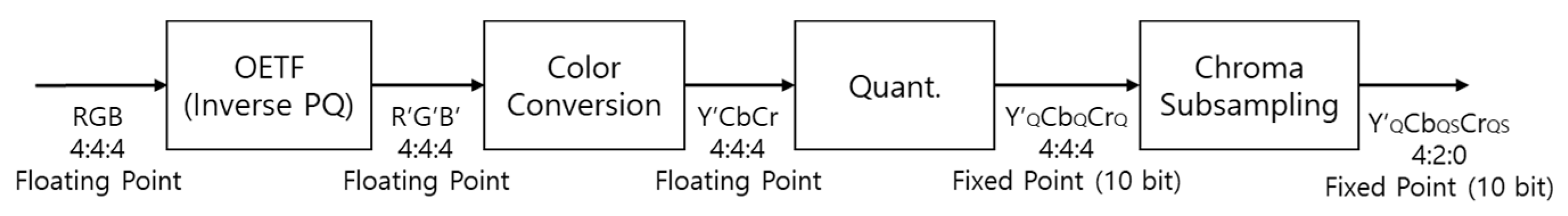
To define the luma control problem, let $R,G,B$ denote the original pixel values in the linear light domain, which are to be transformed to NCL Y’CbCr 4:2:0 pixel values. For HDR-10 video [3], this transformation employs the inverse ST.2084 [2] Perceptual Quantizer (PQ), the Y’CbCr color-space conversion, the narrow-band 10-bit quantization, and chroma subsampling in this order, as described in [12] and depicted in Figure 1.

After the processing steps, such as video encoding, transmission, reception, and decoding, the reconstructed NCL Y’CbCr 4:2:0 video is supposed to be transformed back to the RGB display signal in the linear light domain. The postprocessing for this transformation shall comprise the stages, which are exactly the inverses of the corresponding preprocessing blocks. Hence, this processing involves chroma upsampling, inverse 10-bit quantization, RGB color-space conversion, and then ST.2084 EOTF. For now, in order to consider the artifacts caused by chroma subsampling, let us leave the processing blocks from video encoding to decoding behind. If we denote by $\widehat{R},\widehat{G},\widehat{B}$ the reconstructed output pixel values of the postprocessing, we can define the luminance error by

$$E={\left\{w_R\left(\widehat{R}-R\right)+w_G\left(\widehat{G}-G\right)+w_B\left(\widehat{B}-B\right)\right\}}^2,$$

(1)

where $\left(w_R,w_G,w_B\right)$ represents the contribution of each linear light component to luminance and is given by (0.2126, 0.7152, 0.0722) for BT.709 [13] and (0.2627, 0.6780, 0.0593) for BT.2020 [14] color gamut. Translation of this error to the one with nonlinear reconstructed signals provides

$$E={\left\{w_R\left(L\left({\widehat{R}}^{\prime }\right)-L\left(R^{\prime }\right)\right)+w_G\left(L\left({\widehat{G}}^{\prime }\right)-L\left(G^{\prime }\right)\right)+w_B\left(L\left({\widehat{B}}^{\prime }\right)-L(B^{\prime })\right)\right\}}^2,$$

(2)

where the “prime” notation, as a well-known convention, illustrates that the signal is in the “nonlinear” domain, and $L(·)$ denotes the ST 2084 EOTF, which is defined by

$$L\left(X\right)={\left[\frac{\max \left(\left(X^{1/m}-c_1\right),0\right)}{c_2-c_3·X^{1/m}}\right]}^{1/n},$$

(3)

where $m=78.84375$, $n=0.1593017578$, $c_1=0.8359375$, $c_2=18.8515625$, and $c_3=18.6875$.

For further investigation of the reconstructed nonlinear signal, $\left({\widehat{R}}^{\prime },{\widehat{G}}^{\prime },{\widehat{B}}^{\prime }\right)$, let us denote the chroma subsampling errors by $\Delta C_b$ and $\Delta C_r$, such that

$${\widehat{C}}_b=C_b+\Delta C_b,{\widehat{C}}_r=C_r+\Delta C_r,$$

(4)

where $\left({\widehat{C}}_b,{\widehat{C}}_r\right)$ and $\left(C_b,C_r\right)$ represent the reconstructed and the original chroma signal pairs in nonlinear 4:4:4 format, respectively. In order to compensate for these subsampling errors, if we assume that the original luma value, $Y^{\prime }$, is adjusted to a new one, ${\widehat{Y}}^{\prime }=Y^{\prime }+\Delta Y^{\prime }$, then the reconstructed signal, $\left({\widehat{R}}^{\prime },{\widehat{G}}^{\prime },{\widehat{B}}^{\prime }\right)$, or equivalently, the reconstruction difference, $\left(\Delta R,\Delta G,\Delta B\right)=\left({\widehat{R}}^{\prime },{\widehat{G}}^{\prime },{\widehat{B}}^{\prime }\right)-\left(R^{\prime },G^{\prime },B^{\prime }\right)$, can be represented by

$$\left[\begin{array}{c}{\widehat{R}}^{\prime }\\ {\widehat{G}}^{\prime }\\ {\widehat{B}}^{\prime }\end{array}\right]=\left[\begin{array}{ccc}1& 0& a_{RCr}\\ 1& a_{GCb}& a_{GCr}\\ 1& a_{BCb}& 0\end{array}\right]\left[\begin{array}{c}{\widehat{Y}}^{\prime }\\ {\widehat{C}}_b\\ {\widehat{C}}_r\end{array}\right]or\left[\begin{array}{c}\Delta R\\ \Delta G\\ \Delta B\end{array}\right]=\left[\begin{array}{ccc}1& 0& a_{RCr}\\ 1& a_{GCb}& a_{GCr}\\ 1& a_{BCb}& 0\end{array}\right]\left[\begin{array}{c}\Delta Y^{\prime }\\ \Delta C_b\\ \Delta C_r\end{array}\right],$$

(5)

where $\left(a_{RCr},a_{GCb},a_{GCr},a_{BCb}\right)$ means the contribution of a chroma component for each color and is given by (1.5748, −0.1873, −0.4681, 1.8556) for BT.709 and (1.4746, −0.1646, −0.5714, 1.8814) for BT.2020. This shows the adjusted luma value, ${\widehat{Y}}^{\prime }$, controls the nonlinear domain reconstruction, $\left({\widehat{R}}^{\prime },{\widehat{G}}^{\prime },{\widehat{B}}^{\prime }\right)$, and thus determines the luminance error given in (2). Hence, the luma control problem is to find the best luma value that produces the minimum luminance error of (2).

The iterative luma control scheme in [8] searches for the best compensation using the bisection method with their proposed bounds on the optimal luma value. The iterative nature of the scheme comes from the nonlinearity of $L\left({\widehat{X}}^{\prime }\right),{\widehat{X}}^{\prime }\in \left\{{\widehat{R}}^{\prime },{\widehat{G}}^{\prime },{\widehat{B}}^{\prime }\right\}$ in (2), resulting in its repeated and complex computations for each candidate luma value. To get rid of the iterative nature of the luma control scheme, [9] proposed an approximation of $L\left({\widehat{X}}^{\prime }\right)$ based on a truncated Taylor series, such that

$$L\left({\widehat{X}}^{\prime }\right)=L\left(X^{\prime }+\Delta X\right)=L\left(X^{\prime }\right)+L^{\prime }\left(X^{\prime }\right)·\Delta X,X^{\prime }\in \left\{R^{\prime },G^{\prime },B^{\prime }\right\},$$

(6)

where $R^{\prime },G^{\prime },B^{\prime },$ are the original pixel values in nonlinear RGB color space and $L^{\prime }(·)$ denotes the derivative of the EOTF, $L(·)$. This approximation, after combined with (5) and (2), provides an optimal luma value, ${\widehat{Y}}_F^{\prime }$, as a closed form solution of

$${\widehat{Y}}_F^{\prime }=\frac{w_R·L^{\prime }\left(R^{\prime }\right)·e_R+w_G·L^{\prime }\left(G^{\prime }\right)·e_G+w_B·L^{\prime }\left(B^{\prime }\right)·e_B}{w_R·L^{\prime }\left(R^{\prime }\right)+w_G·L^{\prime }\left(G^{\prime }\right)+w_B·L^{\prime }\left(B^{\prime }\right)},$$

(7)

where

$$\begin{array}{c}{e}_R=Y^{\prime }-a_{RCr}\Delta C_r\\ e_G=Y^{\prime }-a_{GCb}\Delta C_b-a_{GCr}\Delta C_r\\ e_B=Y^{\prime }-a_{BCb}\Delta C_b\end{array}$$

(8)

This fast scheme is very simple and no longer iterative but shows limited performance for some videos having highly saturated colors. As a reason for this performance limitation, [10] pointed out that the approximation of (6) can be severely limited when $L\left(X^{\prime }\right)$ has a high curvature at the point $X^{\prime }$ and when $\Delta X$ is not small. To fill the performance gap between the above two luma control schemes, a modified linear approximation was proposed in [10], such that

$$L\left({\widehat{X}}^{\prime }\right)=L\left(X^{\prime }+\Delta X\right)=\left[L\left(X^{\prime }\right)+f_X\left(X^{\prime },\Delta X_F\right)\right]+s\left(X^{\prime },\Delta X_F\right)·\Delta X,X^{\prime }\in \left\{R^{\prime },G^{\prime },B^{\prime }\right\},$$

(9)

where $\Delta X_F$ is the resulting value from (5) with (7), specifically,

$$\left[\begin{array}{c}\Delta R_F\\ \Delta G_F\\ \Delta B_F\end{array}\right]=\left[\begin{array}{ccc}1& 0& a_{RCr}\\ 1& a_{GCb}& a_{GCr}\\ 1& a_{BCb}& 0\end{array}\right]\left[\begin{array}{c}{\widehat{Y}}_F^{\prime }-Y^{\prime }\\ {\widehat{C}}_b-C_b\\ {\widehat{C}}_r-C_r\end{array}\right]$$

(10)

The parameters $s\left(X^{\prime },\Delta X_F\right)$ and $f_X\left(X^{\prime },\Delta X_F\right)$ in (9) are defined by

$$s\left(X^{\prime },\Delta X_F\right)=\left[L\left(X^{\prime }+\left|\Delta X_F\right|\right)-L\left(X^{\prime }-\left|\Delta X_F\right|\right)\right]/2\left|\Delta X_F\right|,$$

(11)

$$f_X\left(X^{\prime },\Delta X_F\right)=r·\left[L\left(X^{\prime }-\left|\Delta X_F\right|\right)+L\left(X^{\prime }+\left|\Delta X_F\right|\right)-2L\left(X^{\prime }\right)\right]/2,$$

(12)

where $r$ is a nonautomatic parameter, called the “reduction factor”, in the range of (0,1).

3. Linear Approximation of EOTF

In the linear model of EOTF, like the truncated Taylor series in (6), the accuracy of the model can be significantly enhanced by knowledge of the location of the target(s) to be approximated. The modification of (9) is one example of such an enhancement. In this section, for more precise approximation of the ST.2084 EOTF, we investigate the errors of the fast solution (7), resulting in two, upper and lower, bounds on the location of the optimal luma value.

3.1. Limitations of Fast Luma Control

By inserting (6) into (2) and then combining (5) with (8) for $\Delta X,X\in \left\{R,G,B\right\},$ the luminance perception error can be represented by

$$\begin{array}{ll}E& ={\left[{\displaystyle {\displaystyle \sum }_{X\in \left\{R,G,B\right\}}}{w}_X\left(L\left(X^{\prime }+\Delta X\right)-L\left(X^{\prime }\right)\right)\right]}^2\\ & ={\left[{\displaystyle {\displaystyle \sum }_{X\in \left\{R,G,B\right\}}}{w}_X\left(L^{\prime }\left(X^{\prime }\right)\Delta X\right)\right]}^2\\ & ={\left[{\displaystyle {\displaystyle \sum }_{X\in \left\{R,G,B\right\}}}{w}_X\left(L^{\prime }\left(X^{\prime }\right)\left(\widehat{Y^{\prime }}-e_X\right)\right)\right]}^2\end{array}$$

(13)

The luma value, ${\widehat{Y}}_F^{\prime }$, in (7) is the solution minimizing (13) and we can easily identify that this minimum error value equals zero, which was attained by the approximation of the EOTF values $L\left(X^{\prime }+\Delta X_F\right)$ using (6), with $\Delta X_F\in \left\{\Delta R_F,\Delta G_F,\Delta B_F\right\}$ given in (10). Now, let us denote this approximated quantity by ${\widehat{X}}_F$ and its corresponding nonlinear quantity by ${{\widehat{X}}^{\prime }}_F$, specifically,

$${\widehat{X}}_F=L\left(X^{\prime }\right)+L^{\prime }\left(X^{\prime }\right)·\Delta X_F\mathrm{and}{{\widehat{X}}^{\prime }}_F=L^{-1}\left({\widehat{X}}_F\right),$$

(14)

where $L^{-1}(·)$ is the inverse of the EOTF given in (3) and the position of each quantity is depicted in Figure 2. Since the zero minimum, achieved by the $\Delta X_F$, is the lowest possible error of the luminance perception in (2), if we can find a luma value ${\widehat{Y}}^{\prime }$ producing the quantity ${{\widehat{X}}^{\prime }}_F$ (i.e., via (5)) for all the color components at the same time, then this value shall be the optimal one and be the same as that of the iterative solution. However, $\Delta X$ defined in (5) and ${\widehat{Y}}^{\prime }$ are with equal spacing (which means that if ${\widehat{Y}}^{\prime }$ is changed by an amount, then $\Delta X_F$ for all the color components are also changed by the same amount at the same time), but the distances from $X^{\prime }$ to ${{\widehat{X}}^{\prime }}_F$ for each color component are not guaranteed to be the same, hence, the existence of such ${\widehat{Y}}^{\prime }$ is not generally possible.

Instead, let us now consider the luma value ${{\widehat{Y}}^{\prime }}_{X\left(F\right)}$ producing the quantity ${{\widehat{X}}^{\prime }}_F$ for each color component, and the minimum and maximum values among ${\left\{{{\widehat{Y}}^{\prime }}_{X\left(F\right)}\right\}}_{X=R,G,B}$. From $\Delta X={\widehat{Y}}^{\prime }-e_X,X\in \left\{R,G,B\right\}$, we can get such ${{\widehat{Y}}^{\prime }}_{X\left(F\right)}$ as

$${{\widehat{X}}^{\prime }}_F-X^{\prime }={{\widehat{Y}}^{\prime }}_{X\left(F\right)}-e_X\mathrm{or}{{\widehat{Y}}^{\prime }}_{X\left(F\right)}={{\widehat{X}}^{\prime }}_F-X^{\prime }+e_X,X\in \left\{R,G,B\right\},$$

(15)

and

$${{\widehat{Y}}^{\prime }}_{min}=\min \left\{{{\widehat{Y}}^{\prime }}_{X\left(F\right)}\right\},{{\widehat{Y}}^{\prime }}_{max}=\max \left\{{{\widehat{Y}}^{\prime }}_{X\left(F\right)}\right\},X\in \left\{R,G,B\right\}$$

(16)

Then, if we further consider a luma value, ${{\widehat{Y}}^{\prime }}_a$, which is larger than the above ${{\widehat{Y}}^{\prime }}_{max}$ (i.e., ${{\widehat{Y}}^{\prime }}_a\ge {{\widehat{Y}}^{\prime }}_{max}$), the reconstructed RGB signal, ${{\widehat{X}}^{\prime }}_a$, via (5) can be represented by

$${{\widehat{X}}^{\prime }}_a={{\widehat{X}}^{\prime }}_{max}+{\delta }_{X\left(a\right)}={{\widehat{X}}^{\prime }}_F+{\delta }_{X\left(max\right)}+{\delta }_{X\left(a\right)},X\in \left\{R,G,B\right\},$$

(17)

where ${{\widehat{X}}^{\prime }}_{max}$ denotes the reconstructed RGB values from the corresponding ${{\widehat{Y}}^{\prime }}_{max}$, and ${\delta }_{X\left(max\right)},{\delta }_{X\left(a\right)}\ge 0$ for all $X$, because $\Delta X={\widehat{Y}}^{\prime }-e_X,X\in \left\{R,G,B\right\}$ and ${{\widehat{Y}}^{\prime }}_a\ge {{\widehat{Y}}^{\prime }}_{max}$. Hence, the luminance error introduced by this luma value can be represented by

$$\begin{array}{ll}E\left({{\widehat{Y}}^{\prime }}_a\right)& ={\left[{\displaystyle {\displaystyle \sum }_{X\in \left\{R,G,B\right\}}}{w}_X\left(L({\widehat{X}}^{\prime }{}_F)-L(X^{\prime })\right)+w_X\left(L({\widehat{X}}^{\prime }{}_F+{\delta }_{X\left(max\right)}+{\delta }_{X\left(a\right)})-L({\widehat{X}}^{\prime }{}_F)\right)\right]}^2\\ & ={\left[{\displaystyle {\displaystyle \sum }_{X\in \left\{R,G,B\right\}}}{w}_X\left(L({\widehat{X}}^{\prime }{}_F+{\delta }_{X\left(max\right)}+{\delta }_{X\left(a\right)})-L({\widehat{X}}^{\prime }{}_F)\right)\right]}^2,\end{array}$$

(18)

and the convexity of $L(·)$ illustrates $0\le E\left({{\widehat{Y}}^{\prime }}_{max}\right)\le E\left({{\widehat{Y}}^{\prime }}_a\right)$, which shows that ${{\widehat{Y}}^{\prime }}_{max}$ is an upper bound on the optimal luma value.

Using the same procedures with ${{\widehat{Y}}^{\prime }}_{min}$ and ${{\widehat{Y}}^{\prime }}_b$ (${{\widehat{Y}}^{\prime }}_b\le {{\widehat{Y}}^{\prime }}_{min}$), we can get the luminance perception error for the luma value, ${{\widehat{Y}}^{\prime }}_b$, such that

$$E\left({{\widehat{Y}}^{\prime }}_b\right)={\left[{\displaystyle \sum }_{X\in \left\{R,G,B\right\}}{w}_X\left(L({\widehat{X}}^{\prime }{}_F-{\delta }_{X\left(min\right)}-{\delta }_{X\left(b\right)})-L({\widehat{X}}^{\prime }{}_F)\right)\right]}^2,$$

(19)

where the convexity of $L(·)$, again, establishes $0\le E\left({{\widehat{Y}}^{\prime }}_{min}\right)\le E\left({{\widehat{Y}}^{\prime }}_b\right)$, which means that ${{\widehat{Y}}^{\prime }}_{min}$ is a lower bound on the optimal luma value.

3.2. Proposed Linear Approximation

In order to exploit the derived bounds for the linear approximation of EOTF, let us first consider the straight line passing the nonlinear and linear pair of the original color signal, $\left(X^{\prime },X\right)$, and the pair of the reconstructed color signal from ${{\widehat{Y}}^{\prime }}_{min}$, $\left({{\widehat{X}}^{\prime }}_{min},{\widehat{X}}_{min}\right)$, where $X\in \left\{R,G,B\right\}$. If we denote the slope of this line by $s_X$, then the EOTF for each reconstructed signal, ${{\widehat{X}}^{\prime }}_{min}\le {\widehat{X}}^{\prime }\le {{\widehat{X}}^{\prime }}_{max}$, can be represented by

$$L\left({\widehat{X}}^{\prime }\right)=L\left(X^{\prime }\right)+s_X·\Delta X+{\delta }_{{\widehat{X}}^{\prime }}$$

(20)

where $\Delta X={\widehat{X}}^{\prime }-X^{\prime }$ and ${\delta }_{{\widehat{X}}^{\prime }}$ denote the error between the EOTF and the considering straight line at ${\widehat{X}}^{\prime }$. Note that this representation is not an approximation of the EOTF with the appropriate value of ${\delta }_{{\widehat{X}}^{\prime }}$ which is always positive for every ${\widehat{X}}^{\prime }$ satisfying ${{\widehat{X}}^{\prime }}_{min}\le {\widehat{X}}^{\prime }\le {{\widehat{X}}^{\prime }}_{max}$ because of the monotonically increasing nature of the EOTF. With this representation, the minimization of (2) yields the optimum solution of

$${\widehat{Y}}_O^{\prime }=\frac{{{\displaystyle \sum }}_{X\in \left\{R,G,B\right\}}{w}_X{s}_X{e}_X}{{{\displaystyle \sum }}_{X\in \left\{R,G,B\right\}}{w}_X{s}_X}-\Delta ,\Delta =\frac{{{\displaystyle \sum }}_{X\in \left\{R,G,B\right\}}{w}_X{\delta }_{{\widehat{X}}^{\prime }}}{{{\displaystyle \sum }}_{X\in \left\{R,G,B\right\}}{w}_X{s}_X}$$

(21)

which comprises the linear approximation using the considering straight line in the first part and the following error correction term of $\Delta$. Hence, (21) shows the optimal solution ${\widehat{Y}}_O^{\prime }$ is always smaller than the solution from the straight line passing the two points $\left(X^{\prime },X\right)$ and $\left({{\widehat{X}}^{\prime }}_{min},{\widehat{X}}_{min}\right)$. Likewise, with the straight line passing the two points $\left(X^{\prime },X\right)$ and $\left({{\widehat{X}}^{\prime }}_{max},{\widehat{X}}_{max}\right)$ for each color $X\in \left\{R,G,B\right\}$, we can observe that true optimum is always larger than the approximate solution using the line.

Based on these two observations, we decided to use the straight line passing the two points $\left(X^{\prime },X\right)$ and $\left({{\widehat{X}}^{\prime }}_M,{\widehat{X}}_M\right)$ for each color $X\in \left\{R,G,B\right\}$ as the proposed linear approximation of the EOTF, where

$${\widehat{X}}_M=\left(a·{\widehat{X}}_{min}+b·{\widehat{X}}_{max}\right)/\left(a+b\right)\mathrm{and}{{\widehat{X}}^{\prime }}_M=L^{-1}\left({\widehat{X}}_M\right)$$

(22)

With this proposed linear approximation, the proposed luma value will be

$${\widehat{Y}}_P^{\prime }=\frac{{{\displaystyle \sum }}_{X\in \left\{R,G,B\right\}}{w}_X{s}_X{e}_X}{{{\displaystyle \sum }}_{X\in \left\{R,G,B\right\}}{w}_X{s}_X},s_X=\frac{{\widehat{X}}_M-X}{{{\widehat{X}}^{\prime }}_M-X^{\prime }}$$

(23)

4. Simulations and Results

To evaluate the performance of the proposed algorithm, an extensive comparison study was conducted using the previous luma control schemes explained in Section 2. The comparison is based on the pre-encoding and post-decoding processes defined in [12], with the downsampling filter, $f_0$, having the filter coefficients of (1/8, 6/8, 1/8). Tested video sequences are shown in Figure 3, where the first three (denoted by “Fireeater”, “Market”, and “Tibul”) are the BT.709 HDR video sequences used before in MPEG [15] and the last five sequences (denoted by “Beerfest”, “Carousel”, “Cars”, “Fireplace”, and “Showgirl”) are the BT.2020 HDR sequences chosen from [16]. In contrast to the MPEG sequences, some of the chosen BT.2020 sequences have multiple shots of a scene with too many frames (more than 2000) for simulation. Thus, we further selected a representative 200–400-frames-long portion of each sequence for the performed simulations. Detailed information on these selections and the characteristics of each test sequence are summarized in

Table 1. Characteristics of the tested HDR/WCG video sequences.

Name	Original File Name	Frames	Characteristics
Fireeater	FireEater2Clip4000r1_1920x1080p_25_hf_709_444_xxxxx.exr	00000–00199	low-key scene
Market	Market3Clip4000r2_1920x1080p_50_hf_709_444_xxxxx.exr	00000–00399	high color saturation
Tibul	Tibul2Clip4000r1_1920x1080_30_hf_709_444_xxxxx.exr	00000–00239	high-contrast scene
Beerfest	beerfest_lightshow_xxxxxx.tif	102352–102751	moving lights (color)
Carousel	carousel_fireworks_xxxxx.tif	95790–96089	moving lights (color)
Cars	cars_fullshot_xxxxxx.tif	132340–132539	sunlight scene
Fireplace	fireplace_xxxxx.tif	92775–92974	low-key scene
Showgirl	showgirl_01_xxxxxx.tif	235636–235935	high-contrast scene

NOTE: ‘xxxxx’ or ‘xxxxxx’ means the frame number of five or six digits.

.

All the test videos were of the same 1920 × 1080 resolution, maximum luminance of 4000 cd/m², and large amount of highly saturated colors. The color saturation was the most prominent property for the test sequences “Market”, “Beerfest”, and “Carousel”, which had highly saturated colors around all three color gamut boundaries, while the others had one or two. The sequences “Fireeater” and “Fireplace” were low-key scenes (filmed in low-key) with flames covering a wide range of color temperatures. The “Cars” sequence showed directional sunlight on a black car, resulting in glare on the car bonnet and windows, with dark shades under the car. Finally, the “Tibul” and “Showgirl” sequences contained object(s) exposed to the maximum luminance, resulting in extremely high-contrast images. The characteristics of the test sequences described here are also summarized in Table 1.

As an objective measure for the performance comparison of luma control schemes, we used the tPSNR, defined in the Annex F of [15], on the luminance signal (i.e., tPSNR-Y) and on the overall XYZ color signal (i.e., tPSNR-XYZ). The tPSNR measure is a new metric for HDR material involving the color conversion to CIE XYZ space and the average of two transfer functions, ST.2084 and Philips, for the calculation of PSNR.

Figure 4 summarizes the simulation results, where each number represents the tPSNR value averaged over all the frames of each test sequence. First, from each subfigure, we can easily identify that the performance difference is larger in tPSNR-Y (i.e., in Figure 4a) than in tPSNR-XYZ (i.e., in Figure 4b). This result is attributed to the objective function of luma control (i.e., Equation (1)), which concerns only the luminance perception error. Luma control optimizes such luminance error by modifying luma values and thereby directly enhances the luminance perception (i.e., tPSNR-Y) while indirectly enhancing the reconstructed color components (i.e., the $\widehat{R},\widehat{G},\widehat{B}$, in Equation (1)). Because of the weights, $\left(w_R,w_G,w_B\right)$ in the objective function, the improvement of tPSNR-X (closely related to the red color) is usually larger than that of tPSNR-Z (closely related to the blue color), and these indirect improvements are much less than that of tPSNR-Y. This limited improvement on tPSNR-X and tPSNR-Y restricts the difference of tPSNR-XYZ performance among tested luma control algorithms. One interesting point in the tPSNR-XYZ result given in Figure 4b is that the averaged result of the proposed scheme is better than that of the “Iterative” scheme (which is regarded as the optimal solution for luminance perception), although the gain is only 0.01 dB. This phenomenon tells us that better luminance perception may not always provide better overall signal perception, which justifies a new direction of luma control research based on a better perception metric or incorporating chroma modifications.

Now, let us examine the tPSNR-Y performance of the proposed algorithm. The “No Control” case in the figure is the conventional signal conversion using the NCL Y’CbCr4:2:0 format without luma control. If we compare the “Average” result of each luma control with that of this “No Control” case, we can identify that the proposed scheme achieved the tPSNR-Y improvement of 14.79 dB on average, while the “Fast” and the “E-Fast” schemes achieved 10.73 and 13.49 dB, respectively. On a sequence basis, the proposed luma control scheme enhanced the “Fast” and the “E-Fast” algorithms by up to 7.44 and 3.53 dB on the “Fireplace” and on “Market” sequences, respectively. One important observation here about these improvements is that there is no case of negative improvement. The proposed scheme is, on average, always superior to the compared previous fast luma control algorithms in all test sequences. Compared with the “Iterative” case (i.e., the optimal case), the tPSNR-Y of the proposed scheme is less than only 0.04 dB on average, indicating that the proposed scheme achieves nearly the same performance. However, we must note that nearly the same performance comes without iterations, i.e., there is no uneven amount of computations per pixel, which can be of great help to the hardware implementation of the proposed algorithm. Finally, let us look into the numbers inside the brackets in the “E-Fast” row of Figure 4a. They are the reduction factors, $r$, in (12), which were chosen as the best for each test sequence. As shown in the subfigure, the values are quite different for each test sequence (i.e., hard to use a fixed value) and the factor is known to have a great impact on the reconstruction quality (i.e., around 2 dB on average) [10]. On the other hand, in all the simulations summarized in Figure 4, we used the same values of $a=6$ and $b=4$ for the proposed algorithm in (22).

In order to identify the influence of the parameters $a$ and $b$ on the reconstruction quality of the proposed algorithm, we tested a set of parameters and summarized the results in

Table 2. Changes of the performance (tPSNR-Y) according to the parameters a and b of (22). The figures in boldface and with underline in each row represent the best and the worst performance for each test sequence.

seq. Name	a = 1, b = 9	a = 2, b = 8	a = 3, b = 7	a = 4, b = 6	a = 5, b = 5	a = 6, b = 4	a = 7, b = 3	a = 8, b = 2	a = 9, b = 1
Fireeater	71.5844	71.5858	71.5870	71.5880	71.5887	71.5888	71.5883	71.5866	71.5826
Market	69.2396	69.2761	69.3101	69.3398	69.3612	69.3681	69.3469	69.2671	69.0375
Tibul	69.9301	69.9387	69.9475	69.9566	69.9660	69.9759	69.9861	69.9969	70.008
Beerfest	60.6779	60.7014	60.7228	60.7406	60.7529	60.7566	60.7464	60.7127	60.6345
Carousel	57.0274	57.0284	57.0283	57.0268	57.0231	57.0163	57.0047	56.9844	56.9460
Cars	64.2448	64.2853	64.3256	64.3642	64.3987	64.4240	64.4299	64.3909	64.2256
Fireplace	67.9584	67.9609	67.9622	67.9620	67.9601	67.9560	67.9493	67.9392	67.9246
Showgirl	62.9283	62.9406	62.9515	62.9605	62.9666	62.9678	62.9611	62.9398	62.8872
Average	65.4489	65.4646	65.4794	65.4923	65.5022	65.5067	65.5016	65.4772	65.4058

. The tested parameters are the equally spaced nine samples of the point $\left({{\widehat{X}}^{\prime }}_M,{\widehat{X}}_M\right)$ between $\left({{\widehat{X}}^{\prime }}_{min},{\widehat{X}}_{min}\right)$ (i.e., $a=10$ and $b=0$) and $\left({{\widehat{X}}^{\prime }}_{max},{\widehat{X}}_{max}\right)$ (i.e., $a=0$ and $b=10$), except for the end points. Based on the assumption that the true optimal to be approximated is uniformly distributed over the range bounded by the two end points, we can expect the best quality comes from the point near the center (i.e., $a\approx b$) but slightly biased to the upper bound $\left({{\widehat{X}}^{\prime }}_{max},{\widehat{X}}_{max}\right)$ (i.e., $a<b$) considering the convexity of the EOTF.

However, as can be seen from the boldface figures (the best results) in Table 2, the best reconstruction qualities including the best “average” quality come mostly from the points near center but slightly biased to the lower bound (i.e., $a>b$), indicating the lower bound is usually tighter than the upper bound. Moreover, the worst-case results (i.e., the underlined numbers in each row) are shown mostly from the points near the lower bounds, which seems reasonable from the convexity of EOTF. Above all these results, Table 2 shows that the parameters $a$ and $b$ do not cause a significant change of the performance of the proposed algorithm. The performance difference between the best and the worst cases corresponds to only 0.12 dB on average (the average was calculated from the difference for each test sequence (i.e. the average of the biggest differences), not directly from the “Average” case of Table 2 (i.e., the difference of averages)), and the biggest difference is 0.33 dB from the “Market” sequence. This limited change of the performance comes from the tightness of the derived bounds and enables us to use a fixed parameter just near the center point of the two bounds.

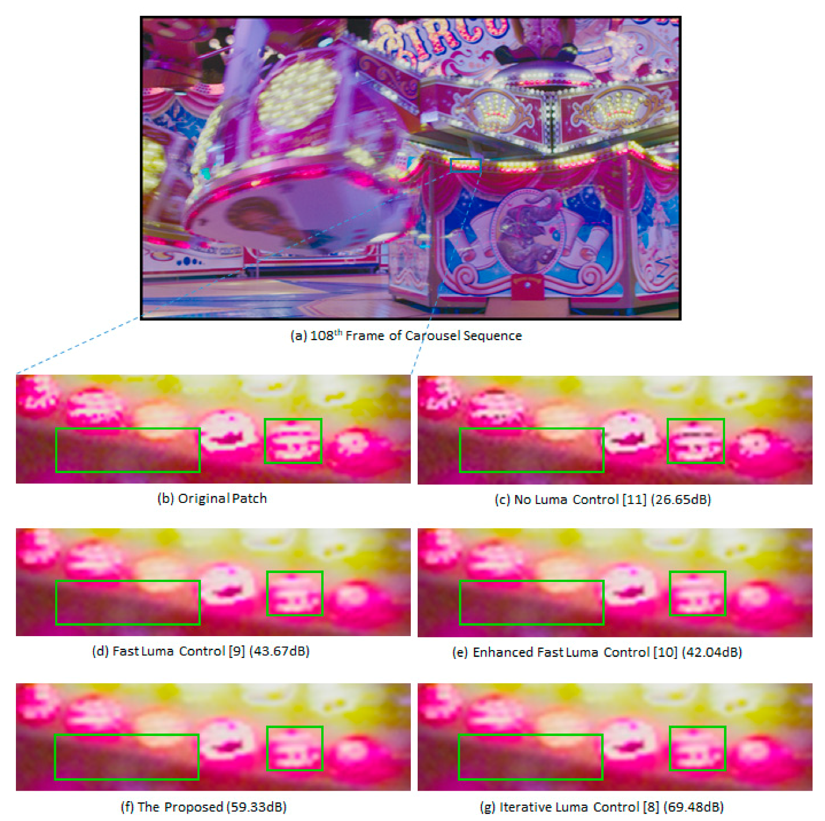
Finally, we show an example of the subjective quality comparison among the tested luma control algorithms. As noted earlier in [5,8,9,10], the artifacts introduced by the NCL Y’CbCr 4:2:0 format would appear as false contours around the object boundary and/or speckle noises in the smooth area. These artifacts become significant in a bright region of highly saturated colors and/or an edge region having large brightness changes. Hence, those artifacts can be easily seen from bright yellow, cyan, or magenta color regions rather than neutral color regions with low-to-medium brightness. Figure 5 shows such artifacts and the quality enhancement by luma control algorithms for the 108th frame of the test sequence “Carousel”, where we highlighted the differences in two parts (see green boxes) of the cropped image patch (i.e., as shown in Figure 5a) among different luma control algorithms. The subfigures b,c of the Figure 5 clearly show the subjective quality problem in the 4:2:0 media format of HDR/WCG video. We can observe that the texture inside the left green box became rougher and the bright pink dots in the right green box got dark after 4:2:0 conversion without luma control. Because of such big changes in brightness, the quality became only 26.65 dB in tPSNR-Y, as shown in Figure 5c. On the other hand, from the subfigures d–g of Figure 5, we can identify that the luma control schemes significantly ameliorate such quality problems and enhance the subjective quality. The rough texture and the dark pink dots disappeared in all luma control outputs, resulting in a better perception of the scene brightness. However, the problematic pink dots are observed to be not fully recovered and the rough textures look smoother than the original, illustrating that a video format with higher chroma resolution is desirable for better perception of HDR/WCG video.

Although the tPSNR-Y values of the subfigures d–g are quite different (i.e., from the 42.04 dB of the “Enhanced Fast Luma Control” scheme in (e) to the 69.48 dB of the “Iterative Luma Control” scheme in (g)), it is hard to observe any subjective difference among the luma control schemes. In order to identify which part was attributed to such a big difference of tPSNR-Y values, we compared the luminance error defined in (1) for the outputs of the 108th frame of “Carousel” sequence produced by the fast and the proposed luma control schemes. After subtracting the per-pixel error of the proposed output from the fast luma control error, we sorted the difference to find the pixel location having high error difference. Then, we marked top 0.1% location with “Green” pixels and cropped the same area as that which was compared in Figure 5. Figure 6 shows the area of the biggest quality difference between the two luma control schemes. We can observe that the green pixels are mostly concentrated on the boundary area showing big brightness changes. Although these differences in a single frame are not clearly perceived as subjectively different in Figure 5, the perturbations of this type of error in consecutive video frames may yield small flicker artifacts in such a boundary area, which can be very annoying to viewers. More examples of the subjective quality comparison can be found in Appendix A of this paper.

5. Conclusions

As a promising type of emerging immersive media, HDR/WCG is starting to replace the main stream of content production for providing far better quality ultra-high definition (UHD) media. The media format, known as HDR10 or HDR10+, has been adopted in various fields of media industry but has possible degradation on luminance perception. Luma control is a method to cope with such potential luminance perception problems and is perceived to be an essential preprocessing technology in HDR/WCG content production. In this paper, we proposed a fast and reliable luma control scheme that can significantly ameliorate the luminance perception error of HDR10/10+ format video and is highly suitable for hardware implementations.

The proposed algorithm employs a linear approximation of EOTF using a straight line passing two points on the EOTF curve, where one is from the original signal and the other from a lower and an upper bound of the optimal luma value. This new linear approximation is the first contribution of this paper. Further, for a more accurate and robust approximation capability of the proposed straight line, we derived two new bounds on the true optimal value based on the solution using truncated Taylor series. This is the second contribution of this paper. Then, in order to demonstrate the feasibility of the proposed luma control scheme, we conducted an extensive comparison study among the previous representative luma control algorithms. Based on the contributions mentioned above, the proposed linear approximation has been identified to provide nearly the same quality of the optimal solution, i.e., only 0.04 dB less than the iterative luma control scheme, in tPSNR-Y on average. Moreover, nearly the same quality was obtained without iteration, resulting in a friendlier nature for hardware implementations. The proposed algorithm showed an impressive quality improvement over the previous fast luma control schemes, i.e., up to 7.4 dB in tPSNR-Y over the fast luma control scheme on the “Fireplace” sequence and up to 3.6 dB over the enhanced fast luma control algorithm on the “Market” sequence. Again, this quality improvement was obtained without any adaptive parameters, which were the required cost for the quality enhancement of the enhanced fast luma control scheme over the fast luma control algorithm.

With these desirable features, the proposed scheme is expected to be highly useful for a practical production system of high-quality HDR/WCG video and to be more valuable due to tighter and more computation-efficient bounds on the optimal luma value.

References

- International Telecommunicaton Union-Radiocommunication sector (ITU-R). Image Parameter Values for High Dynamic Range Television for Use in Production and International Programme Exchange; Rec. ITU-R BT.2100; ITU-R: Geneva, Switzerland, 2016. [Google Scholar]
- Society of Motion Picture and Television Engineers (SMPTE). High Dynamic Range Electro-Optical Transfer Function of Mastering Reference Displays; ST 2084; SMPTE: White Plains, NY, USA, 2014. [Google Scholar]
- Digital Entertainment Content Ecosystem (DECE) LLC. Common File Format & Media Formats Specification, version 2.1; DECE: Beaverton, OR, USA, 2015. [Google Scholar]
- Stessen, J.; Nijland, R.; Brondjik, R.; Grois, R. Chromaticity Based Color Signals for Wide Color Gamut and High Dynamic Range; ISO/IEC doc. m35065; Moving Picture Experts Group (MPEG): Strasbourg, France, 2014. [Google Scholar]
- Strom, J. Investigation of HDR Color Subsampling; ISO/IEC doc. m35841; Moving Picture Experts Group (MPEG): Geneva, Switzerland, 2015. [Google Scholar]
- Chung, K.-L.; Huang, Y.-H.; Lin, C.-H. Improved universal chroma 4:2:2 subsampling for color filter array video coding in HEVC. Signal Image Video Process. 2017, 11, 1041–1048. [Google Scholar] [CrossRef]
- Chung, K.-L.; Hsu, T.-C.; Huang, C.-C. Joint chroma subsampling and distortion-minimization based luma modification for RGB color images with application. IEEE Trans. Image Process. 2017, 26, 4626–4638. [Google Scholar] [CrossRef] [PubMed]
- Strom, J.; Samuelsson, J.; Dovstam, K. Luma adjustment for high dynamic range video. In Proceedings of the IEEE Data Compression Conference (DCC), Snowbird, UT, USA, 29 March–1 April 2016. [Google Scholar]
- Norkin, A. Fast algorithm for HDR color conversion. In Proceedings of the IEEE Data Compression Conference (DCC), Snowbird, UT, USA, 29 March–1 April 2016. [Google Scholar]
- Oh, K.-S.; Kim, Y.-G. Enhanced fast luma adjustment for high dynamic range television broadcasting. J. Broadcast Eng. 2018, 23, 302–315. [Google Scholar]
- Sharma, G.; Wu, W.; Dalal, E.N. The CIEDE2000 Color-Difference Formula: Implementation Notes, Supplementary Test Data, and Mathematical Observations. Color Res. Appl. 2004, 30, 21–30. [Google Scholar] [CrossRef]
- International Organization for Standardization/International Electrotechnical Commission (ISO/IEC). Conversion and Coding Practice for HDR/WCG Y’CbCr 4:2:0 Video with PQ Transfer Characteristics; ISO/IEC doc. N16505; ISO/IEC: New York, NY, USA, 2016. [Google Scholar]
- International Telecommunicaton Union-Radiocommunication sector (ITU-R). Parameter Values for the HDTV Standards for Production and International Programme Exchange; Rec. ITU-R BT.709-6; ITU-R: Geneva, Switzerland, 2015. [Google Scholar]
- International Telecommunicaton Union-Radiocommunication sector (ITU-R). Parameter Values for Ultra-High Definition Television Systems for Production and International Programme Exchange; Rec. ITU-R BT.2020-2; ITU-R: Geneva, Switzerland, 2015. [Google Scholar]
- International Organization for Standardization/International Electrotechnical Commission (ISO/IEC). Call for Evidence (CfE) for HDR and WCG Video Coding; ISO/IEC doc. N15083; ISO/IEC: New York, NY, USA, 2015. [Google Scholar]
- Froehlich, J.; Grandinetti, S.; Eberhardt, B.; Walter, S.; Schilling, A.; Brendel, H. Creating cinematic wide gamut HDR-video for the evaluation of tone mapping operators and HDR-displays. Proc. SPIE 2014, 9023. [Google Scholar] [CrossRef]
Figure 1.
Conventional preprocessing stages for high dynamic range and wide color gamut (HDR/WCG) video in [12].
Figure 2.
A linear approximation of the electro-optical transfer function (EOTF) and the quantities in (14).
Figure 3.
Representative images for selected HDR/WCG test sequences.
Figure 4.
The enhancement results of different luma control algorithms in terms of tPSNR-Y in (a) and tPSNR-XYZ in (b). The number inside the brackets in the “E-Fast” row of (a) denotes the reduction factor, r, in (12), which was employed for the best result for each test sequence.
Figure 5.
The visual effect comparison for the test sequence “Carousel” (108th frame). The number in parentheses for each subfigure means the tPSNR-Y value of the image patch produced by each luma control algorithm.
Figure 6.
Top 0.1% pixels having the biggest quality difference between the proposed and the fast luma control schemes. The green pixels attributed most to the tPSNR-Y difference between the two luma control schemes.