A Mixed Property-Based Automatic Shadow Detection Approach for VHR Multispectral Remote Sensing Images

Abstract

Shadows in very high-resolution multispectral remote sensing images hinder many applications, such as change detection, target recognition, and image classification. Though a wide variety of significant research has explored shadow detection, shadow pixels are still more or less omitted and are wrongly confused with vegetation pixels in some cases. In this study, to further manage the problems of shadow omission and vegetation misclassification, a mixed property-based shadow index is developed for detecting shadows in very high-resolution multispectral remote sensing images based on the difference of the hue component and the intensity component between shadows and nonshadows, and the difference of the reflectivity of the red band and the near infrared band between shadows and vegetation cover in nonshadows. Then, the final shadow mask is achieved, with an optimal threshold automatically obtained from the index image histogram. To validate the effectiveness of our approach for shadow detection, three test images are selected from the multispectral WorldView-3 images of Rio de Janeiro, Brazil, and are tested with our method. When compared with other investigated standard shadow detection methods, the resulting images produced by our method deliver a higher average overall accuracy (95.02%) and a better visual sense. The highly accurate data show the efficacy and stability of the proposed approach in appropriately detecting shadows and correctly classifying shadow pixels against the vegetation pixels for very high-resolution multispectral remote sensing images.

1. Introduction

With the development of aerospace techniques, an increasing number of very high-resolution (VHR) satellites have been launched in recent years, such as Ikonos, QuickBird, Pleiades, GeoEye, RapidEye, Skysat-1, WorldView-2, WorldView-3, Jilin-1, and Kompsat [1,2,3,4,5,6,7,8,9,10]. The VHR multispectral remote sensing images captured by these satellites can depict more details of typical land cover, including buildings, vegetation and roads. Along with the improvement in the optical spatial resolution, shadow interference in these multispectral remote sensing images has become more serious. Obviously, shadow analysis is more important than ever before for these VHR multispectral remote sensing image applications. Shadow occurs when ground objects are illuminated by the sun or other light sources. Additional clues can be obtained through analyzing the related shadows, which provide information about the position of the light source as well as the shape and the structure of ground objects. Since shadows in VHR multispectral remote sensing images indicate additional information about ground objects, shadows may supply useful information for applications such as buildings reconstruction and height evaluation [11,12]. Notably, shadows always result in loss and distortion of land cover within shadow regions, because shadow regions always present low radiance and different spectral reflectivity properties from nonshadow areas [3,13,14,15,16,17]. However, objects in shadow regions may contain significant information, especially in VHR multispectral remote sensing images. Given this situation, detecting shadows effectively plays a role in the analysis of VHR multispectral remote sensing images. Besides, though a wide range of research has explored shadow detection, shadow pixels are still more or less omitted and wrongly confused with vegetation pixels in some cases, and these traditional shadow detection methods are usually aimed at detecting shadows in middle resolution remote sensing images rather than in VHR multispectral remote sensing images [11,12,13,14,18,19,20]. Therefore, well-performed shadow detection approaches for VHR multispectral remote sensing images are necessary for effectively detecting shadows especially targeted at further managing problems of shadow omission and vegetation misclassification.

During recent decades, an increasing number of shadow detection approaches have been developed for analyzing remote sensing images. In general, the related works on shadow detection are usually categorized into either model-based or property-based methods. The model-based methods require prior knowledge about the scene, the sun, and sensors, such as the geometry of the scene, solar elevation and azimuth, the altitude and acquisition parameters of sensors, etc. [21,22,23,24]. Though the model-based technique usually presents desirable performance in shadow detection in specific applications, it is limited by the unavailability of some required prior information. The shortcomings of the model-based methods mentioned above are effectively overcome with the latter method. The property-based methods identify shadows with shadow characteristics, such as spectral features and geometrical information. Due to its accuracy and simplicity, the property-based methods are being widely explored in the literature [11,18,19,24,25,26,27,28,29].

In the property-based group, a certain shadow index image is first generated—in most related works—which usually exploits functions of multispectral bands either directly or indirectly based on the analysis of multispectral remote sensing images. Then, the index image is thresholded by some automatic threshold methods, after which the resulting shadow image is presented. Many researchers at home and abroad have made efforts in these two aspects, attempting to either develop new shadow image indexes, or modify or present improved thresholding methods for better detecting shadows in multispectral remote sensing images. Many researchers indirectly exploited the functions of multispectral bands by using luminance and chromaticity in various invariant color spaces to detect shadows, including hue-intensity-saturation (HIS), hue-saturation-value (HSV), luma-inphase-quadrature (YIQ), YCbCr and C1C2C3 models. Tsai [11] presented an automatic property-based shadow detection approach, which attempted to solve problems caused by cast shadows in color aerial images in complex urban environments. A spectral ratio index (SRI) was developed in this approach to highlight shadow pixels based on the properties of shadow regions compared with nonshadow ones in invariant color spaces, as seen in the hue-intensity-saturation (HIS), hue-saturation-value (HSV), luma-inphase-quadrature (YIQ), and YCbCr invariant color spaces. Then, the final shadow image was obtained by thresholding the index image with the Otsu threshold method [30]. This shadow detection algorithm accurately identifies shadow pixels otherwise bluish and greenish objects present. On the foundation of Tsai’s work, Chung et al. [29] proposed a novel successive thresholding scheme (STS), instead of the global thresholding method used in Tsai’s approach, for more accurately detecting shadows. The STS-based shadow detection algorithm has comparable shadow detection accuracy to Tsai’s SRI-based method. Khekade and Bhoyar [12] also presented an extended spectral ratio index (ESRI) approach based on Tsai’s work [11], in which the SRI-based method was extended with post-processing procedures specifically in the YIQ invariant color space. This ESRI-based method obtained a better visual sense at the expense of longer computational time than Tsai’s SRI-based method without post processing procedures.

Ma et al. [18] introduced a normalized saturation-value difference index (NSVDI) in the HSV invariant color space to detect shadows in high-resolution multispectral remote sensing images. The NSVDI-based method generated a rough shadow index image, highlighting shadows by exploiting the properties of higher saturation and lower intensity of shadows compared with those of nonshadows. The rough shadow index image was then manually thresholded with a certain threshold value to provide a final shadow image. This NSVDI-based method performs well in detecting large shadows in high-resolution multispectral remote sensing images despite omitting some building shadows and small shadows. Additionally, Sarabandi et al. [31] developed a novel method for detecting cast shadow boundaries in high-resolution remote sensing images, in which a C3 index was exploited to highlight shadows. The C3 index is a transformation of red, green and blue bands in the C1C2C3 invariant color space [32]. This C3-based method is able to discriminate shadows from other dark land cover. Based on the work of Sarabandi et al., Besheer et al. [20] presented a modified C3 (MC3) index, in which a near infrared band was added. This MC3-based approach improves the shadow detection results in contrast to the C3-based method introduced by Sarabandi et al. [31].

Several researchers have developed new shadow detection indices based on the analysis of the spectral differences between shadow pixels and typical land cover pixels by directly using multispectral bands, including both the visible bands (red, green, and blue bands) and the near infrared band. In 2015, Chen et al. [14] introduced a new shadow detection method combining the spectral reflectivity characteristics of shadow regions in multispectral bands (i.e., the visible bands and the near infrared band), and the typical normalized difference vegetation index (NDVI). In this method, a normalized blue-red index (NBRI) was originally put forward. Then, the difference in the NBRI and the NDVI was calculated as the final shadow intensity (SI). The SI-based method presents good shadow detection performance for high-resolution multispectral remote sensing images, especially for the WorldView-2 multispectral images, except for wrongly identifying vegetation pixels as shadow ones in some cases. In the next year, Li et al. [24] presented a novel method that joined model and observation cues: pixels values, chromaticity, and luminance. A shadow mask in an image was first outlined with an improved bright channel prior (BCP), which was developed based on the original BCP. Then, the shadow mask was refined by combining the shadow mask with observation cues. This method is suitable not only for remote sensing images but also natural images. In 2017, Mostafa et al. [19] proposed a new shadow detector index (SDI) for detecting shadows in high-resolution multispectral remote sensing images, especially aimed at accurately classifying shadow pixels from vegetation pixels. This SDI-based method was developed by analyzing the difference in shadow pixels and vegetation pixels in nonshadows in terms of green and blue bands, as well as low red values in shadow pixels. An SDI index image was first obtained. Then a shadow image was generated by applying an optimal threshold over the rough index image, in which the optimal threshold was automatically achieved from the SDI histogram with the modified neighborhood valley-emphasis threshold method (NVETM) [33]. This SDI-based approach performs well in classifying shadow pixels from vegetation pixels, and achieves high shadow detection accuracies, except for the shortcomings of omitting some small shadow areas and misclassifying some dull red roof pixels as shadow pixels. Wang et al. [23] proposed a simple and automatic shadow detection method. In this method, a shadow mask was achieved by delineating shadow and nonshadow regions in the VHR image with a geometric model of the scene and the solar position. Then, the shadow mask was refined by applying a matting method to the image. This method performed well for detecting fine shadows and shadows within water regions. However, some small shadow areas were ignored in the detecting shadow process. Besides, the geometrical information for the scene and the solar position is usually unavailable, and two-step shadow detection is time-consuming. For efficiency and simplicity, the reviewed shadow detection algorithms [11,14,18,19,20] are selected for comparing algorithm performance with that of our proposed shadow detection approach.

In this paper, a mixed property-based shadow index (MPSI) is developed for detecting shadows in VHR multispectral remote sensing images, especially to further address the problem where true shadow areas are more or less omitted and vegetation cover types in nonshadow areas are usually wrongly classified as shadows to somewhat. This developed approach employs the difference in properties between shadows and nonshadows with respect to the chromaticity (specifically for the hue component) and the luminance (namely, the intensity component) in HSV invariant color space, and the reflectivity difference properties between shadow regions and vegetation cover in nonshadows in terms of multispectral bands (visible bands and near infrared band). Based on these properties, rough shadow images are first obtained. Then, final shadow images are generated with an optimal threshold on the rough shadow images.

The rest of the paper proceeds as follows. Property analysis and the proposed shadow detection approach are described in Section 2. Section 3 presents the experimental conditions and comparative experiment results on three test images of the multispectral WorldView-3 remote sensing images of Rio de Janeiro, Brazil in comparison with five standard shadow detection algorithms [11,14,18,19,20]. After that, these comparative experiment results are discussed in Section 4. Finally, conclusions are drawn in Section 5.

2. Materials and Methods

In our research, we devoted ourselves to exploring a new and effective shadow detection method for accurately identifying shadows in VHR multispectral remote sensing images, especially for further mitigating the shadow detection problems of shadow omission and vegetation misclassification. For this purpose, we explored properties of shadow regions in terms of the chromaticity (the hue component) and luminance (the intensity component) in the HSV invariant color space, as well as the spectral properties of both shadow areas and vegetation cover in nonshadow areas with respect to the reflectivity of multispectral bands (visible bands and near infrared band). Then, based on the property study, we developed a new shadow detection index employing both the chromaticity and luminance properties in shadow and nonshadow regions, and the reflectivity characteristics of multispectral bands (visible bands and near infrared band) for both shadow regions and vegetation cover in nonshadow areas. Finally, a shadow image was achieved by automatically applying an optimal threshold obtained over the index image. In this section, we briefly state the property analysis, and present the proposed shadow detection procedure in detail.

2.1. Property Analysis

In this part, we describe our study with respect to two types of properties of shadow regions. For the first one, invariant color properties are explored in the HSV invariant color space in terms of chromaticity (specifically hue component) and luminance (intensity component). For the other one, multi-spectral bands are engaged in analyzing features of shadow pixels and the vegetation pixels within nonshadow areas.

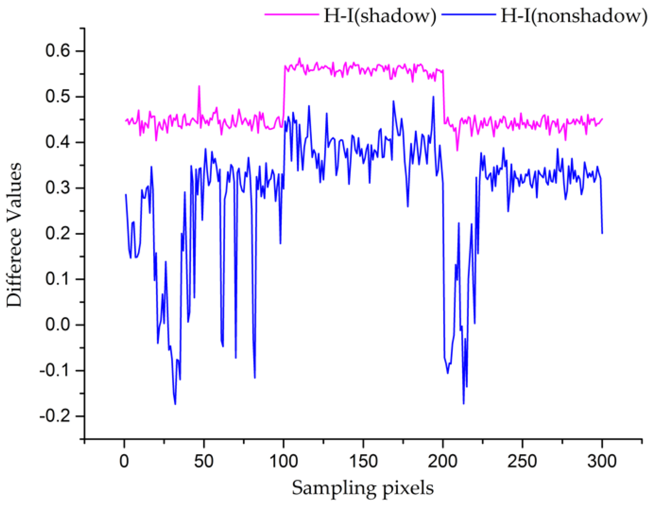
2.1.1. Analysis of Chromaticity and Luminance

We, as humans, are easily able to differentiate shadows from nonshadows according to the sensation perceived directly from digital images, due to the two classes of receptors in our eyes: cones and rods [34]. However, for the same application in detecting shadows, computer programs usually encounter various problems, such as illumination variation, atmospheric effect, and boundary ambiguity [11]. Additionally, in automatic shadow detection applications with computer programs, luminance and chromaticity are powerful descriptors for color images, including multispectral remote sensing images. Generally, chromaticity consists of hue and saturation, and luminance is also called intensity. In particular, hue is a significant attribute associated with the dominant wavelength in the mixture of light waves, which is taken together with saturation as the chromaticity, in which saturation refers to the relative purity of a certain color. Luminance is the most powerful descriptor for color images [18,34]. Regarding the powerful performance of chromaticity and luminance in describing features of color images, we were inspired to determine whether we could specifically employ characteristics of shadows within multispectral remote sensing images in terms of chromaticity and luminance. Consequently, we explored properties of shadow pixels in comparison with those of the corresponding nonshadow pixels in the HSV invariant color space, which performs well in separating chromaticity and luminance composites.

Theoretically, according to the Phong’s illumination model [35] and the imaging model of Huang et al. [26], the light illuminating a small patch of a certain surface includes three parts: the ambient part, the diffusion part and the specular part. In most practical applications, the specular part can be neglected, because land cover in forests and urban areas is usually matte and dull. With respect to the ambient and diffusion parts of the incident light, nonshadow areas are always lighted by both the ambient and the diffusion part; however, shadow areas are almost always only illuminated by the ambient part rather than both.

Therefore, shadow regions are able to be differentiated from nonshadows in accordance with whether or not the diffusion part of incident light exists. Accordingly, reflectivity of the diffusion part of the incident light expresses the difference between shadow and nonshadow regions, and the difference is [32,36]:

$$C_d=m_d{\displaystyle {\int }_{\lambda }{f}_c(\lambda )e(\lambda )c_d(\lambda )d\lambda }$$

(1)

where $C_d\in \left\{R_d,G_d,B_d\right\}$ provides the red, green, and blue sensor response to the diffusion part of the incident light, $m_d$ is independent of the wavelength $\lambda$ and only depends on the geometry information, $f_c(\lambda )\in \left\{f_R(\lambda ),f_G(\lambda ),f_B(\lambda )\right\}$ denotes the spectral sensitivity in function of wavelength $\lambda$, $e(\lambda )$ is the quantity of incident light, and $c_d(\lambda )\in \left\{R_d(\lambda ),G_d(\lambda ),B_d(\lambda )\right\}$ is the surface albedo in terms of the red, green, and blue bands, respectively.

On the other hand, in remote sensing applications, the sun is always considered to be the sole incident light source, and its illumination can be regarded as white illumination in which the quantity of incident light $e(\lambda )$ equals to a certain constant that is no longer related to the wavelength $\lambda$ as before. Under this situation, the integrated white condition [32,37] holds, as shown in Equation (2):

$${\displaystyle {\int }_{\lambda }{f}_c(\lambda )d\lambda }=k$$

(2)

where $k$ is approximately equal to a certain constant.

According to electromagnetic wave theory, the surface albedo is positively proportional to the wavelength $\lambda$, namely the surface albedo $c_d\left(\lambda \right)$ of the near infrared (NIR) is larger than that of the red (R), the surface albedo of R is larger than that of the green (G), and the surface albedo of G is larger than that of the blue (B). Thus, the decreasing response of the near infrared, red, green and blue sensor to shadow areas against the corresponding nonshadow areas follow the inequation relationship shown in Equation (3):

$$NI{R}_d>R_d>G_d>B_d$$

(3)

where $NI{R}_d$, $R_d$, $G_d$, and $B_d$ are the surface albedo in terms of the near infrared (NIR), red (R), green (G), and blue (B) bands, respectively.

Meanwhile, both the hue component of chromaticity and the intensity component of luminance are functions of R, G, and B in RGB color space, as shown in Equations (4) and (5) [26,37]:

$$I=\frac{1}{3}(R+G+B)$$

(4)

$$H={\tan }^{-1}\left(\frac{\sqrt{3}(G-B)}{(R-G)+(R-B)}\right)$$

(5)

where $I$ and $H$ denote the intensity and hue components, respectively, and $R$, $G$, and $B$ are reflectivity values of the red, green, and blue bands, respectively.

Additionally, Huang et al. calculated the hue value under shadow using [26]:

$$H_{shadow}={\tan }^{-1}\left(\frac{\sqrt{3}(G_{shadow}-B_{shadow})}{(R_{shadow}-G_{shadow})+(R_{shadow}-B_{shadow})}\right)$$

(6)

where $H_{shadow}$, $R_{shadow}$, $G_{shadow}$, and $B_{shadow}$ are hue, red, green, and blue values of shadow regions, respectively.

According to the analysis of the difference in illumination of shadow and nonshadow regions, the hue value $H_{shadow}$ under shadow conditions can be converted into the format corresponding to that under nonshadow conditions, as shown in Equation (7):

$$H_{shadow}={\tan }^{-1}\left(\frac{\sqrt{3}\left((G-G_d)-(B-B_d)\right)}{\left((R-R_d)-(G-G_d)\right)+\left((R-R_d)-(B-B_d)\right)}\right)$$

(7)

where $R$, $G$, and $B$ denote reflectivity values of the red, green and blue bands of nonshadow regions, respectively, and $R_d$, $G_d$, and $B_d$ are the reflectivity values of the diffusion part of the incident light in terms of the red, green, and blue bands, respectively.

Consequently, a conclusion is drawn that the hue value H_shadow of shadow regions is usually higher than that of nonshadow areas based on Equation (3) [26]:

$$H_{shadow}>H_{nonshadow}$$

(8)

where $H_{shadow}$ and $H_{nonshadow}$ are the hue values of shadow and nonshadow regions, respectively.

Apart from the hue value, the intensity value of shadow regions can be obtained using Equation (9):

$$\begin{array}{l}{I}_{shadow}=\frac{1}{3}\left(R_{shadow}+G_{shadow}+B_{shadow}\right)\\ =\frac{1}{3}\left((R-R_d)+(G-G_d)+(B-B_d)\right)\\ =I-\frac{1}{3}\left(R_d+G_d+B_d\right)\end{array}$$

(9)

where $I_{shadow}$ is the intensity value of the shadow regions, $R$, $G$, and $B$ denote reflectivity values of the red, green and blue bands of nonshadow regions, respectively, and $R_d$, $G_d$, and $B_d$ are the reflectivity values of the diffusion part of the incident light in terms of the red, green, and blue bands, respectively. Obviously, the intensity value $I_{shadow}$ of the shadow regions is lower than the intensity $I_{nonshadow}$ of nonshadow areas, as shown in Equation (10).

$$I_{shadow}<I_{nonshadow}$$

(10)

When the hue component and the intensity component are normalized into the range of [0,1], a conclusion can be deduced for the difference values between the hue and the intensity components, i.e.,$H_{shadow}-I_{shadow}$ for shadows and $H_{nonshadow}-I_{nonshadow}$ for nonshadows, as shown in Equation (11), according to the unequal relation of the hue component between shadows and nonshadows shown in Equation (8), and the unequal relation of the intensity component between shadows and nonshadows, shown in Equation (10).

$$H_{shadow}-I_{shadow}>H_{nonshadow}-I_{nonshadow}$$

(11)

Based on the analysis of the difference in illumination on shadow and nonshadow regions, as well as the hue and intensity values of shadow and nonshadow regions mentioned above, the property of shadows can be summarized as follows with respect to the hue and intensity components in the HSV invariant color space in comparison with that of nonshadows:

(1)

Higher hue value due to the reflection quantity of a certain wavelength $\lambda$ is positively proportional to the wavelength $\lambda$ [11,26].

(2)

Lower intensity value due to the direct light from the sun being obstructed, and only the ambient part is illuminating the shadowed areas, rather than both the ambient and the diffusion part of the light source, which are illuminating the nonshadow regions.

(3)

Higher differences between the hue component and the intensity component for shadow regions than those of nonshadow regions.

Accordingly, a sampling procedure was applied over many multispectral WorldView-3 remote sensing images at the pixel level in terms of hue and intensity components for both shadow and nonshadow areas. The sampling procedure produced a difference curve between the hue component and the intensity component for shadow regions, and a difference curve between the hue component and the intensity component for nonshadow regions, which are plotted together as shown in Figure 1. The sampling curves in Figure 1 verify the theoretical conclusion above, that greater difference values are observed between the hue component and the intensity component in shadow regions compared to the nonshadow regions. Consequently, we employed the characteristics above of the shadow regions in the HSV invariant color space to highlight shadow regions in test images.

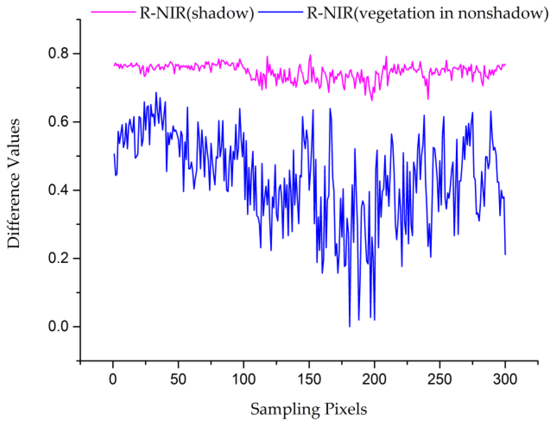
2.1.2. Analysis of Multispectral Bands

In addition to the study of shadow characteristics with respect to the chromaticity (specifically, the hue component) and the luminance (namely, the intensity component) in the HSV invariant color space, we were also inspired by the fact that land cover, especially many kinds of vegetation, present various reflectivity to different wavelengths according to electromagnetic wave theory [38]. Based on this inspiration, we studied important differences between shadow and vegetation areas in terms of the multispectral reflectivity in multispectral bands, namely, visible bands (red, green, and blue bands) and the near infrared band. According to electromagnetic wave theory, when electromagnetic waves with different wavelengths are incident to the same object, the particles composing the object show different reflectivity characteristics to these incident electromagnetic waves of different wavelengths [38,39]. Consequently, various reflectivity values are achieved, meaning reflectivity values of different land cover types vary in accordance with the wavelengths of the incident electromagnetic waves. Specifically, the visible bands consist of electromagnetic waves with wavelengths ranging around 445 to 749 nm (i.e., ranges of 445 to 517 nm, 507 to 586 nm, and 626 to 696 nm, for blue, green, and red bands, respectively), and the near infrared band includes electromagnetic waves with wavelengths in the range of about 765 to 1039 nm [40]. Therefore, reflectivity values of a certain land cover usually vary in the red, green, blue and near infrared bands. Additionally, both components and structure of land cover are key factors in the reflectivity for a certain wavelength electromagnetic wave. Due to the components and the special cell structure of vegetation, the reflectivity of the near infrared band is far higher than that of visible bands [38]. Nevertheless, the reflectivity of the red band is obviously the lowest, in comparison with that of the near infrared, green, and blue bands [14]. An unequal relation is presented in Equation (12) for the special reflectivity property of vegetation in terms of the near infrared band and the red band, as described above:

$$NI{R}_{nonshadow-vegetation}>R_{nonshadow-vegetation}$$

(12)

where $NI{R}_{nonshadow-vegetation}$ and $R_{nonshadow-vegetation}$ are reflectivity values of the near infrared band and the red band, respectively, for vegetation cover in nonshadow regions.

According to the analysis of the difference of illumination on shadow and nonshadow regions in Equation (3), an unequal relation can be drawn, as shown in Equation (13), which describes the reflectivity difference of the near infrared band and the red band between shadow regions and vegetation cover in nonshadow regions.

$$NI{R}_{vegetation-in-nonshadow}-NI{R}_{shadow}>R_{vegetation-in-nonshadow}-R_{shadow}$$

(13)

where $NI{R}_{shadow}$ and $R_{shadow}$ are reflectivity values of the near infrared band and the red band for shadow regions, respectively.

Additionally, according to Equation (10), the reflectivity values of both the near infrared band and the red band decrease dramatically for shadow regions compared with that of vegetation cover types in nonshadow regions, as shown in Equation (14).

$$\{\begin{array}{l}NI{R}_{vegetation-in-nonshadow}>NI{R}_{shadow}\\ R_{vegetation-in-nonshadow}>R_{shadow}\end{array}$$

(14)

Based on the above analysis of the reflectivity property of the near infrared band and the red band for both shadow regions and vegetation cover in nonshadow regions, a conclusion can be drawn for the unequal relation of the reflectivity differences between the red band and the near infrared band in shadow regions and vegetation cover in nonshadow regions, as shown in Equation (15).

$$R_{shadow}-NI{R}_{shadow}>R_{vegetation-in-nonshadow}-NI{R}_{vegetation-in-nonshadow}$$

(15)

Experimentally, we applied a sampling procedure to many multispectral WorldView-3 remote sensing images at the pixel level with regard to the reflectivity on multispectral bands for both shadow regions and many vegetation cover types in nonshadow regions. The resulting reflectivity values of the red band and the infrared band are normalized into the range of [0,1], and are then used to draw the resulting difference curves between the reflectivity values of the red band and the infrared band in both shadow regions and vegetation cover types in nonshadow regions as shown in Figure 2. The resulting sampling curves in Figure 2 verify that shadow regions present higher reflectivity difference values between the red band and the near infrared band compared with vegetation cover in nonshadow regions. Therefore, we attempted to use this reflectivity difference between the red band and the near infrared band in differing shadow regions and vegetation cover in nonshadow regions.

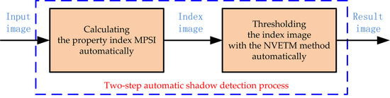
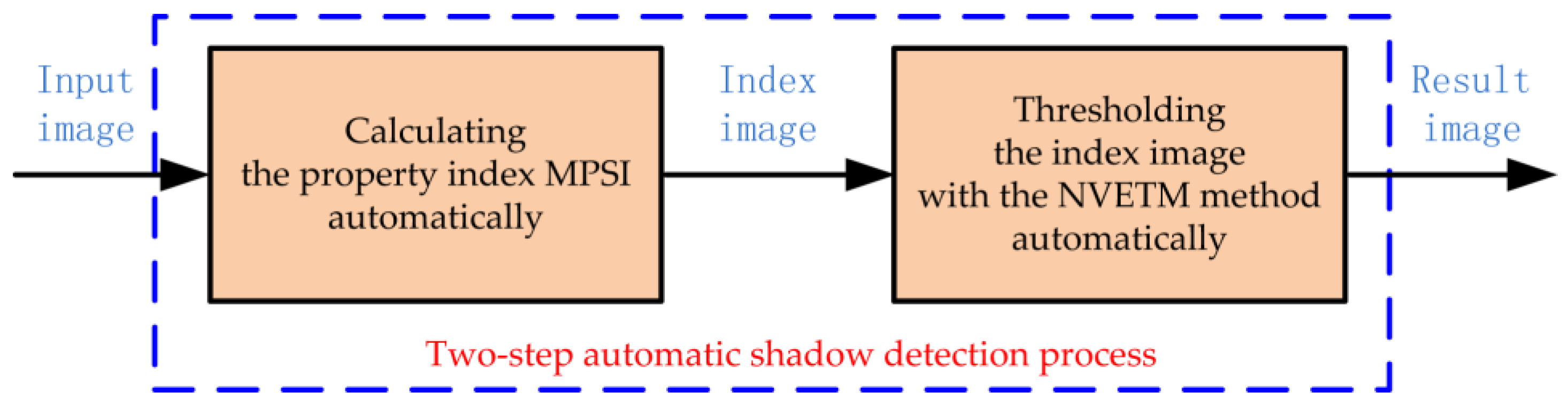
2.2. Proposed Shadow Detection Approach

Based on the study of the properties of the shadow regions with respect to the hue and the intensity components in the HSV invariant color space, as well as in terms the reflectivity of multispectral bands, we proposed a mixed property-based shadow index (MPSI) shown in Equation (16):

$$MPSI=\left(H-I\right)\times \left(R-NIR\right)$$

(16)

where $H$ and $I$ are the normalized values of hue and intensity components, respectively, and $R$ and $NIR$ are normalized reflectivity values of the red band and the near infrared band, respectively.

Due to the properties of the shadow regions in the HSV invariant color space (i.e., higher difference value between the hue component and the intensity component), in this proposed shadow index, we highlighted shadow regions by using the difference of the normalized hue and normalized intensity component, i.e., H − I, to further solve the shadow omission problem. Concurrently, based on the higher reflectivity difference of the red band and the near infrared band for shadow regions in comparison with vegetation cover in nonshadow regions, we used the reflectivity difference of the red band and the near infrared band, i.e., R − NIR, to effectively distinguish shadow regions from vegetation cover in nonshadow regions. From the property analysis mentioned previously, in which both the difference terms H − I and R − NIR in shadows are higher than in nonshadows, we developed a mixed property-based shadow index, as shown in Equation (16), with the product of the difference of the normalized hue and the normalized intensity values, H − I, and the reflectivity difference of the normalized values of the red band and the near infrared band, R − NIR. In principle, the proposed shadow index achieves higher values for shadow pixels when compared with general nonshadows and vegetation cover in nonshadows.

In this paper, we first separated shadow pixels from general nonshadows, as well as vegetation pixels within nonshadow regions, with the developed mixed property-based shadow index (MPSI), from which we draw a shadow index image. Then, we applied a certain threshold technique over the achieved shadow index image to generate the final shadow image automatically which is described in the following section.

2.3. Threshold Method

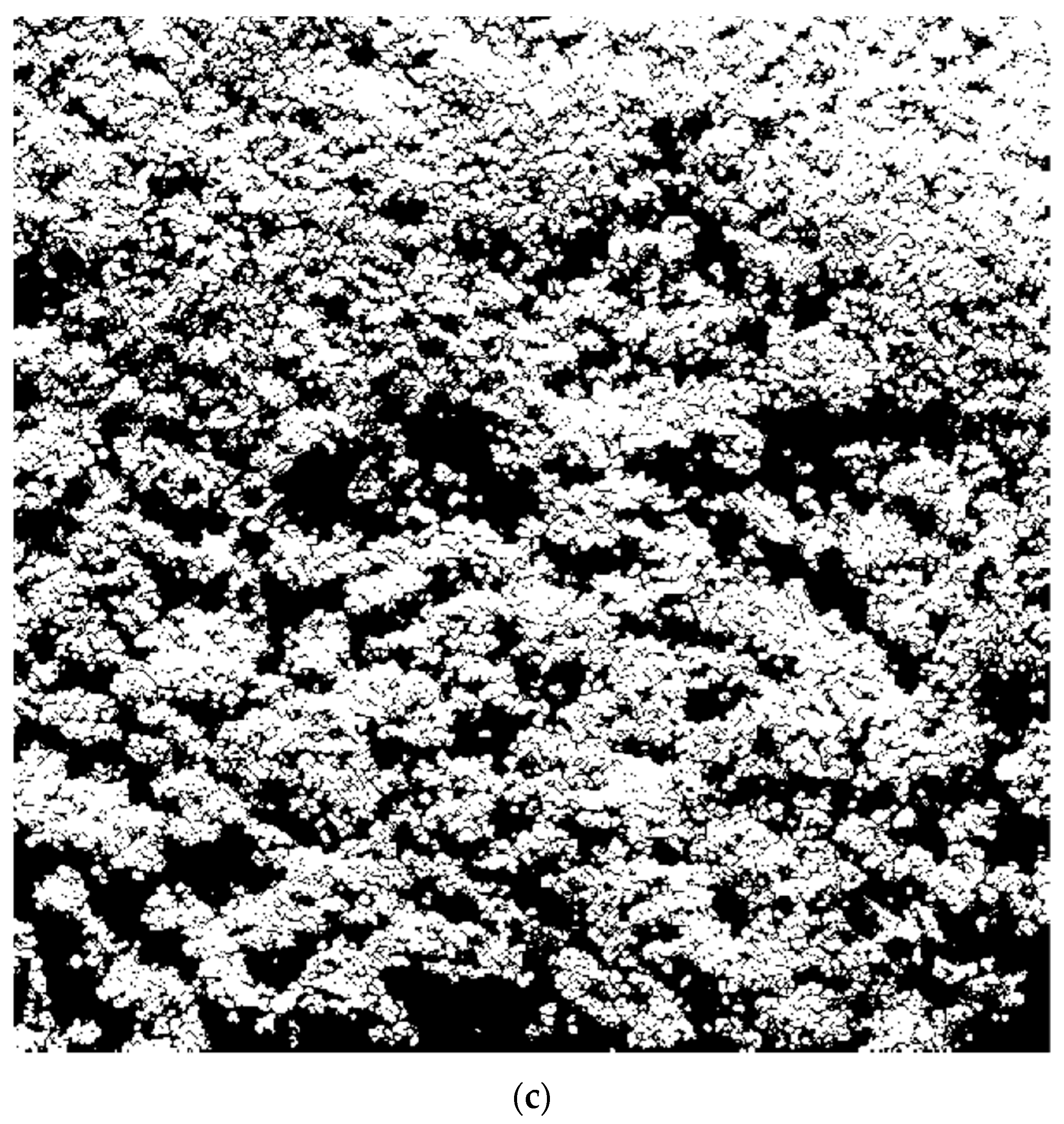
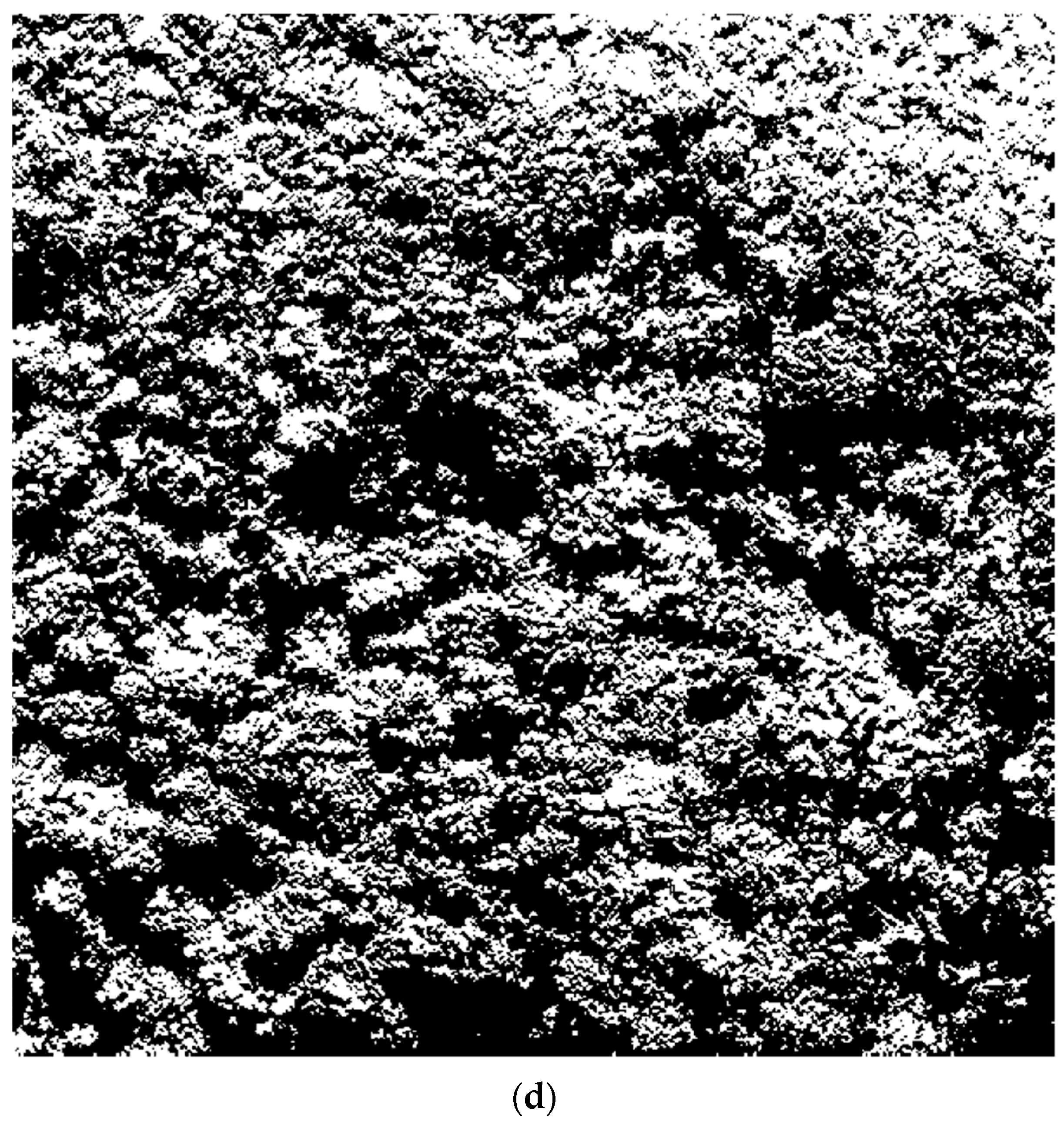
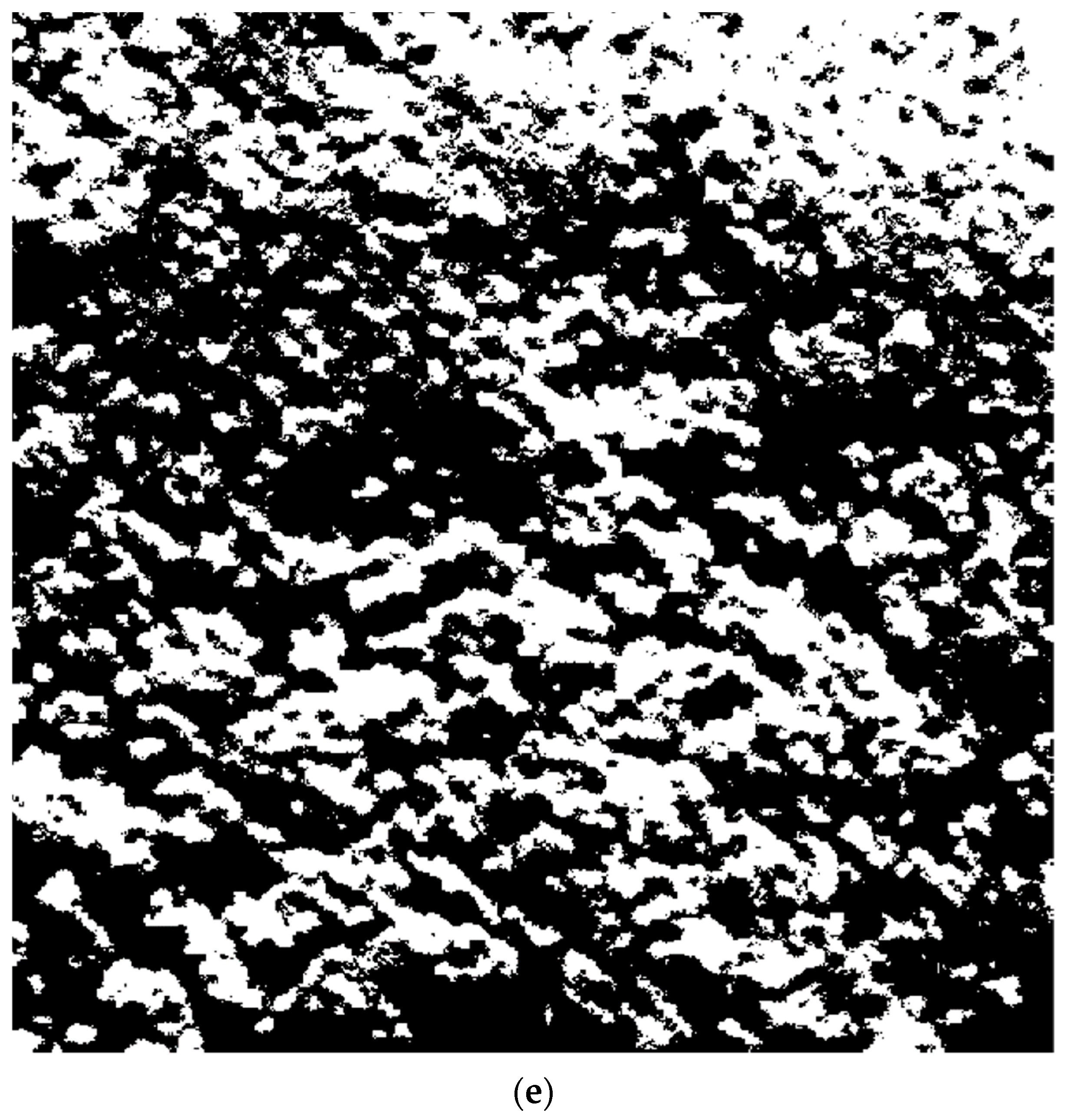
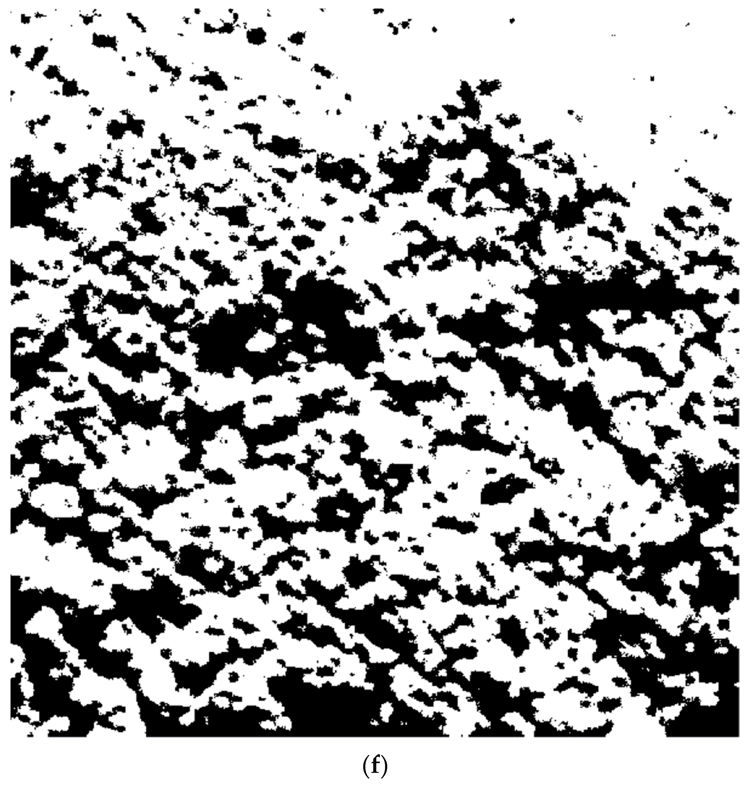
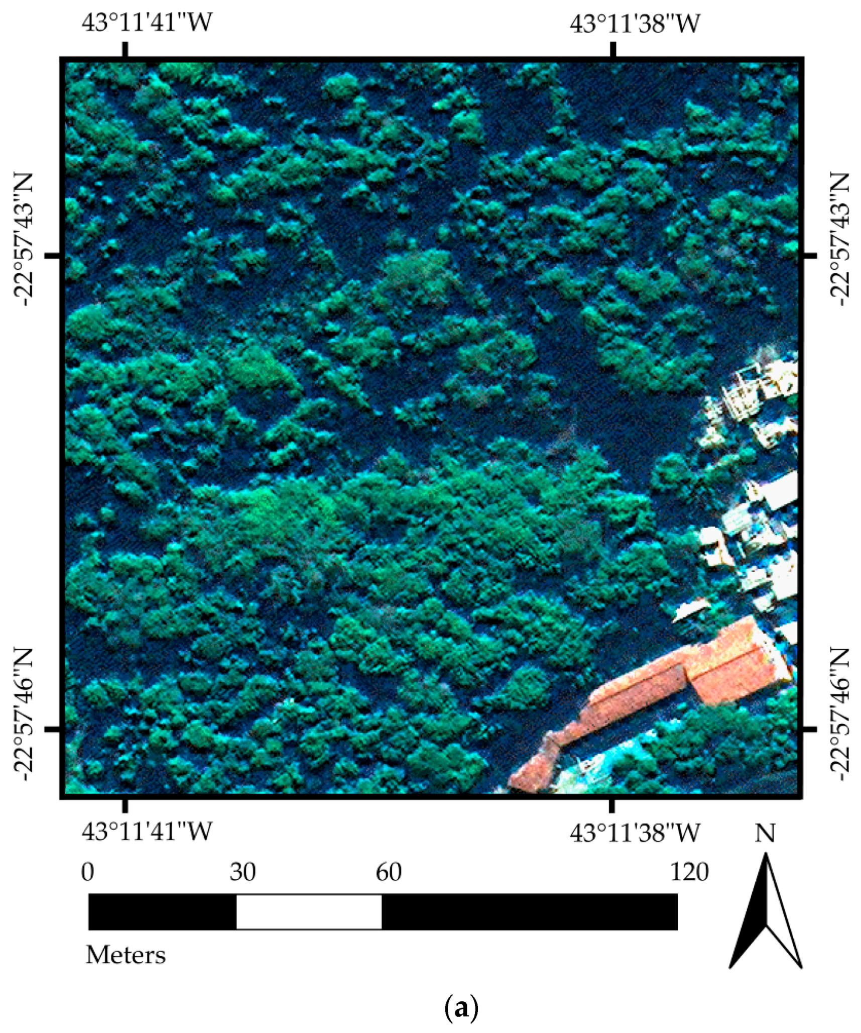
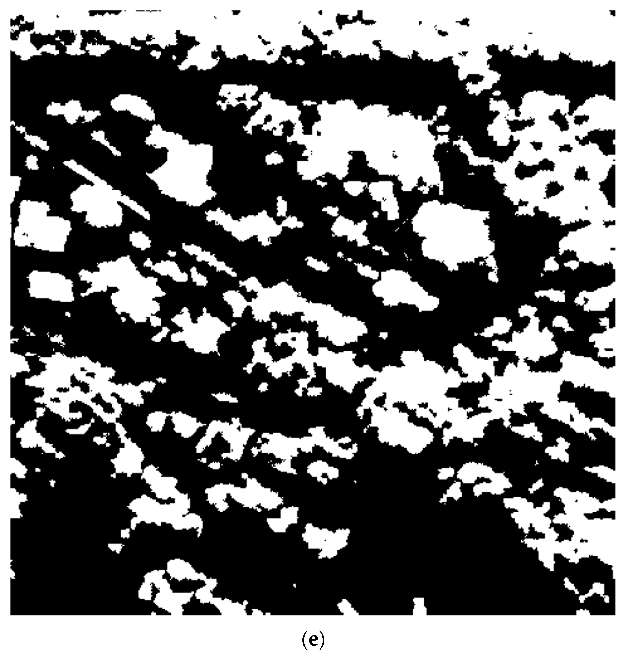
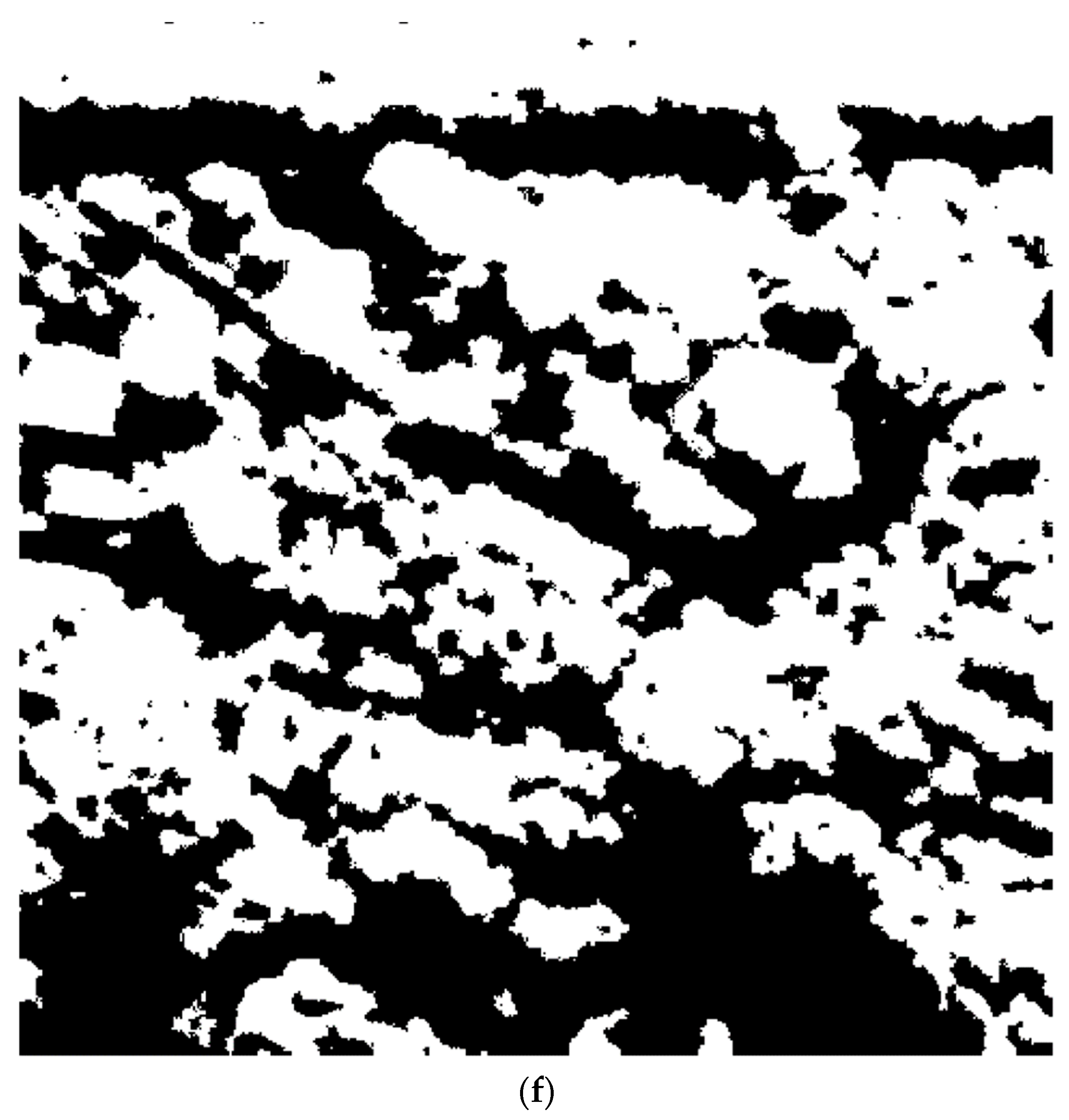
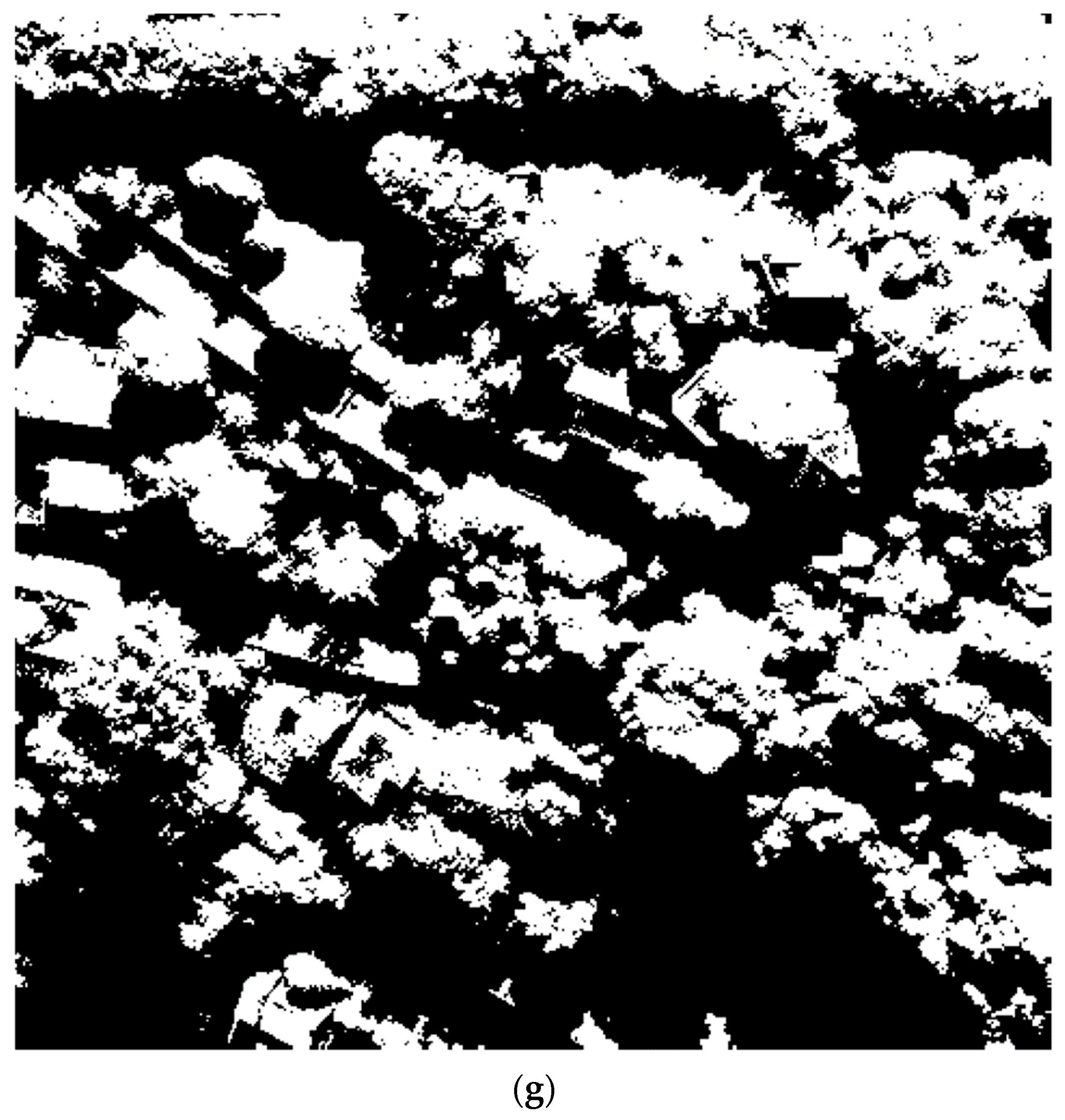
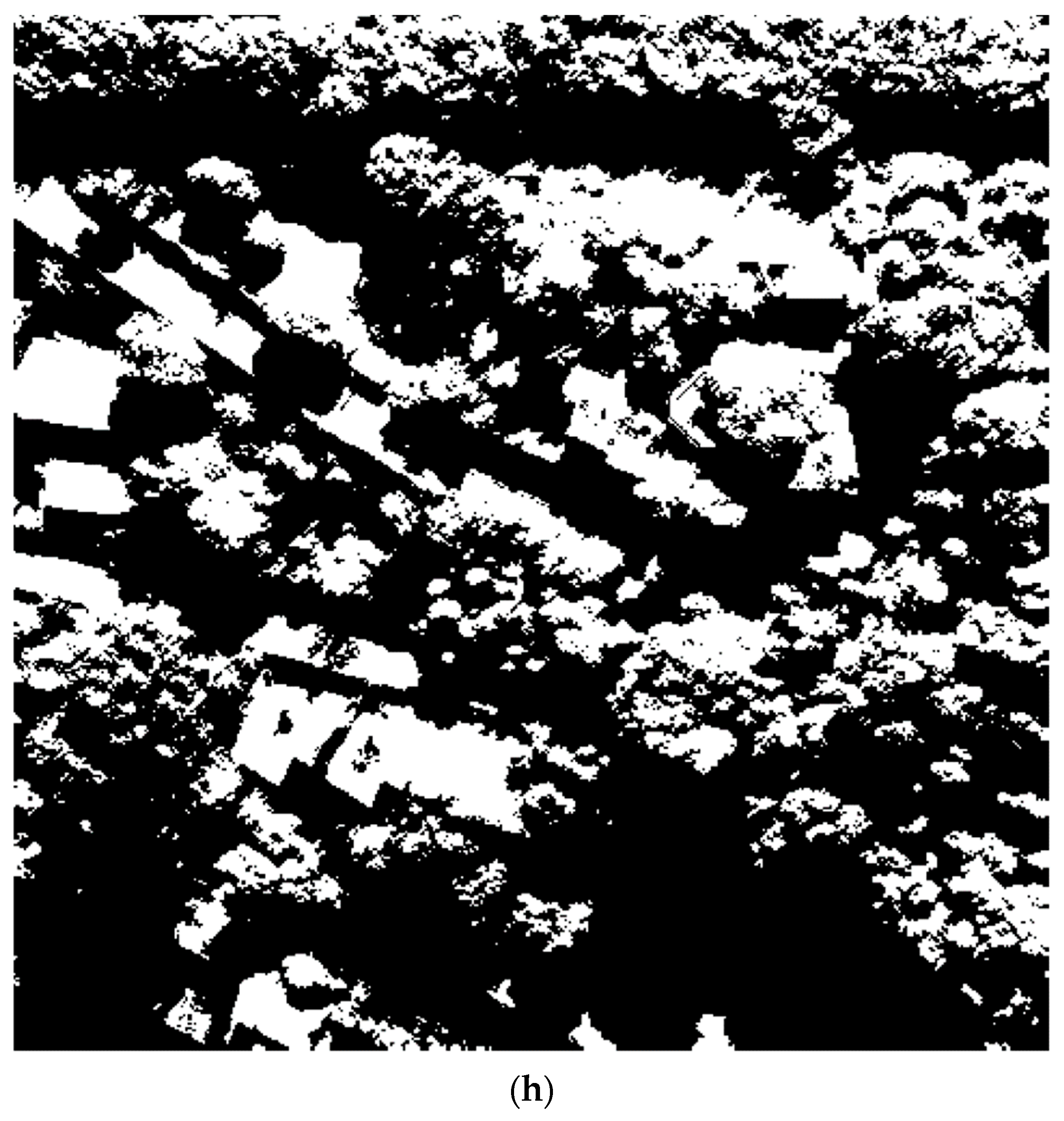
After we obtained the shadow index image with the proposed previously developed mixed property-based shadow index, we applied an optimal threshold to the shadow index image, in which the optimal threshold could be obtained automatically by using several typical threshold methods, such as the Otsu threshold method [30] and the neighborhood valley-emphasis threshold method (NVETM) [33].

Practically, the Otsu threshold method is well known for its simplicity and easy realization, making it one of the typical threshold methods commonly used in practical applications. The Otsu threshold method works well for images of histograms in bimodal distribution or close to bimodal distribution. However, when histograms of the test images are unimodally distributed or close to it, extra measures are needed for the Otsu threshold method to determine an optimal threshold for these images [33]. Furthermore, based on the Otsu method and the previous work of Ng in 2006 [41], Fan et al. developed a new automatic threshold method in 2012, called the neighborhood valley-emphasis threshold method (NVETM). This NVETM has been applied to detecting shadows in high-resolution remote sensing images, and presents satisfactory thresholding results for most images with histograms in either bimodal or unimodal [19]. Therefore, this automatic NVETM was applied in our approach, which was combined with our developed mixed property-based shadow index for detecting shadows in VHR multispectral remote sensing images.

The NVETM is described as follows [33]. First, for gray-level g, the corresponding frequency h(g) is calculated using Equation (17), and the sum of the neighborhood gray probability $\overline{h}(g)$ in interval 2m + 1 is defined as:

$$h(g)=\frac{f(g)}{n},g=0,1,\dots ,L-1$$

(17)

$$\overline{h}(g)={\displaystyle \sum _{i=-m}^{m}h(g+i)}$$

(18)

where $f\left(g\right)$ is the amount of the pixels with gray level $g$, $L$ is the number of gray levels, and $n$ is the number of pixels in the test image.

Then, the test image is binarized into two classes, either 0 or 1, by a predefined threshold $t$, which is computed with Equation (19):

$$\{\begin{array}{l}{p}_0(t)={\displaystyle \sum _{g=0}^{t}h(g)}\\ p_1(t)={\displaystyle \sum _{g=t+1}^{L-1}h(g)}\end{array}$$

(19)

After that, the mathematical expectations of the two classes above are calculated as:

$$\{\begin{array}{l}{\mu }_0(t)=\left[{\displaystyle \sum _{g=0}^{t}gh(g)}\right]/p_0(t)\\ {\mu }_1(t)=\left[{\displaystyle \sum _{g=t+1}^{L-1}gh(g)}\right]/p_1(t)\end{array}$$

(20)

Finally, the NVETM determines an optimal threshold $T$ by maximizing the revised within-class variance $\xi (t)$, as shown in Equation (21):

$$\xi (t)=\left(1-\overline{h}(t)\right)\left[p_0(t){\mu }_0^2(t)+p_1(t){\mu }_1^2(t)\right]$$

(21)

Considering that histogram images may have various distributions, we selected the NVETM by Fan et al. to automatically determine an optimal threshold $T$. With the optimal threshold $T$ obtained above, the shadow image could finally be constructed, combined with our proposed shadow index image by assigning a value of 0 to the pixel with a gray level below the optimal threshold T, and by assigning a value of 1 to that with a gray level above T in the original image, which were regarded as the shadow pixel and the nonshadow pixel, respectively. Figure 3 shows the flow chart of the proposed shadow detection approach.

3. Results

In this section, we describe the experiment conditions and test images used for comparative experiments to demonstrate the performance of our developed shadow detection approach, as well as other comparable shadow detection approaches for different test images, and state the corresponding shadow detection results. These comparative experiments were implemented in MATALAB 2017a under the Microsoft Windows 7 operation system on a DELL personal computer (3.20 GHz CPU and 4 GB RAM).

In these comparative experiments, we tested many multispectral remote sensing images selected from the multispectral WorldView-3 remote sensing image of Rio de Janeiro, Brazil. Given the limitation of paper size, three typical test images (named test image A, B, and C) were selected to validate our MPSI-based shadow detection approach in detecting shadows and correctly distinguishing shadows from vegetation cover of nonshadow areas, as shown in Figure 4. Particularly, four bands in these test images were employed: band-2 (blue), band-3 (green), band-5 (red), and band-7 (near infrared-1). Specifically, test image A in Figure 5a is a 601 × 601 pixel image covering a typical forest scene where various kinds of vegetation are found. Test image B in Figure 6a is a 501 × 501 pixel image with high vegetation coverage and a smaller fraction of buildings. Test image C in Figure 7a is a 481 × 481-pixel image including various land cover types (mainly including vegetation, buildings, roads, and lawns).

Furthermore, to assess our MPSI-based shadow detection approach both subjectively and objectively, we applied our developed shadow detection approach and five comparable methods to test images A, B and C. Results were achieved for these three test images A, B, and C, as shown in Figure 5c–h, Figure 6c–h and Figure 7c–h, respectively, and the accuracy data of the different methods for these three test images were summarized in

Table 1. Shadow detection accuracy data for test image A in Figure 5a.

Method	PA 1 (%)	SP 2 (%)	EO 3 (%)	EC 4 (%)	OA 5 (%)
SRI [11]	75.40	92.98	24.60	7.02	83.28
NSVDI [18]	94.29	81.52	5.71	18.48	88.56
MC3 [20]	86.28	73.06	13.72	26.94	80.35
SI [14]	62.64	97.03	37.36	2.97	78.07
SDI [19]	96.18	86.16	3.82	13.84	91.69
MPSI6	95.78	94.77	4.22	5.23	95.33

¹PA: Producer’s Accuracy; ²SP: Specificity; ³EO: Omitted Error; ⁴EC: Committed Error; ⁵OA: Overall Accuracy; ⁶MPSI: The proposed shadow detection method.

,

Table 2. Shadow detection accuracy data for test image B in Figure 6a.

Method	PA (%)	SP (%)	EO (%)	EC (%)	OA (%)
SRI [11]	97.16	68.75	2.84	31.25	86.94
NSVDI [18]	99.94	11.15	0.06	88.85	68.01
MC3 [20]	79.20	88.52	20.80	11.48	82.55
SI [14]	62.08	93.70	37.92	6.30	73.45
SDI [19]	94.99	90.21	5.01	9.79	93.27
MPSI	95.63	91.76	4.37	8.24	94.24

and

Table 3. Shadow detection accuracy data for test image C in Figure 7a.

Method	PA (%)	SP (%)	EO (%)	EC (%)	OA (%)
SRI [11]	98.88	28.69	1.12	71.31	75.60
NSVDI [18]	99.72	24.87	0.28	75.13	74.89
MC3 [20]	84.52	76.17	15.48	23.83	81.75
SI [14]	64.19	96.94	35.81	3.06	75.06
SDI [19]	86.68	94.45	13.32	5.55	89.26
MPSI	97.19	92.10	2.81	7.90	95.50

, respectively. Additionally, interpretations were carried out manually to generate reference images for these three test images, A, B, and C, as shown in Figure 5b, Figure 6b and Figure 7b, based on these corresponding panchromatic images, respectively. Based on these reference images, several related assessments were carried out both subjectively and objectively to evaluate the performance of our MPSI-based shadow detection approach, which is described in the following section in detail.

Practically, in real-time or approximate real-time shadow detection applications for VHR multispectral remote sensing images, timesaving algorithms draw more attention from most end-users, given equivalent shadow detection results. Therefore, the time consumption is an important metric that is usually considered while designing and selecting shadow detection algorithms.

Table 4. Time consumption of test images A–C shown in Figure 5a, Figure 6a and Figure 7a, respectively.

Time Used (ms)	A	B	C
SRI [11]	89	62	55
NSVDI [18]	60	42	38
MC3 [20]	90	49	56
SI [14]	263	258	277
SDI [19]	276	258	253
MPSI	72	49	47

summarizes the computational time required for detecting shadows in test images A–C, shown in Figure 5a, Figure 6a and Figure 7a, using the proposed MPSI-based shadow detection approach and five other investigated comparable shadow detection algorithms. From the last row of Table 4, the proposed MPSI-based shadow detection approach was verified using a timesaving algorithm. The significant reason for this finding is that the proposed shadow index (MPSI) is very simple.

4. Discussion

In this section, we specifically evaluate the experimental results mentioned above, both subjectively and objectively, based on the comparison of the resulting images shown in Figure 5c–h, Figure 6c–h and Figure 7c–h against the reference images in Figure 5b, Figure 6b and Figure 7b, respectively. We used these assessments to validate the efficacy as well as the shortcomings of our proposal for detecting shadows in VHR multispectral remote sensing images against other available standard shadow detection methods.

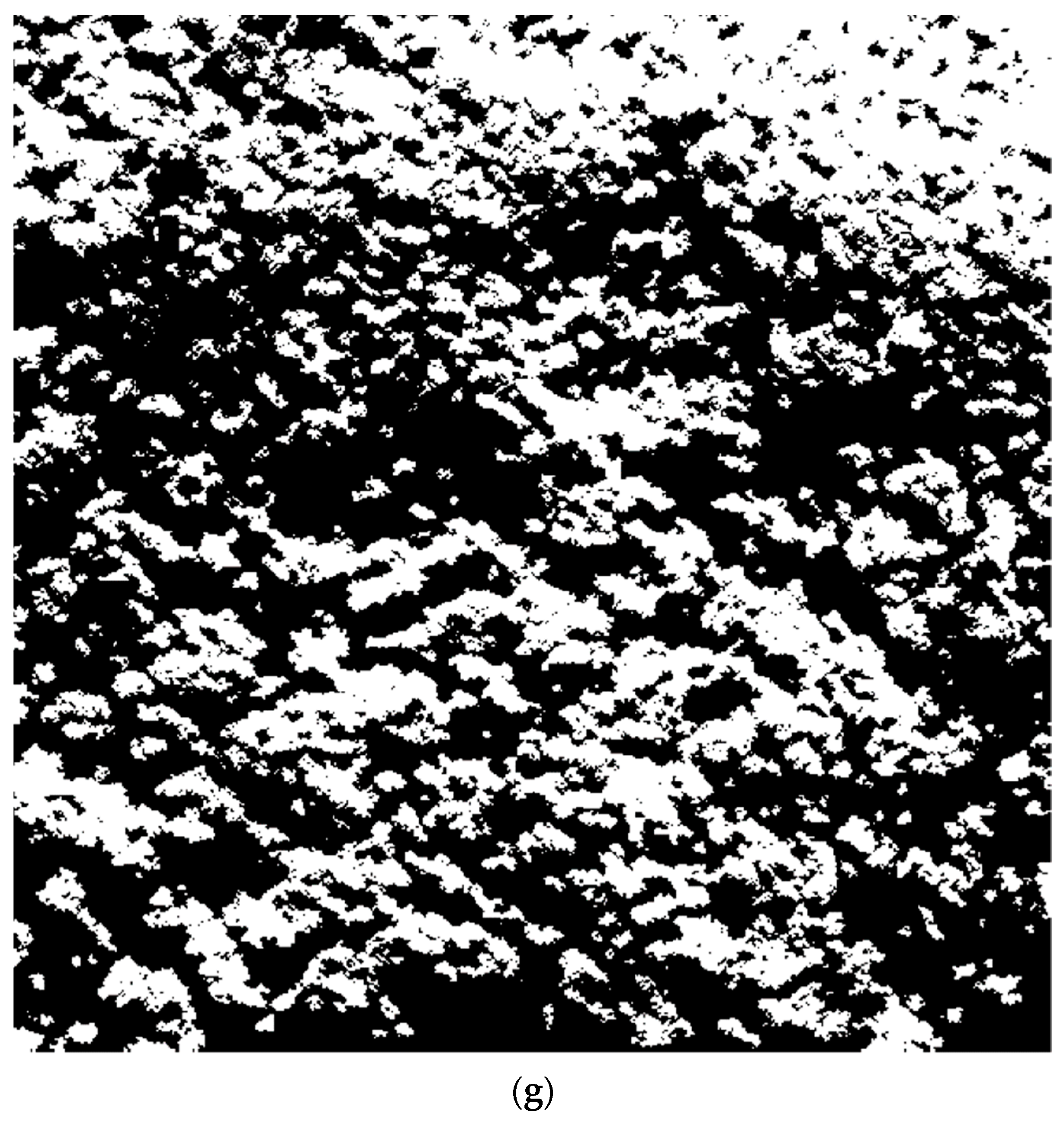
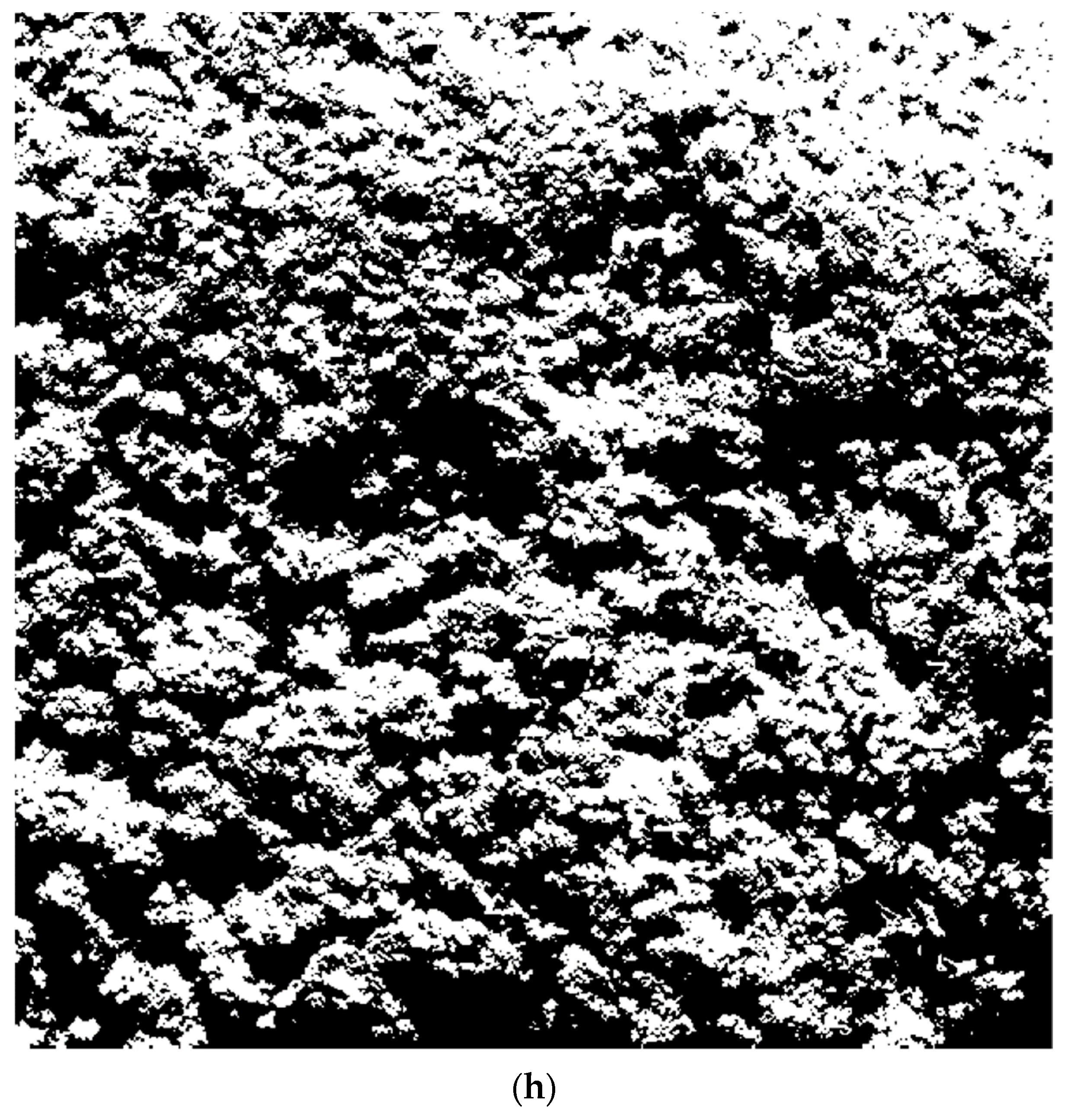
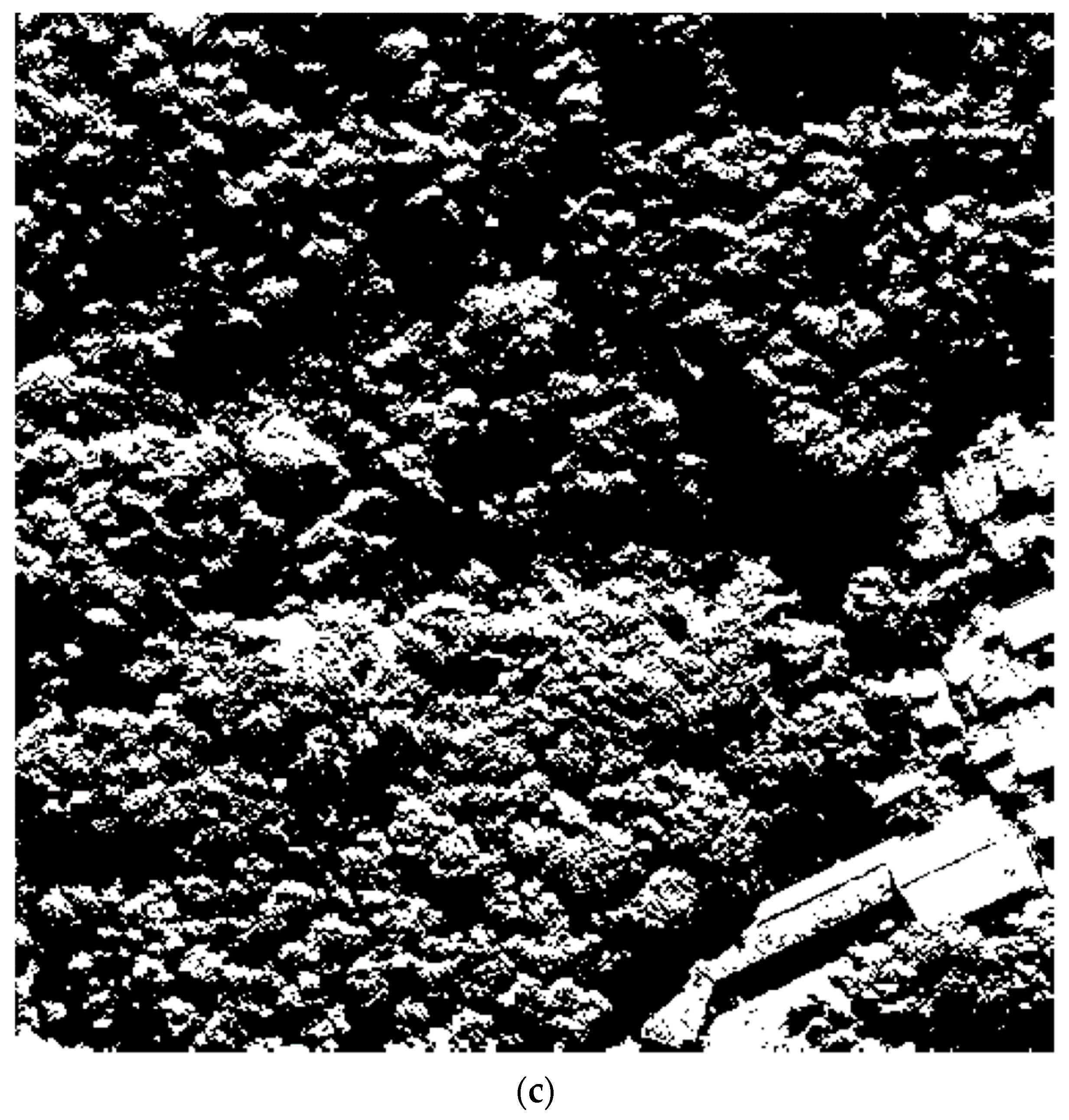
4.1. Subjective Assessment

In this part, we first describe the subjective assessment of the experimental results. Figure 5a, Figure 6a and Figure 7a show these three test multispectral images selected from many tested images of the multispectral WorldView-3 remote sensing image of Rio de Janeiro, Brazil. Figure 5b, Figure 6b and Figure 7b present the corresponding reference images that were manually interpreted from these three test images in panchromatic version respectively. These reference images are regarded as ground-truth images when assessments were applied over the resulting images using various shadow detection methods, such as the SRI-based method in Tsai [11], the NSVDI-based method in Ma et al. [18], the MC3-based method in Besheer et al. [20], the SI-based method in Chen et al. [14], the SDI-based method in Mostafa et al. [19], and our proposed MPSI-based approach. To validate the effectiveness of our proposed approach in resolving the problems of shadow omission and vegetation misclassification, we chose these three test images because they mainly include many small shadow regions and high coverage of vegetation, named test images A, B, and C, as shown in Figure 5a, Figure 6a and Figure 7a, respectively. Assessments of test images A, B, and C are described in detail as follows.

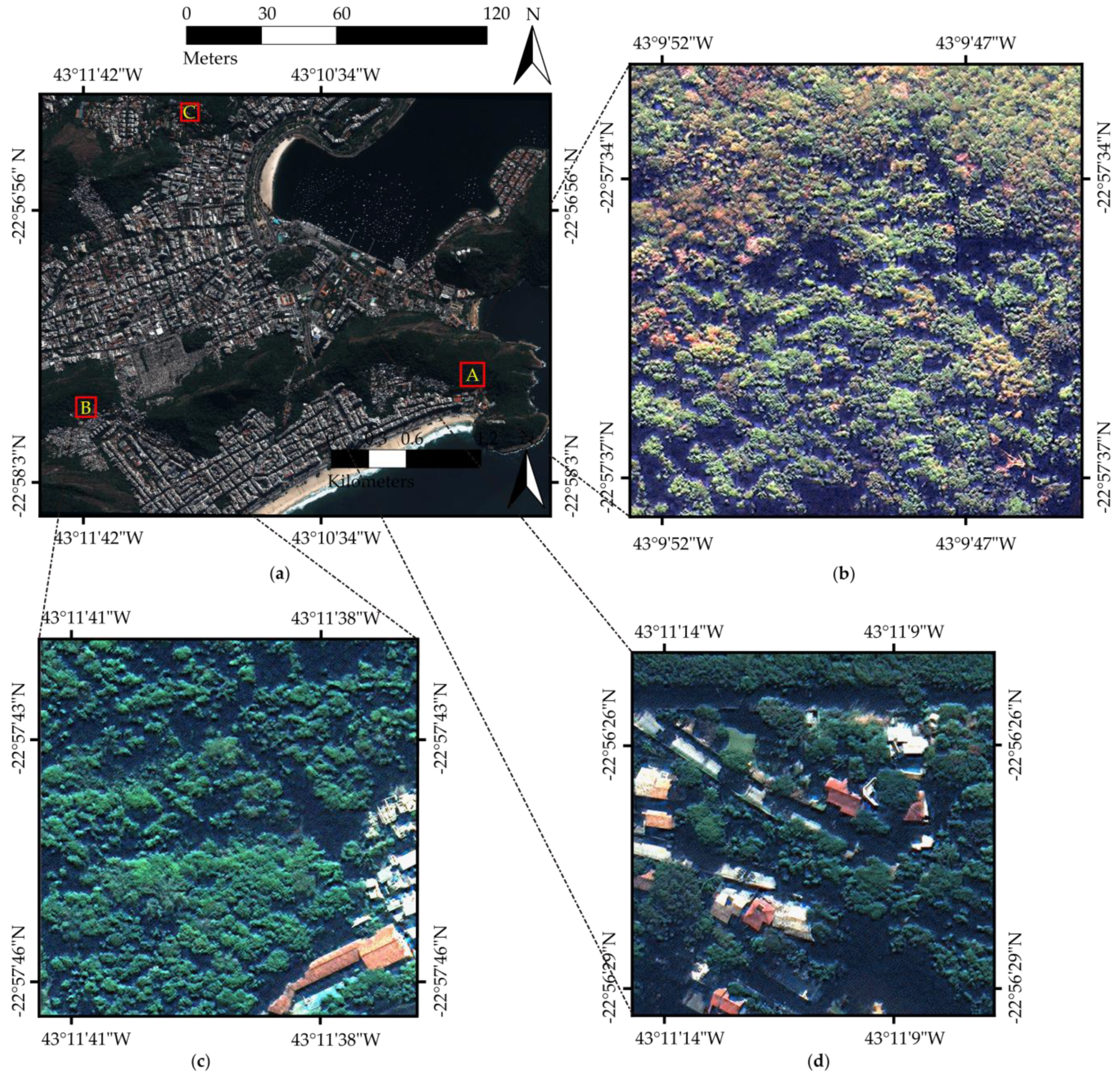
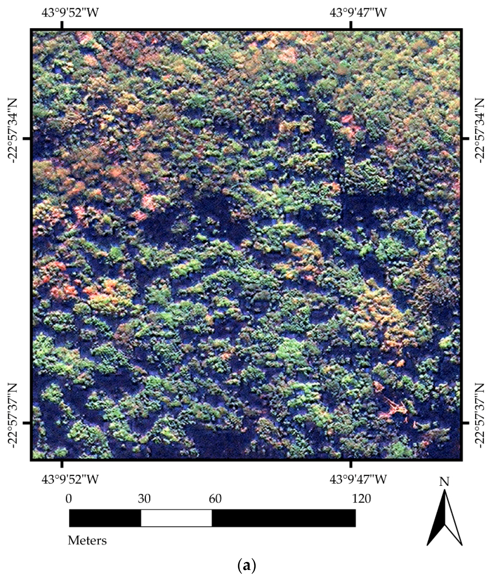
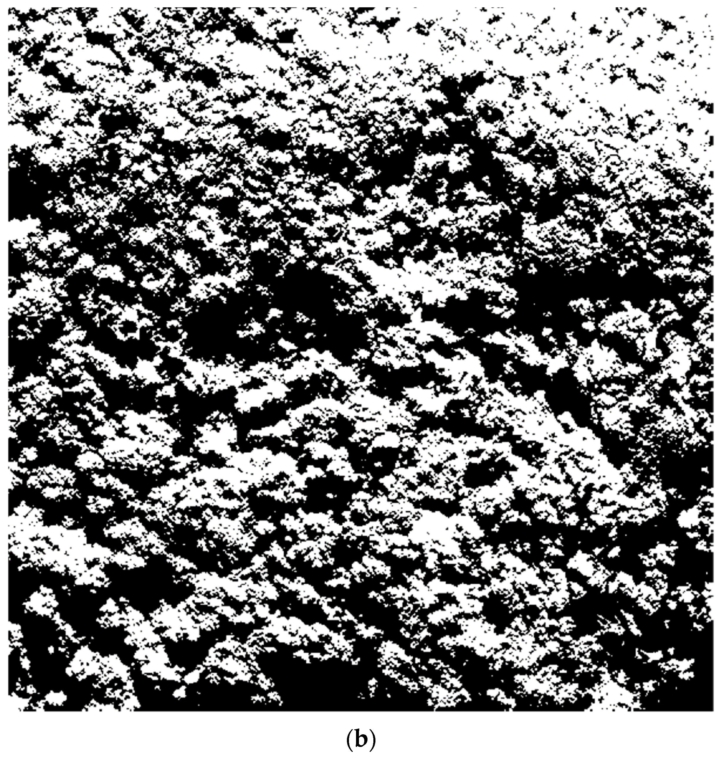
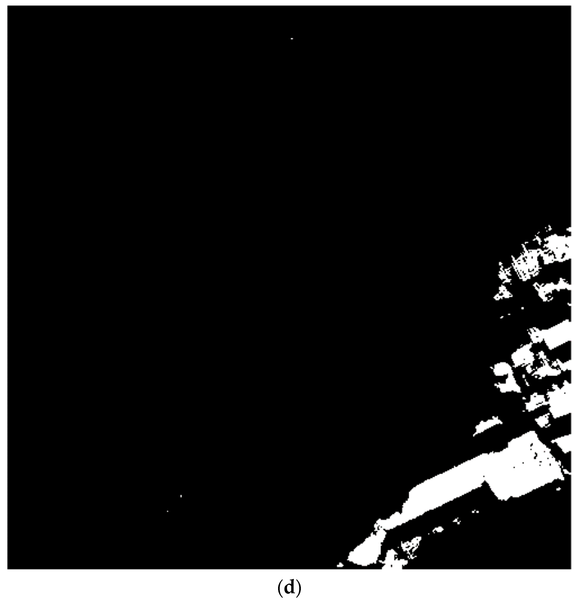
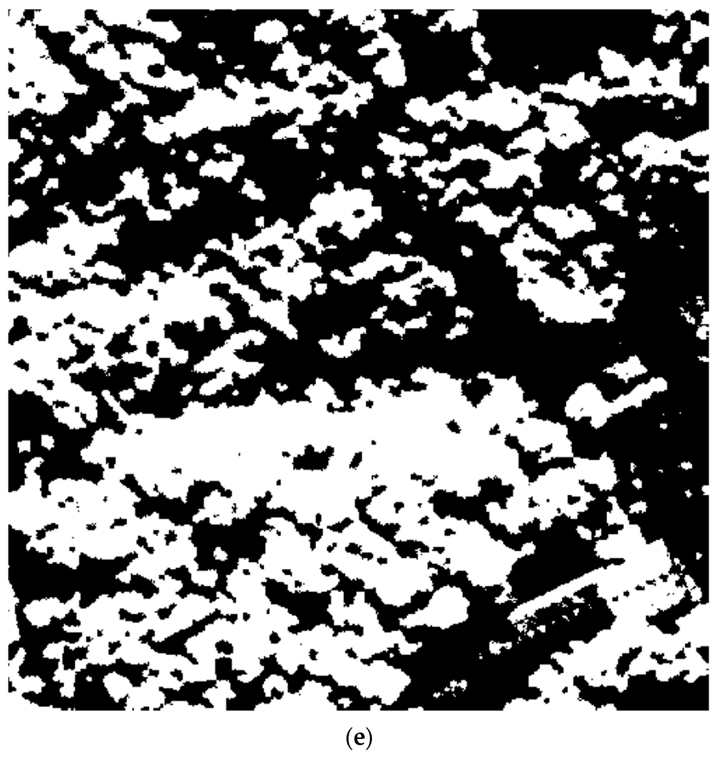
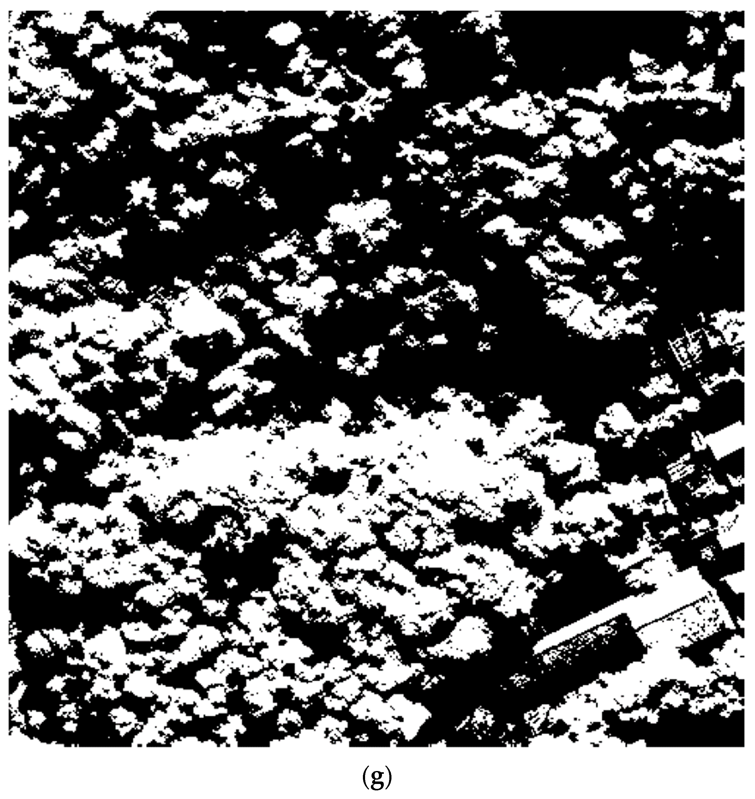
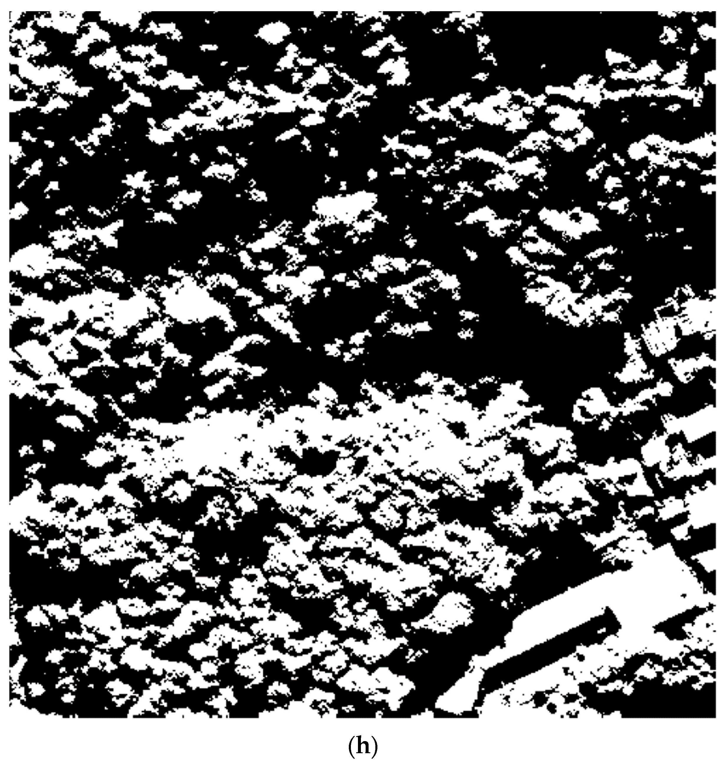
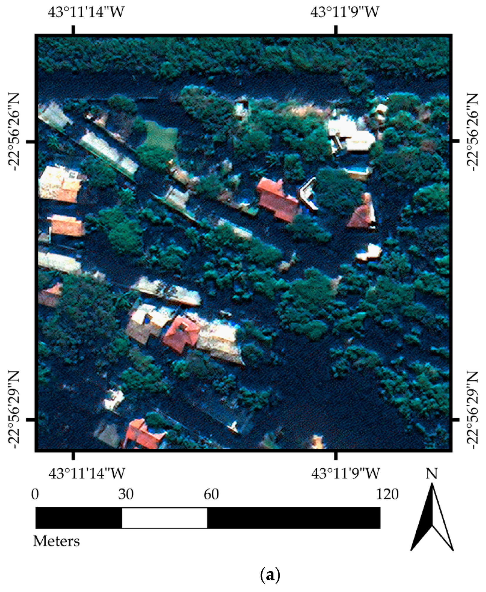
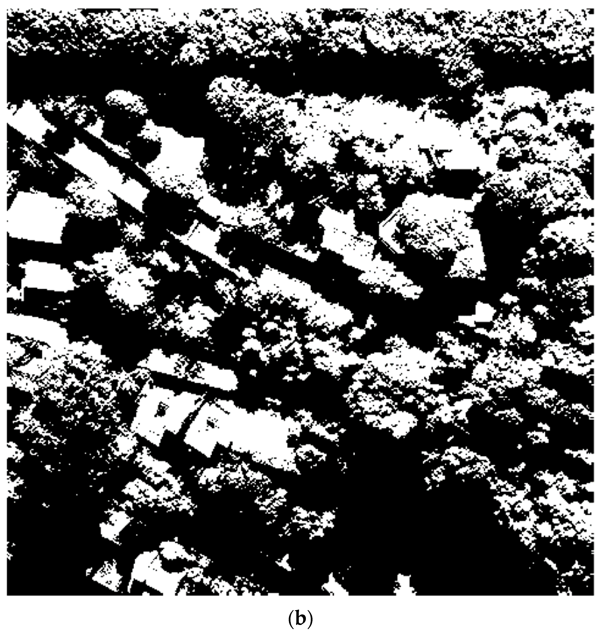
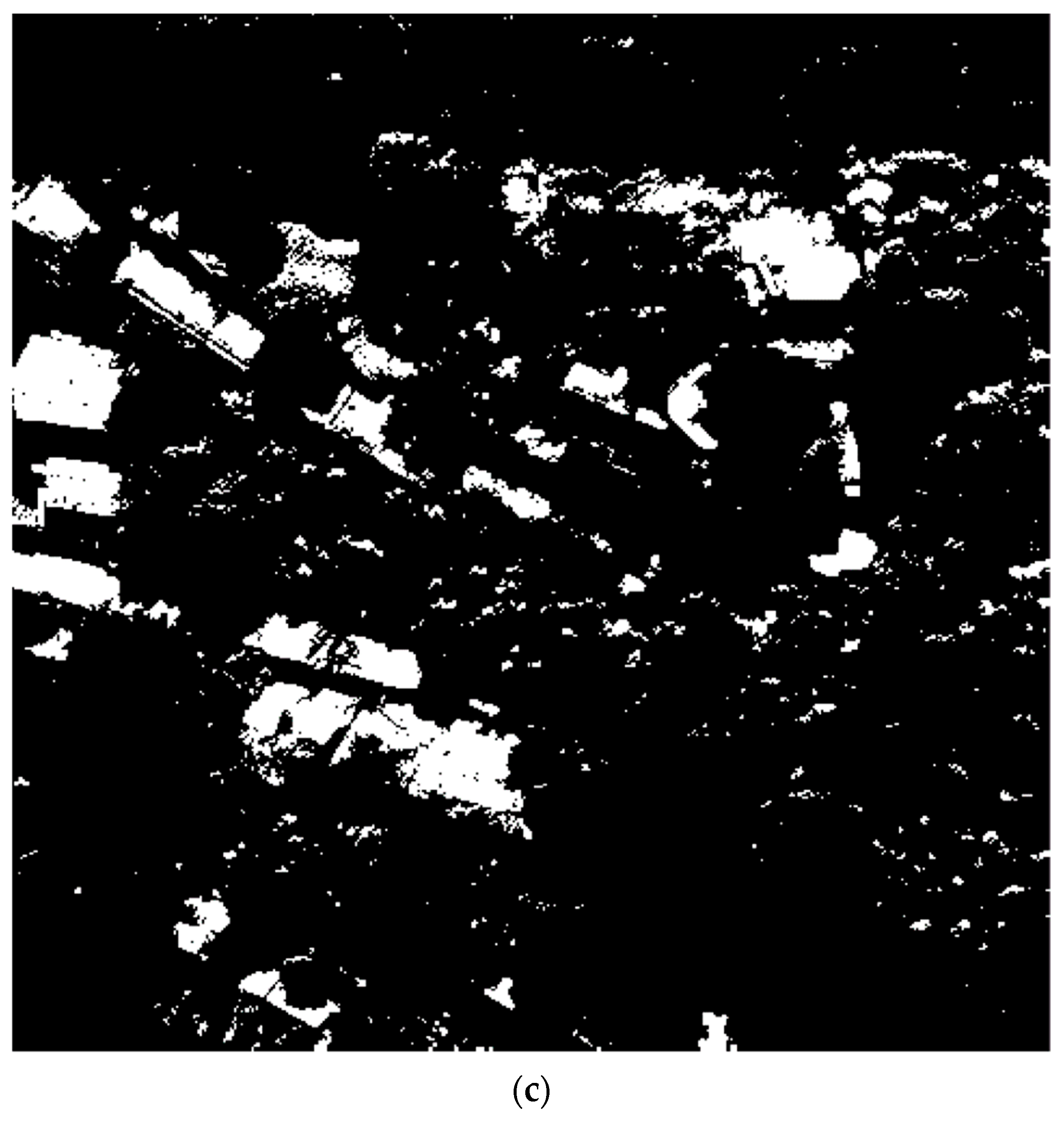
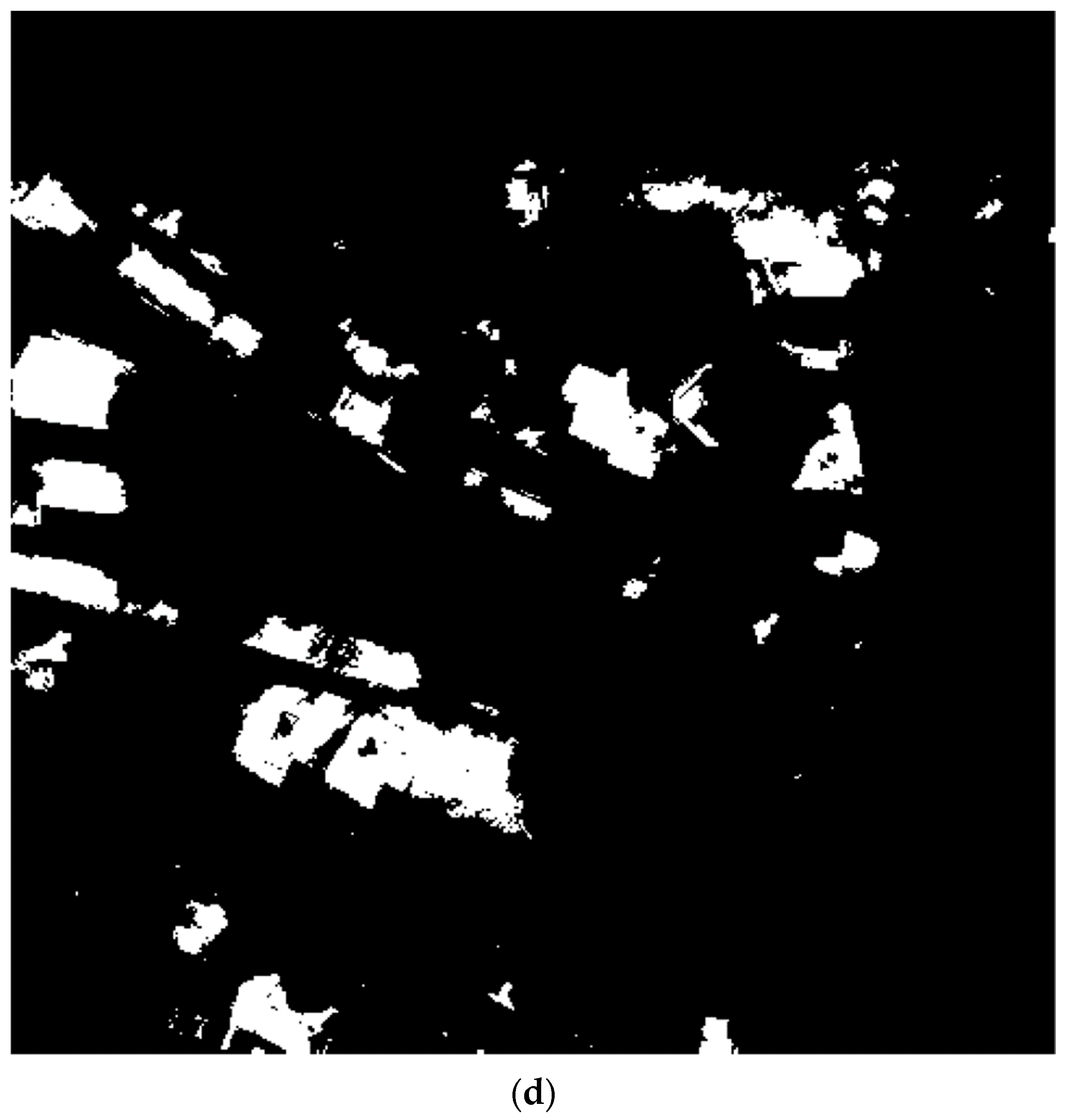
4.1.1. Assessment of Test Image A

Test image A in Figure 5a mainly consists of various vegetation cover types and shadows with irregular shapes. In this situation, the resulting images using our proposed approach, the NSVDI-based method [18] and the SDI-based method [19], as shown in Figure 5e,g,h, respectively, demonstrate a similar visual appearance to the reference image in Figure 5b. When compared with the reference image in Figure 5b, the resulting image by the SRI-based method [11] in Figure 5c shows a good result. However, this resulting image still has some shortcomings: the shapes of many shadow areas are distorted to some extent because the shape information is only preserved by the intensity component rather than both the chromaticity and the intensity. Also, some small shadow regions are more or less omitted. In addition, the resulting image obtained using the NSVDI-based method [18] shown in Figure 5d demonstrates relatively good performance. Due to the utilization of invariant color properties of saturation and intensity, this NSVDI-based method accurately highlights most shadow regions and classifies shadows against vegetation for test image A, which has high vegetation coverage. The shadow omission problem still remains because some small shadow regions are omitted in the resulting image. Furthermore, the resulting image obtained with the MC3-based method [20] shown in Figure 5e appropriately distinguishes shadow pixels from vegetation pixels. However, this method fails to detect small shadows effectively, and misclassifies some bluish vegetation pixels as shadows, because bluish pixels are highlighted in the MC3 index. Similarly, the resulting image using the SI-based method [14] shown in Figure 5f generally delineates contours of large shadow regions. Nevertheless, the small shadow omission problem is still serious: most small shadows are confused with vegetation, because vegetation pixels may present similar reflectivity as shadows in the combination of near infrared, red and blue bands. Similar to the appearance in the resulting image using the NSVDI-based method [18] shown in Figure 5d, the resulting image by the SDI-based method [19] shown in Figure 5g presents a relatively accurate shadow detection result even though vegetation pixels are misclassified as shadow pixels to some extent in comparison with the reference image in Figure 5b. As for the resulting image using our proposed MPSI-based approach in Figure 5h, most small shadow regions are correctly identified, and most vegetation pixels are correctly classified. Due to the combined contribution of both invariant color components (hue and intensity), and the near infrared band and the red band, this resulting image shows a closer appearance to the reference image in Figure 5b compared with the other comparative methods mentioned above.

4.1.2. Assessment of Test Image B

The majority of test image B in Figure 6a is vegetation, various shadow regions, and a small fraction of buildings. The resulting images by the SDI-based method [18] shown in Figure 6g and our proposed method in Figure 6h have a similar appearance to the reference image shown in Figure 6b. When compared with the reference image shown in Figure 6b separately, the resulting image using the SRI-based method [11] shown in Figure 6c accurately detects general contours of large shadow regions, and correctly identifies true shadows. However, the vegetation misclassification problem still exists, because several vegetation pixels around the boundary between shadow and vegetation are misclassified as shadows. Additionally, the NSVDI-based method [18] shown in Figure 6d performs poorly. Though shadow regions are well distinguished from buildings and red roofs, most vegetation pixels are wrongly classified as shadow pixels because vegetation pixels usually show lower saturation values than those of buildings as shown in Figure 6a. Additionally, the resulting image obtained using the MC3-based method [20] shown in Figure 6e generally delineates outlines of large shadow areas. Nevertheless, many small shadow regions are identified as nonshadow regions, many buildings are wrongly recognized as shadows, and a portion of vegetation pixels are determined as shadow pixels because this method highlights bluish pixels. Similarly, the resulting image obtained using the SI-based method [14] shown in Figure 6f performs relatively poorly compared with the reference image in Figure 6b. Though many large shadow regions were identified using this method, many small shadow regions are classified as nonshadow regions. Also, several buildings were wrongly classified as shadow regions, except that red roofs were generally separated from shadows. Furthermore, the resulting image produced by the SDI-based method [19] shown in Figure 6g demonstrates a relatively good result. Most shadow regions were correctly determined and a majority of vegetation areas were well distinguished from shadow regions. However, there are still a few number of vegetation pixels as well as buildings that are misclassified as shadows. When it comes to our proposed MPSI-based approach, the resulting image shown in Figure 6h is much closer to the reference image in Figure 6b among the examined shadow detection methods. Both large and small shadow regions are almost all correctly determined, and nonshadow regions, especially vegetation areas, are well distinguished from shadow regions. Therefore, the problems of shadow omission and vegetation misclassification are further resolved in the resulting image using our proposed approach, as shown in Figure 6h.

4.1.3. Assessment of Test Image C

To further validate the effectiveness of our proposed shadow detection approach, we compared the performance of our developed method to other investigated shadow detection methods with test image C. The test image C, as shown in Figure 7a, includes diverse land cover types (vegetation regions both in large area and individually, roads, lawns, bare soil, buildings in various profiles, etc.) and shadow regions with various irregular shapes. Under this complex scene, the resulting images produced by the SDI-based method [19] shown in Figure 7g and our proposed shadow detection approach, shown in Figure 7h, achieved the closest appearances to the reference image, as shown in Figure 7b, compared to other shadow detection methods previously mentioned as shown in Figure 7c–h. When the resulting images were individually compared with the reference image in Figure 7b, the resulting image produced by the SRI-based method [11] shown in Figure 7c generally differentiated shadow regions from roads, lawns, bare soil, and most buildings. However, a vast majority of the vegetation was wrongly classified as shadow regions as this method is sensitive to bluish or greenish properties which are often presented by vegetation pixels. Similar to Figure 6d, the resulting image produced by the NSVDI-based method [18] shown in Figure 7d generally identified shadow regions from most roads and buildings, whereas substantially all of the vegetation pixels were still misclassified as shadows because of the lower saturation values of these objects in this complex scene. Also, dark terrace roofs, lawns and bare soil were misclassified as shadows. Furthermore, the misclassification of lawns and bare soil as shadows were overcome to some extent in the resulting image produced by the MC3-based method [18], shown in Figure 7e. Though most shadow regions were reasonably outlined, many small true shadow regions actually shown in Figure 7a were omitted in the resulting image shown in Figure 7e. Additionally, this technique failed to correctly recognize shadow pixels against roads and parts of buildings, and did not accurately preserve contours of shadow regions. Similarly, the resulting image produced by the SI-based method [14], shown in Figure 7f, generally delineated the outlines of most large shadow regions. However, this method still omitted most small shadow regions and failed to preserve the shapes of shadow regions, because pixel values on the boundary between shadow and nonshadow regions cannot be accurately highlighted with this method. Additionally, the resulting image produced by the SDI-based method [19], shown in Figure 7g, presented quite good performance in terms of shadow detection. Shadow regions were correctly identified in diverse scenes, mainly including a majority of vegetation regions, roads, lawns, and bare soil. Besides, contours of shadow regions were also well persevered. Nevertheless, the small shadow omission problem remains an issue to explore. In terms of our proposed approach, the resulting image shown in Figure 7h is closer in appearance to the reference image shown in Figure 7b compared with the other investigated comparable shadow detection methods. Even though a small amount of small shadow regions within vegetation regions was omitted, our approach performed well in correctly detecting shadow regions in various shapes. Also, shadow regions were well separated apart from most nonshadow regions, especially for vegetation. Therefore, our proposed approach is an improvement in terms of the problems posed by both shadow region omission and vegetation misclassification, compared with other investigated comparable shadow detection techniques.

4.1.4. Analogy of Our Proposal among Test Images A, B, and C

To evaluate the shadow detection performance of our proposed MPSI-based approach in different scenes, we compared the appearances of resulting images shown in Figure 5h, Figure 6h and Figure 7h with corresponding reference images shown in Figure 5b, Figure 6b and Figure 7b. In these resulting images, shadow pixels were well distinguished from vegetation pixels whether the test image included a simple scene of almost all vegetation (test image A shown in Figure 5a) or a complex scene of diverse land cover types (test image B shown in Figure 6a and C shown in Figure 7a). Also, outlines of shadow regions were well delineated, even though a small amount of shadow pixels were still omitted. Comparing the appearances of the resulting images of test images A, B, and C with our proposed method shown in Figure 5h, Figure 6h and Figure 7h, respectively, we validated that the shadow regions were better recognized for test image C than in A and B. Also, the resulting image shown in Figure 7h for test image C highlights that our proposed approach works well for images with complex scenes including diverse land cover types. When comparing the performances of our shadow detection approach for test image A and B, we found that vegetation pixels and small shadow regions were well detected in both the test images, even though some dark buildings in test image B were misclassified as shadows to some extent due to their similarity to shadows. Accordingly, based on the subjective assessment, we conclude that our proposed MPSI-based shadow detection approach shows an improved ability in terms of mitigating the shadow omission and vegetation misclassification problems compared with other comparable standard shadow detection methods investigated in this paper.

4.2. Objective Assessment

In addition to the subjective assessment performed above, in this part we perform objective assessments of the images produced by comparable algorithms [11,14,18,19,20] and our proposed approach, as shown in Figure 5c–h, Figure 6c–h and Figure 7c–h. These objective assessments were carried out with metrics calculated with the confusion matrix previously reported [19,38,42,43]. The confusion matrix was achieved by comparing the reference image and the final resulting shadow image of each test image for every shadow detection approach pixel by pixel. Based on the confusion matrix, we exploited several metrics [11,13,21] for objectively evaluating accuracies of the final resulting shadow images obtained with the different detecting methods. The corresponding metrics, namely the producer’s accuracy (PA), also called sensitivity, the omitted error (EO), the specificity (SP), the committed error (EC) and the overall accuracy (OA), were calculated pixel by pixel as follows:

$$PA=\frac{TP}{\left(TP+FN\right)}$$

(22)

$$EO=\frac{FN}{\left(TP+FN\right)}$$

(23)

$$SP=\frac{TN}{\left(TN+FP\right)}$$

(24)

$$EC=\frac{FP}{\left(TN+FP\right)}$$

(25)

$$OA=\frac{TP+TN}{\left(TP+TN+FP+FN\right)}$$

(26)

where $TP$ (true positive) indicates the number of true shadow pixels correctly identified, $TN$ (true negative) is the number of nonshadow pixels correctly classified, $FP$ (false positive) refers to the number of true nonshadow pixels wrongly classified as shadows, $FN$ (false negative) shows the amount of true shadow pixels wrongly defined as nonshadows, and the terms TP + FN and TN + FP denote the amounts of shadow pixels and nonshadow pixels, respectively, and the term TP + TN + FP + FN is the total number of pixels in the study image.

Specifically, the PA indicates how well shadow pixels are correctly detected among true shadow pixels in the reference image, which is the ratio of the number of shadow pixels correctly detected in the resulting image to the total amount of the shadow pixels in the reference image. Complementarily, the EO is caused by identifying true shadow pixels in the original image as nonshadow pixels, which is the ratio of the number of nonshadow pixels in the resulting image wrongly classified from true shadow pixels to the total amount of the true shadow pixels. The higher the PA, the more accurate the method is for shadow detection. At the same time, a lower EO is also achieved, which means much fewer true shadow pixels are omitted as nonshadow pixels. A good shadow detection approach usually has a high PA value and a low EO value. Similarly, the SP denotes how well nonshadow pixels are correctly classified among true nonshadow pixels in the study image, which is the ratio of the number of nonshadow pixels correctly classified in the resulting image to the total amount of the true nonshadow pixels. Correspondingly, the EC is caused by classifying true nonshadow pixels in the original image as shadow pixels, which is presented as the ratio of the number of shadow pixels wrongly classified in the resulting image from true nonshadow pixels in the original image to the total amount of the true nonshadow pixels. The higher the SP, the better the algorithm performs for detecting shadow regions. Meanwhile, a lower EC is also obtained, which reveals that much fewer true nonshadow pixels are classified as shadow pixels. Many shadow detection approaches that are suitable for well differentiating nonshadows (e.g., vegetation regions) from shadows, usually have a high SP value and a low EC value. Additionally, the OA explains the entire effectiveness of a certain shadow detection algorithm for detecting shadow pixels. A better performance of a certain shadow detection algorithm is achieved when the OA is higher. All of these metrics described above (PA, EO, SP, EC, and OA) were employed together to assess the performance of the comparable standard shadow detection algorithms and our proposed method for detecting shadow pixels and correctly differentiating shadow pixels from vegetation. These metrics above were used to objectively demonstrate the accuracy of each shadow detection method previously reported [11,14,18,19,20] and our proposed method in terms of shadow detection accuracy, which was based on the calculation between each resulting image and the corresponding reference image at the pixel level. The achieved accuracy data are summarized in Table 1 for test image A, shown in Figure 5a, Table 2 for test image B, shown in Figure 6a, and Table 3 for test image C, shown in Figure 7a. For objectively assessing the effectiveness of our proposed shadow detection approach in detail, a further explanation is provided in terms of the accuracy data.

4.2.1. Assessment of Test Image A

For test image A in Figure 5a, the resulting image accuracy data are summarized in Table 1. From Table 1, the OA values for the NSVDI-based method [18] (88.56%), the SDI-based method [19] (91.69%), and our proposal (95.33%) are higher than those of the other three standard shadow detection approaches [11,14,20]. The high OA values for these three methods mean that they perform better in detecting shadows in general than the other three methods, which is in accordance with the corresponding subjective assessment. For the PA values and the EO values, high PA values and corresponding low EO values were achieved by the NSVDI-based method [18] (PA: 94.29%, EO: 5.71%), the SDI-based method [19] (PA: 96.18%, EO: 3.82%), and our proposed approach (PA: 95.78%, EO: 4.22%). However, rather low PA values and corresponding high EO values were obtained by the SRI-based method [11] (PA: 75.40%, EO: 24.60%), the MC3-based method [20] (PA: 86.28%, EO: 13.72%), and the SI-based method [14] (PA: 62.64%, EO: 37.36%). The PA and EO values above reveal that the NSVDI-based method [18], the SDI-based method [19] and our proposed MPSI-based approach performed better in correctly classifying shadow pixels of original shadow to the same class rather than nonshadow pixels in the produced images. They avoided omitting shadow pixels as nonshadow pixels for test image A in Figure 5a when they were compared with the three other methods above [11,14,20]. As for metrics of the SP values and the EC values, we observed that high SP values and corresponding low EC values were obtained by the SRI-based method [11] (SP: 92.98%, EC: 7.02%), the SI-based method [14] (SP: 97.03%, EC: 2.97%), and our proposed approach (SP: 94.77%, EC: 5.23%); whereas, relatively low SP values and high EC values were shown by the NSVDI-based method [18] (SP: 81.52%, EC: 18.48%), the MC3-based method [20] (SP: 73.06%, EC: 26.94%), and the SDI-based method [19] (SP: 86.16%, EC: 13.84%). The SP and EC values above show that the former three methods—the SRI-based method [11], the SI-based method [14], and our proposed approach—performed better in correctly classifying nonshadow pixels of the original images to the same class rather than as shadow pixels, and avoided wrongly identifying nonshadow pixels as shadow pixels for test image A, as shown in Figure 5a, than the three other methods. In general, even though the resulting images produced by the SRI-based method [11] and the SI-based method [14] had high SP values and corresponding low EC values, they had rather low OA values, low PA values, and corresponding high EO values. Besides, even not very high SP values and very low EC values for the two methods [18,19], they had significantly high PA values and low EO values, and high OA values. All of the above reveals the better overall performance in terms of shadow detection by the methods in Ma et al. [18] and Mostafa et al. [19] than those in Tsai [11], Chen et al. [14], and Besheer et al. [20]. When compared with the accuracy data of these shadow detection methods for test image A, as shown in Figure 5a, the PA value for our proposal (95.78%) is a little lower than that (96.18%) of the SDI-based method [19], and the SP value of our proposal (94.77%) is lower than that (97.03%) of the SI-based method [14]. Similarly, the EO value of our proposal (4.22%) is a little higher than that (3.82%) of the SDI-based method [19], and the EC value of our proposal (5.23%) is higher than that (2.97%) of the SI-based method [14]. However, the resulting accuracy data for our method are highly significant in terms of the high values of PA and SP, and the quite low values of EO and EC, as well as the highest value of OA compared to the other methods for test image A, as shown in Figure 5a, which reveals that our proposed approach performs well in both correctly identifying shadow pixels in the original images into the same class and reducing the probability of misclassifying nonshadow pixels of the original images as shadow pixels.

4.2.2. Assessment of Test Image B

For test image B in Figure 6a, the related resulting accuracy data are summarized in Table 2. From Table 2, higher values of OA are achieved in the resulting images produced by the SDI-based method [19] (93.27%) and our proposed approach (94.24%) than those by other methods [11,14,18,20], as shown in the last column of Table 2. These higher OA values mean that the SDI-based method and our method performed better generally at detecting shadow pixels than the other methods. Furthermore, for the PA values and the EO values, quite high PA values and corresponding low EO values were obtained in resulting images produced by the SRI-based method [11] (PA: 97.16%, EO: 2.84%), the NSVDI-based method [18] (PA: 99.94%, EO: 0.06%), the SDI-based method [19] (PA: 94.99%, EO: 5.01%) and our method (PA: 95.63%, EO: 4.37%). The high PA and corresponding low EO metrics of methods in Tsai [11], Ma et al. [18], and Mostafa et al. [19] and our method together reveal that shadow pixels of the original images were correctly identified, and fewer shadow pixels of the original images were omitted as nonshadow pixels for test image B in Figure 6a, when compared with other shadow detection methods in Chen et al. [14], and Besheer et al. [20]. Additionally, for the SP values and the EC values, higher SP values and corresponding lower EC values were obtained by the SI-based method [14] (SP: 93.70%, EC: 6.30%), the SDI-based method [19] (SP: 90.21%, EC: 9.79%) and our method (SP: 91.76%, EC: 8.24%) than those by other methods in Tsai [11], Ma et al. [18], and Besheer et al. [20]. These higher SP and corresponding lower EC values together show that these two standard shadow detection methods and our method are more correct when classifying nonshadow pixels in the original images to the same class rather than as shadow pixels, and lower probability of misclassifying nonshadow pixels in the original images as shadow pixels than those by other methods in Tsai [11], Ma et al. [18], and Besheer et al. [20]. Besides, even though the PA value of our method (95.63%) was a little lower than that of the SRI-based method in Tsai [11] (97.16%) and the NSVDI-based method in Ma et al. [18] (99.94%), the SP (91.76%) and OA (94.24%) values of our method were much higher than those of the above two methods. Similarly, even though the EO value of our method (4.37%) was higher than that of the SRI-based method in Tsai [11] (2.84%) and the NSVDI-based method in Ma et al. [18] (0.06%), the EC (8.24%) value of our proposal was much lower than those of the above two methods. Specifically, our method also performed better for shadow detection with a somewhat higher PA (95.63%), SP (91.76%), and OA (94.24%), as well as lower EO (4.37%), and EC (8.24%), than the SDI-based method in Mostafa et al. [19] with PA (94.99%), SP (90.21%), and OA (93.27%), as well as EO (5.01%) and EC (9.79%). Both the significant metrics of high PA and SP values, as well as low EO and EC values reveal that our method can simultaneously perform well in reducing the probability of omitting shadow pixels in the original images as nonshadows, and misclassifying nonshadow pixels in the original images as shadows for test image B, as shown in Figure 6a.

4.2.3. Assessment of Test Image C

For test image C in Figure 7a, the related accuracy data are listed in Table 3. From Table 3, higher OA values are noted in the resulting images produced by the SDI-based method in Mostafa et al. [19] (89.26%) and our proposed approach (95.50%) than those by the SRI-based method in Tsai [11] (75.60%), the NSVDI-based method in Ma et al. [18] (74.89%), the MC3-based method in Besheer et al. [20] (81.75%) and the SI-based method in Chen et al. [14] (75.06%), as shown in the last column of Table 3. These higher OA values reveal that both the SDI-based method in Mostafa et al. [19] and our approach were generally more effective at detecting shadows for test image C than other methods in Tsai [11], Chen et al. [14], Ma et al. [18], and Besheer et al. [20]. Furthermore, in terms of the PA values and the corresponding EO values, higher PA and corresponding lower EO values were obtained by the SRI-based method in Tsai [11] (PA: 98.88%, EO: 1.12%), the NSVDI-based method in Ma et al. [18] (PA: 99.72%, EO: 0.28%) and our approach (PA: 97.19%, EO: 2.81%) than those by the three other methods in Chen et al. [14], Mostafa et al. [19], and Besheer et al. [20], as shown in the second and the fourth columns of Table 3. These high PA and corresponding low EO values show the fact that shadow pixels in the original images are correctly identified, and the omission of shadow pixels in the original images is mostly avoided with these three methods (i.e., the SRI-based method in Tsai [11], the NSVDI-based method in Ma et al. [18] and our approach), when compared with those of the other shadow detection methods in Chen et al. [14], Mostafa et al. [19], and Besheer et al. [20]. Additionally, regarding the SP values and the corresponding EC values, rather high SP and low EC values were achieved by the SI-based method [14] (SP: 96.64%, EC: 3.06%), the SDI-based method [19] (SP: 94.45%, EC: 5.55%) and our method (SP: 92.10%, EC: 7.90%) in comparison with those by the other methods, the SRI-based method in Tsai [11] (SP: 28.69%, EC: 71.31%), the NSVDI-based method in Ma et al. [18] (SP: 24.87%, EC: 75.13%) and the MC3-based method in Besheer et al. [20] (SP: 76.17%, EC: 23.83%). For shadow detection methods in Chen et al. [14], Mostafa et al. [19] and our approach, the SP and corresponding EC values above reveal that nonshadow pixels in the original images were better discriminated from shadow pixels, and fewer nonshadow pixels in the original images were misclassified as shadow pixels than the other shadow detection methods in Tsai [11], Ma et al. [18] and Besheer et al. [20] for test image C in Figure 7a. Besides, the problems of shadow omission or nonshadow misclassification could be effectively resolved solely with standard shadow detection methods in Tsai [11], Chen et al. [14], Ma et al. [18], and Mostafa et al. [19], because rather high PA and low SP values, as well as low EO and high EC values, were obtained by the SRI-based method in Tsai [11] (PA: 98.88%, SP: 28.69%, EO: 1.12%, EC: 71.31%) and the NSVDI-based method in Ma et al. [18] (PA: 99.72%, SP: 24.87%, EO: 0.28%, EC: 75.13%), and quite high SP and low PA values, as well as low EC and high EO values, were obtained with the SI-based method in Chen et al. [14] (PA: 64.19%, SP: 96.64%, EO: 35.81%, EC: 3.06%) and the SDI-based method in Mostafa et al. [19] (PA: 86.68%, SP: 94.45%, EO: 13.32%, EC: 5.55%). However, our shadow detection approach was more effective at simultaneously resolving both problems of shadow omission and nonshadow misclassification than other shadow detection methods investigated in this paper, because high PA (97.19%) and SP (92.10%) values as well as low EO (2.81%) and EC (7.90%) values were achieved with our method rather than either one or none in other methods for test image C in Figure 7a.

4.2.4. Analogy of Our Proposal among Test Images A, B and C

In addition to the performance comparison of our proposed approach and other shadow detection methods in Tsai [11], Chen et al. [14], Ma et al. [18], Mostafa et al. [19] and Besheer et al. [20], we also evaluated the effectiveness of our method for detecting shadows in different scenes with accuracy data listed in the last row of Table 1, Table 2 and Table 3. As previously described, test image A is a simple scene of entirely vegetation, test image B includes mostly vegetation and a small fraction of buildings, and test image C consists of diverse land cover types including vegetation, buildings, roads, lawns, etc. Obviously, we noticed that similar OA values were achieved for test image A (95.33%), B (94.24%), and C (95.50%), which reveals that our method performed well for shadow detection in both simple vegetation scenes and complex scenes of diverse land cover. In terms of PA, SP, EO, and EC, on one hand, for the image mainly containing vegetation (i.e., test image A), higher SP (94.77%) and corresponding lower EC (5.23%) values were shown, which proves the efficacy of our method in accurately identifying vegetation pixels in the original images to the same class rather than as shadows, and reducing the probability of misclassifying vegetation pixels in the original images as shadows. Rather high PA (95.78%) and low EO (4.22%) values were shown, revealing that the problem of shadow omission was further resolved. On the other hand, for the complex image including diverse land cover types (i.e., test image C), higher PA (97.19%) and corresponding lower EO (2.81%) values were obtained, which shows that our method also performed well in correctly detecting shadow pixels in the original images as the same class rather than as nonshadows, and avoided omitting shadow pixels in original images as nonshadows as far as possible. Also, quite high SP (92.10%) and low EC (7.90%) values were achieved showing that the problem of vegetation misclassification was also further minimized. As for test image B, quite good shadow detection effectiveness was also obtained with our proposed approach.

Consequently, our developed shadow detection approach is suitable for shadow detection in both simple scenes mainly containing vegetation and complex scenes including diverse land cover types. Also, excellent performance was demonstrated for both correctly identifying shadow pixels, and discriminating shadow from nonshadow pixels, especially for vegetation cover types. In other words, our method is effective for managing both problems of shadow omission and vegetation misclassification.

5. Conclusions

In this paper, we developed and validated a new shadow detection approach based on general shadow properties including high hue and low intensity in the HSV invariant color space and special spectral reflectivity features of high reflectivity values in the near infrared band and low reflectivity values in the red band for vegetation in nonshadow regions. A rough shadow image was first produced using these properties, in which shadow pixels were highlighted and nonshadow pixels were depressed. Then, the final shadow image was drawn with a certain threshold on the rough shadow image. For the validation of our method, comparative experiments were applied over three test images selected from the multispectral WorldView-3 remote sensing image of Rio de Janeiro, Brazil. The performance of our developed mixed property-based shadow detection approach was compared with other comparable shadow detection methods [11,14,18,19,20], after which the resulting experimental data were evaluated both subjectively and objectively. The resulting experimental data revealed that images produced by our method had much closer appearances to the reference images and excellent accuracy metrics, namely high average values for the overall accuracy (95.02%), the producer’s accuracy (96.20%), and the specificity (92.87%), and low average values for the omitted error (3.80%) and the committed error (7.12%), when compared with those of other comparable shadow detection methods. Both the good visual sense and excellent accuracy metrics reveal that our approach makes an improvement for simultaneously further addressing the problems of shadow omission and vegetation misclassification. In the future, we will attempt to improve the shadow detection accuracy and decrease the computational time in a further step. Combined with our current work, we will simultaneously attempt to better distinguish shadows from water.

References

1. Murthy, K.; Shearn, M.; Smiley, B.D.; Chau, A.H.; Levine, J.; Robinson, M.D. Skysat-1: Very high-resolution imagery from a small satellite. In Proceedings of the Sensors, Systems, and Next-Generation Satellites XVII, Amsterdam, The Netherlands, 22–25 September 2014. [Google Scholar] [CrossRef]
2. Qu, H.S.; Zhang, Y.; Jin, G. Improvement of performance for CMOS area image sensors by TDI algorithm in digital domain. Opt. Precis. Eng. 2010, 18, 1896–1903. [Google Scholar] [CrossRef]
3. Lan, T.J.; Xue, X.C.; Li, J.L.; Han, C.S.; Long, K.H. A high-dynamic-range optical remote sensing imaging method for digital TDI CMOS. Appl. Sci. 2017, 7, 1089. [Google Scholar] [CrossRef]
4. Fauvel, M.; Chanussot, J.; Benedictsson, J.A. A spatial-spectral kernel-based approach for the classification of remote-sensing images. Pattern Recognit. 2012, 45, 381–392. [Google Scholar] [CrossRef]
5. Marcello, J.; Medina, A.; Eugenio, F. Evaluation of spatial and spectral effectiveness of pixel-level fusion techniques. IEEE Geosci. Remote Sens. Lett. 2013, 10, 432–436. [Google Scholar] [CrossRef]
6. Eugenio, F.; Marcello, J.; Martin, J. High-resolution maps of bathymetry and benthic habits in shallow-water environments using multispectral remote sensing imagery. IEEE Trans. Geosci. Remote Sens. 2015, 53, 3539–3549. [Google Scholar] [CrossRef]
7. Martin, J.; Eugenio, F.; Marcello, J.; Medina, A. Automatic sun glint removal of multispectral high-resolution WorldView-2 imagery for retrieving coastal shallow water parameters. Remote Sens. 2016, 8, 37. [Google Scholar] [CrossRef]
8. Marcello, J.; Eugenio, F.; Perdomo, U.; Medina, A. Assessment of atmospheric to retrieve vegetation in natural protected areas using multispectral high resolution imagery. Sensors 2016, 16, 1624. [Google Scholar] [CrossRef] [PubMed]
9. Zhao, J.; Zhong, Y.F.; Shu, H.; Zhang, L.P. High-resolution image classification integrating spectral-spatial-location cues by conditional random fields. IEEE Trans. Image Process. 2016, 25, 4033–4045. [Google Scholar] [CrossRef] [PubMed]
10. Huang, S.Y.; Miao, Y.X.; Yuan, F.; Gnyp, M.L.; Yao, Y.K.; Cao, Q.; Wang, H.Y.; Lenz_Wiedemann, V.I.; Bareth, G. Potential of RapidEye and WorldView-2 satellite data for improving rice nitrogen status monitoring at different growth stages. Remote Sens. 2017, 9, 227. [Google Scholar] [CrossRef]
11. Tsai, V.J. A comparative study on shadow compensation of color aerial images in invariant color models. IEEE Trans. Geosci. Remote Sens. 2006, 44, 1661–1671. [Google Scholar] [CrossRef]
12. Khekade, A.; Bhoyar, K. Shadow detection based on RGB and YIQ color models in color aerial images. In Proceedings of the 1st International Conference on Futuristic Trend in Computational Analysis and Knowledge Management (ABLAZE 2015), Greater Noida, India, 25–27 February 2015. [Google Scholar]
13. Liu, J.H.; Fang, T.; Li, D.R. Shadow detection in remotely sensed images based on self-adaptive feature selection. IEEE Trans. Geosci. Remote Sens. 2011, 49, 5092–5103. [Google Scholar] [CrossRef]
14. Chen, H.S.; He, H.; Xiao, H.Y.; Huang, J. Shadow detection in high spatial resolution remote sensing images based on spectral features. Opt. Precis. Eng. 2015, 23, 484–490. [Google Scholar] [CrossRef]
15. Kim, D.S.; Arsalan, M.; Park, K.R. Convolutional neural network-based shadow detection in images using visible light camera sensor. Sensors 2018, 18, 960. [Google Scholar] [CrossRef] [PubMed]
16. Schläpfer, D.; Hueni, A.; Richter, R. Cast shadow detection to quantify the aerosol optical thickness for atmospheric correction of high spatial resolution optical imagery. Remote Sens. 2018, 10, 200. [Google Scholar] [CrossRef]
17. Wu, J.; Bauer, M.E. Evaluating the effects of shadow detection on QuickBird image classification and spectroradiometric restoration. Remote Sens. 2013, 5, 4450–4469. [Google Scholar] [CrossRef]
18. Ma, H.J.; Qin, Q.M.; Shen, X.Y. Shadow segmentation and compensation in high resolution satellite images. In Proceedings of the IEEE International Geoscience and Remote Sensing Symposium (IGARSS 2008), Boston, MA, USA, 7–11 July 2008. [Google Scholar]
19. Mostafa, Y.; Abdelhafiz, A. Accurate shadow detection from high-resolution satellite images. IEEE Geosci. Remote Sens. Lett. 2017, 14, 494–498. [Google Scholar] [CrossRef]
20. Besheer, M.; Abdelhafiz, A. Modified invariant color model for shadow detection. Int. J. Remote Sens. 2015, 36, 6214–6223. [Google Scholar] [CrossRef]
21. Arevalo, V.; Gonzalez, J.; Ambrosio, G. Shadow detection in color high-resolution satellite images. Int. J. Remote Sens. 2008, 29, 1945–1963. [Google Scholar] [CrossRef]
22. Kang, X.D.; Huang, Y.F.; Li, S.T.; Lin, H.; Benediktsson, J.A. Extended random walker for shadow detection in very high resolution remote sensing images. IEEE Trans. Geosci. Remote Sens. 2018, 55, 867–876. [Google Scholar] [CrossRef]
23. Wang, Q.J.; Yan, L.; Yuan, Q.Q.; Ma, Z.L. An automatic shadow detection method for VHR remote sensing orthoimagery. Remote Sens. 2017, 9, 469. [Google Scholar] [CrossRef]
24. Li, J.Y.; Hu, Q.W.; Ai, M.Y. Joint model and observation cues for single-image shadow detection. Remote Sens. 2016, 8, 484. [Google Scholar] [CrossRef]
25. Salvador, E.; Cavallaro, A.; Ebrahimi, T. Cast shadow segmentation using invariant color features. Comput. Vis. Image Understand. 2004, 95, 238–259. [Google Scholar] [CrossRef] [Green Version]
26. Huang, J.J.; Xie, W.X.; Tang, L. Detection of and compensation for shadows in colored urban aerial images. In Proceedings of the 5th World Congress on Intelligent Control and Automation, Hangzhou, China, 15–19 June 2004. [Google Scholar]
27. Song, H.H.; Huang, B.; Zhang, K.H. Shadow detection and reconstruction in high-resolution satellite images via morphological filtering and example-based learning. IEEE Trans. Geosci. Remote Sens. 2014, 52, 2545–2554. [Google Scholar] [CrossRef]
28. Zhang, H.Y.; Sun, K.M.; Li, W.Z. Object-oriented shadow detection and removal from urban high-resolution remote sensing images. IEEE Trans. Geosci. Remote Sens. 2014, 52, 6972–6982. [Google Scholar] [CrossRef]
29. Chung, K.L.; Lin, Y.R.; Huang, Y.H. Efficient shadow detection of color aerial images based on successive thresholding scheme. IEEE Trans. Geosci. Remote Sens. 2009, 47, 671–682. [Google Scholar] [CrossRef]
30. Otsu, N. A threshold selection method from gray-level histograms. IEEE Tans. Syst. Man Cybern. 1979, 9, 62–66. [Google Scholar] [CrossRef]
31. Sarabandi, P.; Yamazaki, F.; Matsuoka, M.; Kiremidjian, A. Shadow detection and radiometric restoration in satellite high resolution images. In Proceedings of the 2004 IEEE International Geoscience and Remote Sensing Symposium (IGARSS 2004), Anchorage, AK, USA, 20–24 September 2004. [Google Scholar]
32. Gevers, T.; Smeulders, A.W. Color-based object recognition. Pattern Recognit. 2001, 32, 453–464. [Google Scholar] [CrossRef]
33. Fan, J.L.; Lei, B. A modified valley-emphasis method for automatic thresholding. Pattern Recognit. Lett. 2012, 33, 703–708. [Google Scholar] [CrossRef]
34. Gonzalez, R.C.; Woods, R.E. Digital Image Processing, 3rd ed.; Publishing House of Electronics Industry: Beijing, China, 2010; pp. 58–65. ISBN 978-7-121-10207-3. [Google Scholar]
35. Phong, B.T. Illumination for computer generated pictures. Commun. ACM 1975, 18, 311–317. [Google Scholar] [CrossRef] [Green Version]
36. Shafer, S.A. Using color to separate reflection component. Color Res. Appl. 2010, 10, 210–218. [Google Scholar] [CrossRef]
37. Gevers, T.; Smeulders, A.W. PicToSeek: Combining color and shape invariant features for image retrieval. IEEE Trans. Image Process. 2000, 9, 102–119. [Google Scholar] [CrossRef] [PubMed]
38. Sun, J.B. Principles and Applications of Remote Sensing, 3rd ed.; Wuhan University Press: Wuhan, China, 2013; pp. 18–21, 220–222. ISBN 978-7-307-10761-8. [Google Scholar]
39. Janesick, B.J. Dueling Detectors. SPIE Newsroom 2002, 30–33. [Google Scholar] [CrossRef]
40. DG2017_WorldView-3_DS. Available online: https://dg-cms-uploads-production.s3.amazonaws.com/up-loads/document/file/95/DG2017_WorldView-3_DS.pdf (accessed on 25 July 2018).
41. Ng, H.F. Automatic thresholding for defect detection. In Proceedings of the Third International Conference on Image and Graphics (ICIG’04), Hong Kong, China, 18–20 December 2004. [Google Scholar]
42. Story, M.; Congalton, R.G. Accuracy assessment: A user’s perspective. Photogramm. Eng. Remote Sens. 1986, 52, 397–399. [Google Scholar]
43. Congalton, R.G.; Green, K. Assessing the Accuracy of Remotely Sensed Data: Principles and Practices, 2nd ed.; CRC Press: Boca Raton, FL, USA, 1999; pp. 56–61. ISBN 0-87371-986-7. [Google Scholar]
Figure 1. Sampling curves regarding the difference values between the hue component and the intensity component in both shadow and nonshadow regions.
Applsci 08 01883 g001
Figure 2. Sampling curves with respect to the reflectivity difference values between the normalized reflectivity values of the red (R) band and the near infrared (NIR) band for both shadow regions and vegetation cover types in nonshadow regions.
Applsci 08 01883 g002
Figure 3. Flow chart of the proposed mixed property-based shadow detection approach.
Applsci 08 01883 g003
Figure 4. Test images. (a) The multispectral WorldView-3 remote sensing image of Rio de Janeiro, Brazil. (b) The test image A. (c) The test image B. (d) The test image C.
Applsci 08 01883 g004
Figure 5. Test image A. (a) The original image. (b) The reference shadow image. (c) Shadow image by the spectral ratio index (SRI)-based algorithm [11]. (d) Shadow image by the normalized saturation value difference index (NSVDI)-based algorithm [18]. (e) Shadow image by the modified C3 (MC3)-based algorithm [20]. (f) Shadow image by the shadow intensity (SI)-based algorithm [14]. (g) Shadow image by the shadow detector index (SDI)-based algorithm [19]. (h) Shadow image by the developed mixed property-based shadow index (MPSI)-based approach.
Applsci 08 01883 g005aApplsci 08 01883 g005bApplsci 08 01883 g005cApplsci 08 01883 g005dApplsci 08 01883 g005eApplsci 08 01883 g005fApplsci 08 01883 g005gApplsci 08 01883 g005h
Figure 6. Test image B. (a) The original image. (b) The reference shadow image. (c) Shadow image by the SRI-based algorithm [11]. (d) Shadow image by the NSVDI-based algorithm [18]. (e) Shadow image by the MC3-based algorithm [20]. (f) Shadow image by the SI-based algorithm [14]. (g) Shadow image by the SDI-based algorithm [19]. (h) Shadow image by the developed MPSI-based approach.
Applsci 08 01883 g006aApplsci 08 01883 g006bApplsci 08 01883 g006cApplsci 08 01883 g006dApplsci 08 01883 g006eApplsci 08 01883 g006fApplsci 08 01883 g006gApplsci 08 01883 g006h
Figure 7. Test image C. (a) The original image. (b) The reference shadow image. (c) Shadow image by the SRI-based algorithm [11]. (d) Shadow image by the NSVDI-based algorithm [18]. (e) Shadow image by the MC3-based algorithm [20]. (f) Shadow image by the SI-based algorithm [14]. (g) Shadow image by the SDI-based algorithm [19]. (h) Shadow image by the developed MPSI-based approach.
Applsci 08 01883 g007aApplsci 08 01883 g007bApplsci 08 01883 g007cApplsci 08 01883 g007dApplsci 08 01883 g007eApplsci 08 01883 g007fApplsci 08 01883 g007gApplsci 08 01883 g007h