Enhancement of Ultrasonic Guided Wave Signals Using a Split-Spectrum Processing Method

1
TWI Ltd., Granta Park, Great Abington, Cambridge CB21 6AL, UK
2
Brunel University London, Institute of Materials and Manufacturing, Kingston Lane, Uxbridge UB8 3PH, UK
*
Author to whom correspondence should be addressed.
Appl. Sci. 2018, 8(10), 1815; https://doi.org/10.3390/app8101815
Submission received: 10 August 2018
/
Revised: 24 September 2018
/
Accepted: 29 September 2018
/
Published: 3 October 2018
(This article belongs to the Special Issue Ultrasonic Guided Waves)
Abstract
:Ultrasonic guided wave (UGW) systems are broadly utilised in several industry sectors where the structural integrity is of concern, in particular, for pipeline inspection. In most cases, the received signal is very noisy due to the presence of unwanted wave modes, which are mainly dispersive. Hence, signal interpretation in this environment is often a challenging task, as it degrades the spatial resolution and gives a poor signal-to-noise ratio (SNR). The multi-modal and dispersive nature of such signals hampers the ability to detect defects in a given structure. Therefore, identifying a small defect within the noise level is a challenging task. In this work, an advanced signal processing technique called split-spectrum processing (SSP) is used firstly to address this issue by reducing/removing the effect of dispersive wave modes, and secondly to find the limitation of this technique. The method compared analytically and experimentally with the conventional approaches, and showed that the proposed method substantially improves SNR by an average of 30 dB. The limitations of SSP in terms of sensitivity to small defects and distances are also investigated, and a threshold has been defined which was comparable for both synthesised and experimental data. The conclusions reached in this work paves the way to enhance the reliability of UGW inspection.
1. Introduction
Long-range ultrasonic testing (LRUT), also known as guided wave testing (GWT) is an advanced non-destructive testing (NDT) method that utilises ultrasonic guided wave (UGW) signals for the inspection. This inspection could be applied to any large complex structures such as pipes, rails, cables, etc. for defect detection. This method is widely utilised for the inspection of pipelines that mainly contain oil and gas products, and it has the ability to screen long distances (up to 50 m in each direction) from a single location to identify defects in the structure (e.g., corrosion, erosion) [1,2,3]. GWT often operates at a low-frequency range (20–100 kHz) (compared to conventional ultrasonic testing (UT), which operates at MHz range) to transmit the waves using one or more rings of dry-coupled transducers around the circumference of the pipe, which are pneumatically forced against the surface. These waves propagate within the pipe wall along the pipe’s main axis, and scattering occurs when the waves encounter discontinuities in wall thickness. The transducers are used to record these changes to obtain information about the presence and characteristics of the features within a pipe [4].
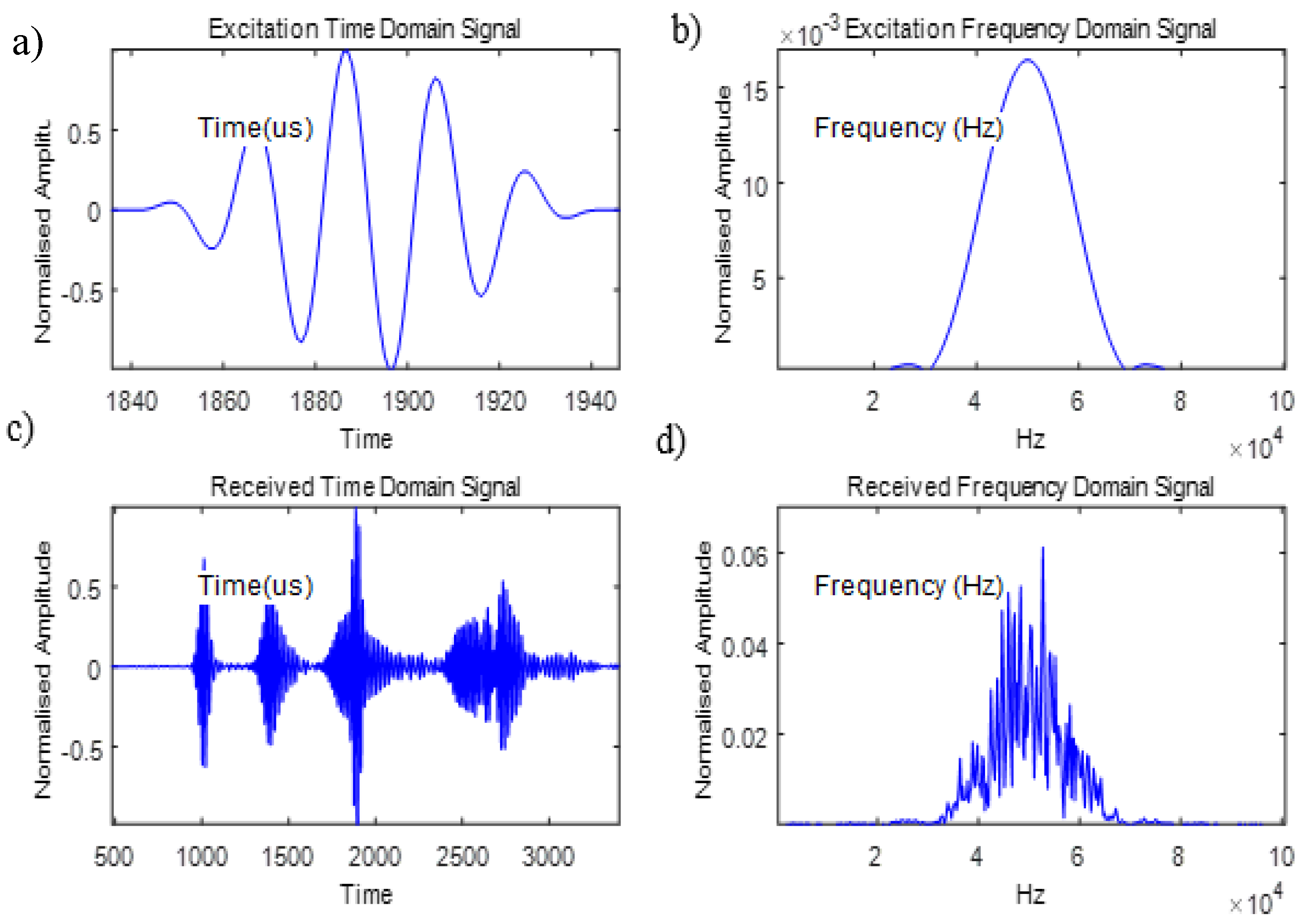
In order to reduce the effect of dispersion and to achieve a good resolution between features, a tone burst signal is employed for the transmission of the signal, as shown in Figure 1a.
This is a 50 kHz 5-cycle Hann windowed excitation signal, with a frequency response as shown in Figure 1b, which are generated in this work using MatLab software. A typical response is illustrated in Figure 1c, which consists of a number of peaks that correspond to reflections from structural features under investigation (e.g., defects and welds). In addition, its frequency response is displayed in Figure 1d, exhibiting the same frequency bandwidth as the input signal [5].
It is ideal to generate an axisymmetric wave mode to promote non-dispersive propagation; however, the interaction of the guided wave signal with non-axisymmetric features within the pipeline can cause mode conversion. This results in the generation of dispersive wave modes (DWM) that travel with different velocities according to the different frequency components in the signal [6]. Hence, the energy spreads over space during propagation, and compromises the ability to distinguish echoes from closely spaced reflectors. This lack of spatial resolution leads to coherent noise and reduces the sensitivity of the inspection. In order to enhance the sensitivity and the SNR of such signals, it is vital to minimise the presence of coherent noise. Dispersion is one of the main sources of coherent noise; hence, the aim of this work is to reduce the effect of dispersive wave modes.
There are many researchers who study the effect of dispersion in GWT [7,8,9,10,11,12,13,14]. Wilcox [7] developed a method for reversing the effect of dispersion by using the knowledge of wave mode characteristics to map signals from the time to the distance domain, and then reversed the effect of DWM and restored them to undispersed pulses. Zeng and Lin [8] investigated the dispersion pre-compensation method using chirp-based narrowband excitation signals to compress the time duration of received wave packets during the extracting process. They employed the benefits of chirp excitation by utilising previous knowledge of the dispersion curve and the propagation distance. Other researchers such as Xu et al. [9,10,11] employed dispersion compensation (DC) to analyse the propagation behaviours of the signals. However, most of them required the knowledge of the propagation distance in advance. Toiyama and Hayashi [12] combined the DC method with a pulse compression (PuC) algorithm by employing a chirp signal. They considered a scenario of a single wave mode without introducing the quantitative SNR enhancement. The combination of DC with PuC is utilised by Yucel et al. [13,14] to enhance the SNR of UGW response employing a broadband maximal length sequence excitation signal. The result showed that the technique was successful for highly dispersive flexural wave modes, but it was not that effective for longitudinal wave modes that are not dispersive. Mallet et al. [5] considered cross-correlation and wavelet de-noising algorithms for reduction of the effect of dispersion in UGW. He claimed that neither of these methods was suitable for the reduction of coherent noise, as both methods removed the smaller amplitudes regardless of whether or not they were signal or noise.
Newhouse et al. [15] considered split-spectrum processing (SSP) in the field of NDT to enhance the SNR by splitting the signal’s response into a set of sub-band signals. A theoretical basis for the selection of filter bank parameters was investigated by Karpur et al. [16]. They proposed an equation to predict SNR enhancement by compounding a number of frequency diverse signals. The result showed that some parameters achieved a larger value than expected, which could be the result of using the Gaussian function for filtering (because of its simplicity) while the calculation was based on the Sinc function. Shankar et al. [17] employed a polarity thresholding (PT) algorithm for the detection of a single target. They showed how sensitive the SNR enhancement was to the selection of filter bank parameters. Saniie et al. [18] investigated the performance of order statistic (OS) filters in conjunction with SSP in the context of ultrasonic flaw detection, to improve the flaw-to-clutter ratio of backscattered signals. It has been claimed that the OS filter performs well where the flaw and clutter echoes have good statistical separation in a given quartile. However, its performance deteriorated with the contamination from unwanted statistical information.
Gustafsson and Stepinski [19] adapted an SSP method using an artificial neural network (ANN) to implement PT for UT signals. In order to allow the relative importance of the different sub-bands to be taken into account, weighting factors were added to the input signal. The results showed better performance than, PT but only for one particular sample. Gustafsson [20] then extended the method by employing both the filter bank and the non-linear processing as an ANN for SSP. This method was time-consuming, although the results indicated that the ANN could “eliminate most of the noise”. Rubbers and Pritchard [21] developed a complex-plane SSP (CSSP) method, which was a modified version of SSP for the ultrasonic inspection of castings, and improved the SNR for a number of conventional UT techniques. It utilised an additional mathematical dimension to improve the result, while maintaining linearity in both the amplitude and the energy content of a defect signal. Moreover, they gave an overview of SSP methods [22] with a variety of SSP reconstruction algorithms and parameters. However, they claimed that as the amplitude of the processed signal is non-linear, it does not allow for the sizing of flaws, hence the use of this method is limited.
Rodriguez et al. [23,24] proposed a new filter bank design for SSP, based on the use of variable bandwidth filters, where filters were equally spaced in frequency and their energy gain equalised. They utilised stationary models for the grain noise in the presence of a single defect. They claimed that a frequency multiplication (FM) algorithm gave the greatest SNR enhancement. They stated that the number of filter bands compared to other algorithms is reduced; hence, it reduced the system complexity. However, this technique was not evaluated for non-stationary models, highly dispersive material, or a model with multiple defects. Syam and Sadanandan [25] employed a combination of SSP and order statistic filters to reduce the effect of reverberation for flaw detection in conventional UT using a wideband signal. He stated that by processing the multiple echoes corresponding to a set of transmitted signals, the effect of microstructure reflections could be suppressed with respect to the flaw echo. However, this method tested for a simulated signal only, without revealing the value of the SSP parameters.
Overall, it is clearly shown by some of the cited literature [7,8,9,10,11,12,13,14] that their techniques required prior knowledge of the dispersion curve and/or propagation distance in order to perform well. Other cited literature [15,16,17,18,19,20,21,22,23,24,25] indicated that the successful implementation of the SSP technique was highly sensitive to the selection of filter bank parameters. Although most of these papers claimed that they enhanced the SNR of the signal’s response, the enhancement was mainly achieved for conventional UT. However, those parametric values are not suitable for use in GWT that contain a combination of axisymmetric and non-axisymmetric wave modes with different phase velocities. Hence, a full study is required to find the optimum filter bank parameters for SSP in terms of its capacity to provide such improvements in GWT. To the best of the authors’ knowledge, prior to this study, apart from Mallet et al. [5], no one else has investigated the use of SSP in guided wave testing.
An analysis of SSP with application to GWT was conducted in our previous paper [26] for reducing the effects of DWMs in the signal response, and the optimum parameters have been proposed to enhance the SNR and spatial resolution of such signals. However, the limitations of SSP for use in GWT are still unclear, and they need further investigation. Hence, in this paper, the optimum parameters that were identified in the previous work are utilised for deeper investigation to improve the SNR, and to enhance the spatial resolution further by investigating the limitations of SSP mainly in two areas: (i) in terms of defect sensitivity and (ii) in terms of minimum distance between two features (e.g., weld and defect). Thus, the core concept explored in this work is to address these issues. Such a parametric study has not been undertaken in the field of GWT prior to this work.
In order to do this, a synthesised signal has been created to identify the limitations of SSP. The limitations have been tested, evaluated, and identified synthetically in a controlled environment. Then, in order to validate the effectiveness of the technique, laboratory experiments have been carried out on an eight-inch pipe utilising the Teletest-guided wave system [27]. It is shown that the proposed method reduces the presence of coherent noise and improves the SNR by up to 30 dB. In addition, the limitations of SSP have been identified and a threshold has been defined, below which the temporal resolution will be reduced.
The paper is organised as follows: Section 2 describes the theory and concept of SSP, including the implementation and selection of filter bank parameters for guided wave testing. Section 3 and Section 4 provide details and discussion of SSP for synthesised and experimental testing, and finally Section 5 concludes the paper.
2. Split-Spectrum Processing (SSP)
2.1. Theory of SSP
SSP is an advanced signal processing technique that was initially developed from the frequency agility techniques used in radar [28]. This method was then considered for SNR enhancement in NDT applications such as conventional UT, to reduce grain scatter in the received signal. A significant amount of research has been undertaken over the last few decades in this area with respect to the reduction of non-random noise (coherent noise) in NDT applications, due to ultrasonic scattering. The application of SSP in GWT is relatively new and, to the best of the authors’ knowledge, this technique and its limitations have not been previously investigated in this field.
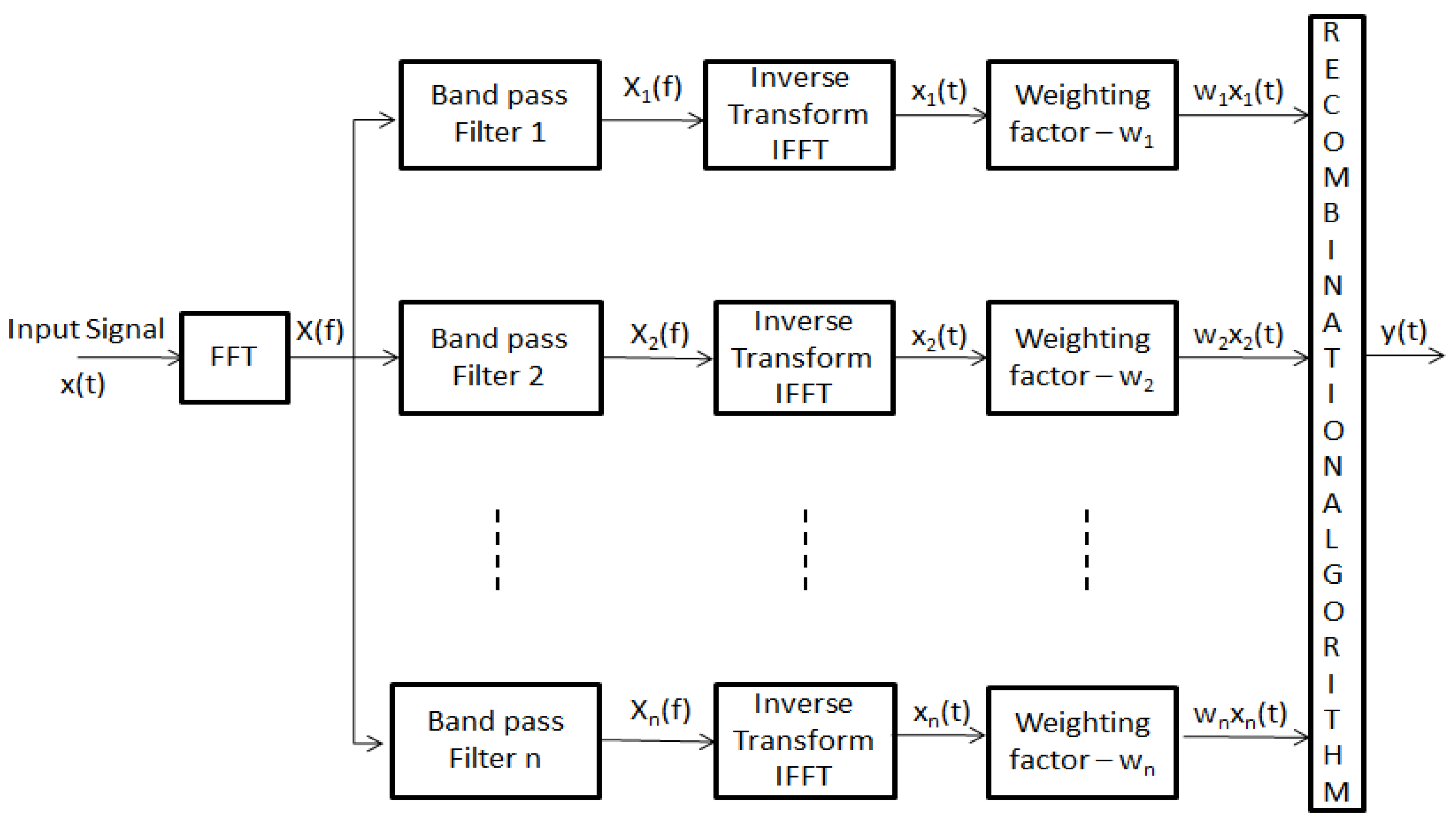
SSP splits the spectrum of a received signal in the frequency domain using a bank of bandpass filters to generate a set of sub-band signals at incremental centre frequencies. These sub-band signals are normalised and then subjected to a number of possible non-linear processing algorithms to generate an output signal. Figure 2 illustrates a block diagram for SSP with its step-by-step implementation. It shows that the input time domain signal, x(t), is transformed into the frequency domain, , using a fast Fourier Transform (FFT), and is then filtered by a bank of band-pass filters. Subsequently, the outputs from the filter banks, are converted back into the time domain using the inverse FFT (IFFT) and normalised by a weighting factor, . Then one of the recombination algorithms will be employed to combine these non-linear signals to produce the output signal . In general, SSP application shows a great potential to reduce those signal components that vary across a frequency range, in particular dispersive wave modes, and to suppress the regions of the signal of interest that are constant in that frequency range [29].
2.2. SSP Filter Bank Parameters
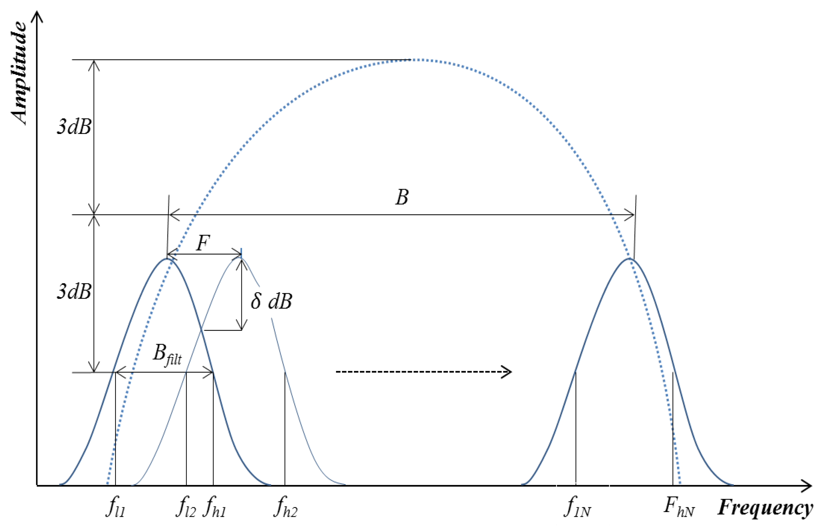
The SSP filter-bank parameters were first investigated by trial-and-error for NDT applications as they were processed. However, this was not very practical for field inspection as there are typically large amounts of data to analyse; therefore, researchers sought to find the optimum values for NDT methods. Hence, the optimum values have been proposed, developed and examined for UT techniques. However, these values are not suitable for GWT due to the long duration and narrow bandwidth of the signal that operates in the kHz range, whereas traditional UT operates in the MHz range. Therefore, further investigation was required to find an optimum value suitable for GWT. As a result, the rules and key factors of parameter selection for conventional UT have been reviewed and then modified for use in GWT. Figure 3 illustrates the scheme of SSP filtering. The parameters that need to be quantified are listed below with a brief description:
- The total bandwidth for processing (B); this needs to be large enough such that the reflections of the signal from features in the specimen are constant across this range, and the reflections from coherent noise vary. If the bandwidth is too large, then it may cause the features to be lost, as at least one of the filter outputs will not contain the feature signal. Hence it reduces the spatial resolution in the processing. In general, narrowband waveforms were used as the excitation signals to reduce the effect of unwanted wave modes, and to suppress the dispersion effect in the GWT response. Hence, the bandwidth of the transmitted signal could be employed as the total bandwidth of processing.
- The filter separation (F); is the distance between the sub-band filters. Karpur et al. [16] claimed that the optimum spectral splitting could be attained by using the frequency-sampling theorem, whereby the spectrum of a time-limited signal can be reconstructed from sample points in the frequency domain separated by 1/T Hz, where T is the total duration of the signal. Note that the Gaussian filter is employed for calculating the filter bank in practice, due to its simplicity, whereas the Sinc function was utilised for actual calculation. Thus, the filter separation could be calculated as F = 1/T.
- The sub-band filter bandwidth () is the width to be used for each filter in the filter bank. It was recommended [15,16,17] that the value of the sub-band filter bandwidth needs to be set at three to four times the filter separation. It should be noted that a bandpass filter could reduce the temporal resolution of the signal. This is because reducing the bandwidth of a time-limited signal will increase its duration. This means that the SSP filter bank needs to be selected precisely, otherwise it could lead to a reduction in temporal resolution, as the pulses that correspond to reflections from features spread out in time and mask one another. Moreover, the correlation between adjacent sub-bands could be affected by the overlap of the filters. This means the correlation increases with an increase in overlaps. On the other hand, little or no overlap could lead to loss of information. It is notable that the noise in adjacent filters needs to be uncorrelated and the features should be correlated. Hence, the overlap needs to be selected somehow to minimise the correlation between coherent noise regions in adjacent sub-bands without losing information.
- The filter crossover point (); or a cutoff frequency at the edges, is a boundary in the frequency response at which the energy flowing through the structure starts to decrease rather than passing through.
- The number of filters (); is the number of sub-band filters that is required to be selected in order to enhance the SNR and spatial resolution by correlating the signal of interest and minimising the correlation between the coherent noise region in the adjacent sub-bands signal. Overall, these parameters are dependent on each other, which means that their values have a direct effect on other parameter values. Therefore, it is necessary to search for the optimum parameters and to select them appropriately. As an example, increasing the number of filters (N) would be required to increase the total bandwidth (B), or to reduce the filter separation (F), or a combination of both. Thus, as is shown in Figure 3 the number of filters (N) could be calculated as below:
2.3. Recombination Algorithms of SSP
There are numerous SSP recombination algorithms that could be employed for use in GWT to reduce the effect of coherent noise which have been described in the literature [16,22]. In this paper, the two most common ones that obtained the highest SNR and spatial resolution in the previous work are explained in more detail:
The polarity thresholding (PT) that is expressed as:
where is the output result of the signal that is obtained after processing at m, n is the number of filter band signals, x[m] is the unprocessed signal, and [m] care the sub-band signals. This method looks at the signal sub-bands at each sample time, and if the samples are all negative or all positive, then the output is the unchanged input signal. Otherwise, the output is zero. This has the effect of only passing the time samples where the polarity is not affected by the frequency. Thus, those sections of the signal that are highly frequency-dependent must be removed. However, the amplitude of the signal of interest needs to be larger than the amplitude of the coherent noise response, whereas if the noise signal has greater amplitude, then it will change the signal’s sign.
Polarity thresholding with minimisation (PTM), which is defined as:
PTM is the combination of the minimisation and the PT algorithm where the output is the minimum amplitude of PT when there is no change in polarity. This method takes the minimum points that the PT algorithm has passed in order to suppress the noise even further than is obtained by the PT algorithm. Since the variance of the points containing noise is generally larger than those that are containing the signal of interest, the use of the minimisation algorithm reduces those that are the result of noise. However, this method is less effective when the noise level is larger than the actual signal’s amplitude; thus, reducing the noise level will significantly reduce the signal amplitude in certain sub-bands, and gives minimum values for the PTM’s output in that region.
2.4. Implementation of the Filter Bank
A MatLab program has been written that takes an unprocessed signal in the time domain and converts it to the frequency domain. It then filters the signal using a Gaussian bandpass filter to generate a set of sub-band signals, and applies the recombination algorithms into these sub-bands. The input is the signal to be filtered, with the upper and lower 3 dB cut-off frequencies. Therefore, the lower cut-off frequency , and the higher cut-off frequency , for each sub-band filter, are calculated as:
where F is the filter separation, N is the number of filters, is the lower cut-off frequency of B, and are the sub-band filters. The lower cut-off frequency for the first sub-band , needs to cover the start point of the signal. The selections of these values are inspired by the values that have been employed in UT, and then adjusted for the use in GWT using the brute force search algorithm. Table 1 shows the optimum values of SSP that were proposed in the previous paper [26]. These values are employed in this paper to find the limitations of SSP. The performance of the proposed technique is quantified by measuring the SNR, the spatial resolution, and the defect sensitivity of the output signal.
3. Signal Analysis
This section shows how this methodology has been evaluated. Initially, signals have been simulated using the technique that was presented by Wilcox [7] to represent the guided wave reflections in a pipe with known dispersion characteristics. This allows the SSP limitation to be found under controlled conditions. Secondly, experimental data was collected from an eight inch pipe that was equivalent to the simulated pipe. This gives two benefits: (i) it allows the approach to be tested under more realistic conditions; and (ii) the reusable SSP parameters across equivalent pipes could be evaluated.
Signal Synthesis
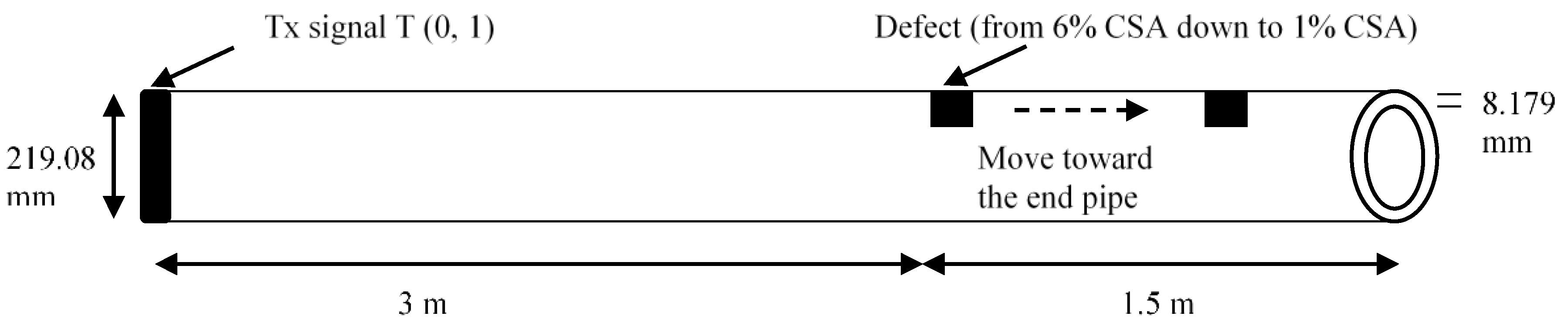
The signal synthesis was utilised to generate the propagation of the dispersive wave modes in time/space, based on applying a frequency-dependent phase shift to the wave packet of interest via DISPERSE software (developed by Imperial College, London, UK) [30]. The core concept of this section was to identify the limitation of SSP in terms of finding the smallest defect size that could be detected, and to find the distance limitation when the location of the defect is close to a dominant feature with a high amplitude, such as a weld. In order to achieve that, the axisymmetric T(0,1) wave mode is excited with a 10-cycle pulse and a centre frequency of 44 kHz, using the synthesised model. It is assumed that there are only two reflection echoes (i) from the defect, and (ii) from the pipe’s end. Since the proposed method has already proved its capability to remove the DWM [26], here, it is assumed that only the T(0,1) wave mode is reflected from the features on the pipe. According to Böttger et al. [31], there is a linear relationship between the amplitude of the reflected signal of T(0,1) and the cross-section area (CSA) of its defect. Hence, the attenuation of T(0,1) is linear, which means that if 10% of the excited signal reflects from the defect, then the rest of the energy (90%) will reflect from the pipe end.
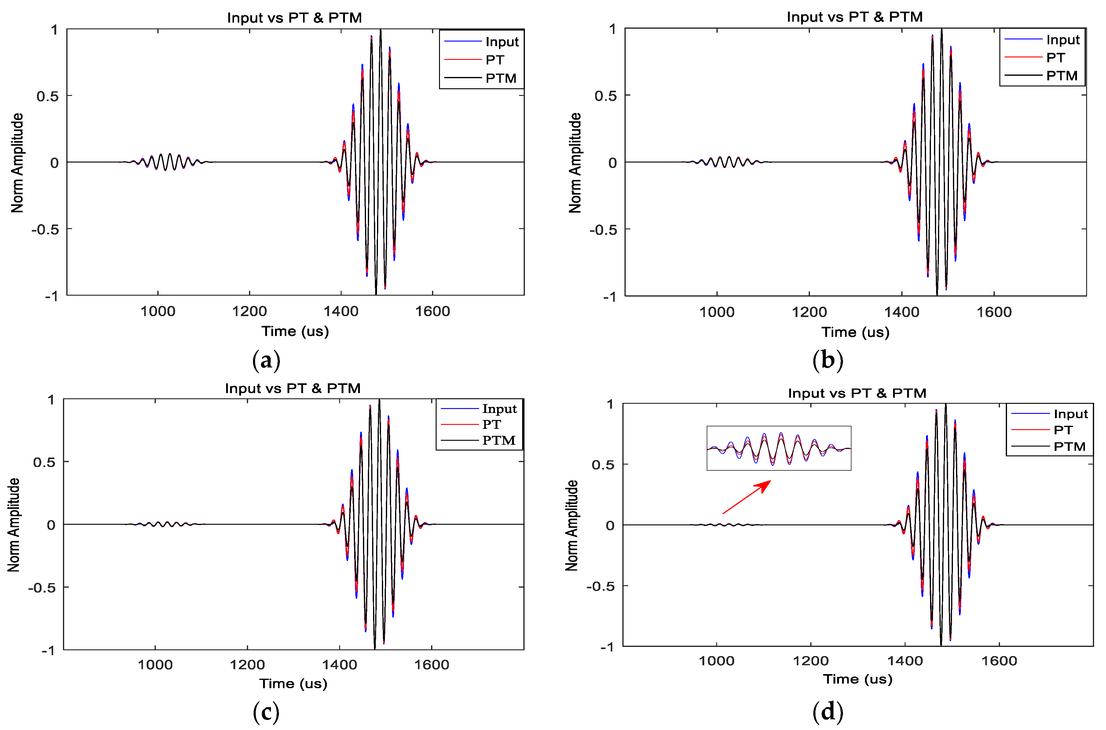
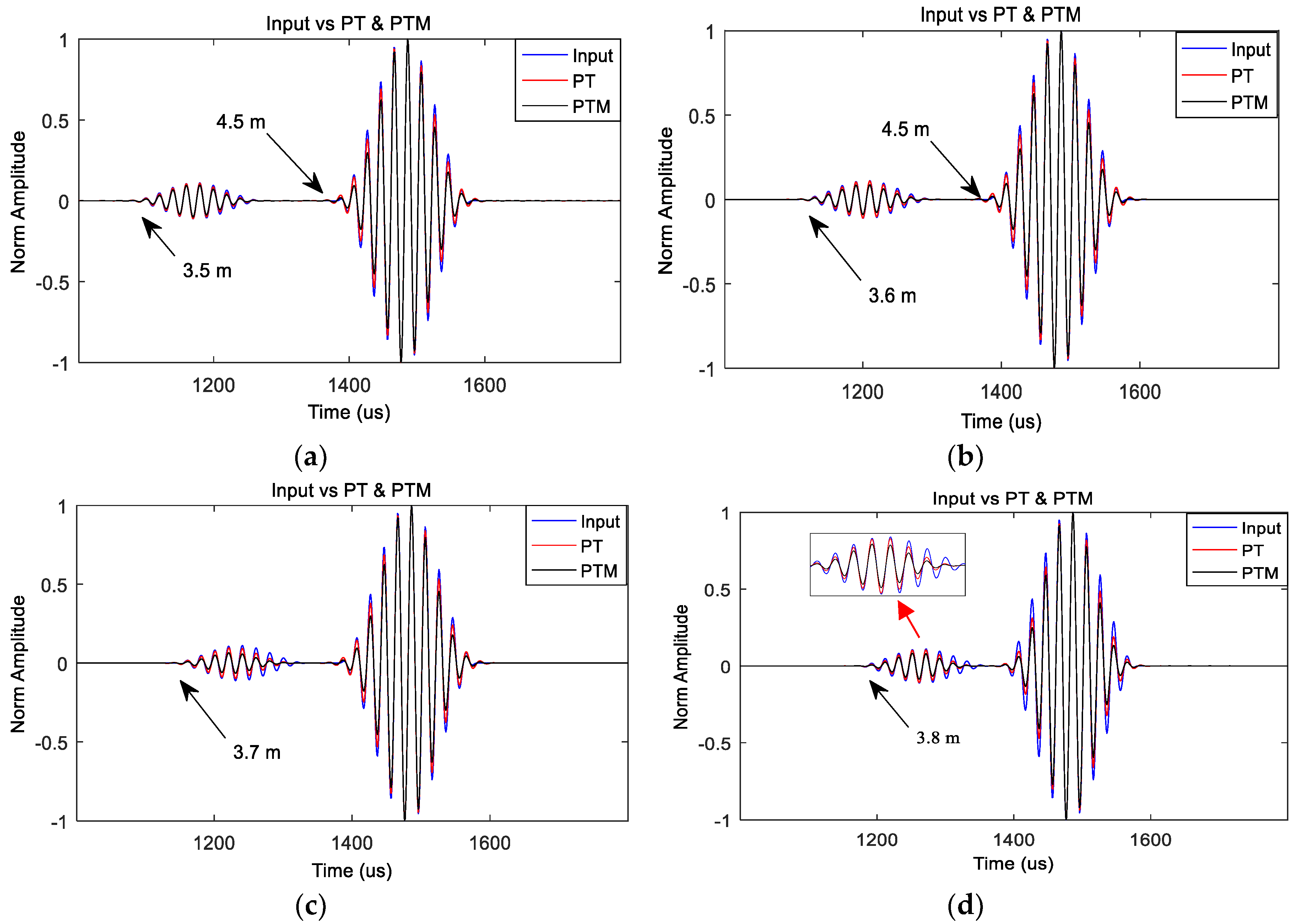
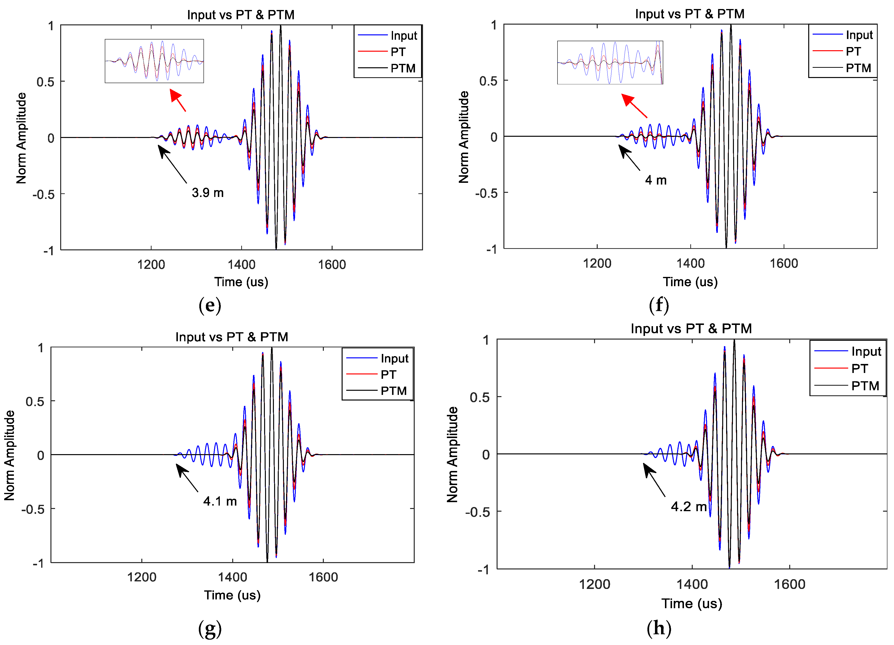
The set-up of this experiment is shown in Figure 4. The distances of the defect and pipe end are and from the excitation point, respectively. It is assumed that the defect reflects 6% of the total energy and rest of the energy (94%) is reflected by the pipe end, as displayed in Figure 5a. The reflections from the defect were reduced gradually in order to find the smallest defect size that can be recognised by the proposed method. These are illustrated in Figure 5, where the defect sizes are gradually reduced from 6% CSA to 1% CSA. The results demonstrate that the proposed method has the potential to detect defects down to 1% CSA when the distance between two features is 1.5 m. Then, in order to find the distance limitation, it is assumed that a 10% CSA defect is 1 m from the pipe end and it is moved towards the pipe end in steps of 0.1 m as illustrated in Figure 4. Results in Figure 6a–d clearly demonstrate that the defect was recognisable until the distance from the pipe end was around 0.7 m. After that, as shown in Figure 6f, the resolution was gradually reduced until it reaches 0.5 m. Afterwards, the defect reflection started to superimpose on the pipe end reflection, and it travelled below the limit of the resolution. Therefore, according to this result, SSP with the proposed parameters can detect small amplitudes that are close to the dominant amplitude only when the distance between them is greater than 0.5 m. Note that this is the result for 10 cycles of excitation signal with a defect size of 10% CSA and a centre frequency of 50 kHz.
Furthermore, as shown in Figure 6, the results of PT and PTM algorithms are almost identical while the distance between the two peaks is greater than 0.8 m. However, the PT algorithm gives a better temporal resolution when the distance is around 0.5 m (Figure 5f). In these regions, the PT identify defects partially, whereas the PTM loses the information completely, and finally, when the distance is less than 0.4 m, both algorithms miss the defect. The result of the synthesised signal showed that SSP application has the potential to reduce the level of coherent noise significantly, due to the presence of DWM, hence enhancing the SNR and the spatial resolution of signals.
In addition, a threshold (0.4 m distance between two features) was defined as a distance limitation, below which threshold the temporal resolution will be reduced. However, further work is required for the different scenarios. Furthermore, in order to validate the outcome of these synthesised results, SSP was applied to the experimental data that was gathered in the lab. These validations are described next.
4. Experimental Validation
In this section, two experiments were carried out in the laboratory to validate the proposed method for the reduction of DWM, and to enhance the spatial resolution in GWT.
4.1. Experiment #1: One Saw Cut Defect
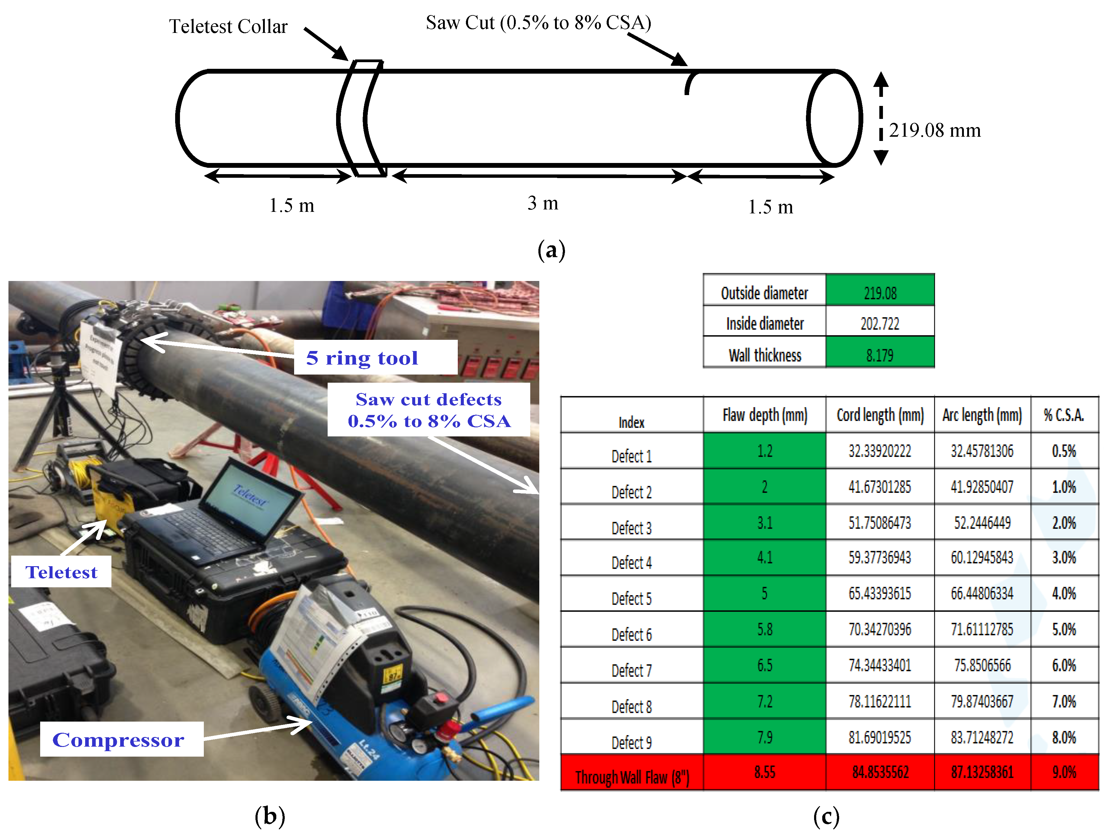
The first experiments were conducted in the lab using a nominal eight-inch steel pipe, 6 m long, with a wall thickness of 8.28 mm and an outer diameter of 219.08 mm. The setup for the experiment is illustrated in Figure 7. The signal was excited/received (Tx/Rx) using a Teletest system to transmit a 10-cycle Hann window modulated tone burst of T(0,1) wave mode. The ring spacing between the transducers was 30 mm.
The frequencies that give the best results for this particular pipe size according to the dispersion curve are 27 kHz, 36 kHz, 44 kHz, 64 kHz, and 72 kHz. Therefore, the data was collected at these frequencies for analysis. The Teletest Collar was placed at 1.5 m away from the near pipe-end, and a saw cut defect was introduced 1.5 m away from the far pipe-end. The size of the defect was incrementally increased from 0.5% CSA to 8% CSA in nine steps. The flaw size plan is displayed in Figure 7c. In order to reduce incoherent noise, the collection was repeated 512 times, and the received signals were averaged. The sampling frequency of the received signal was set to 1MHz. Since PT algorithm gave the best result for synthesised signal, it was used in this experiment with the same filter bank parameters that were employed for the synthesised signal as illustrated in Table 1.
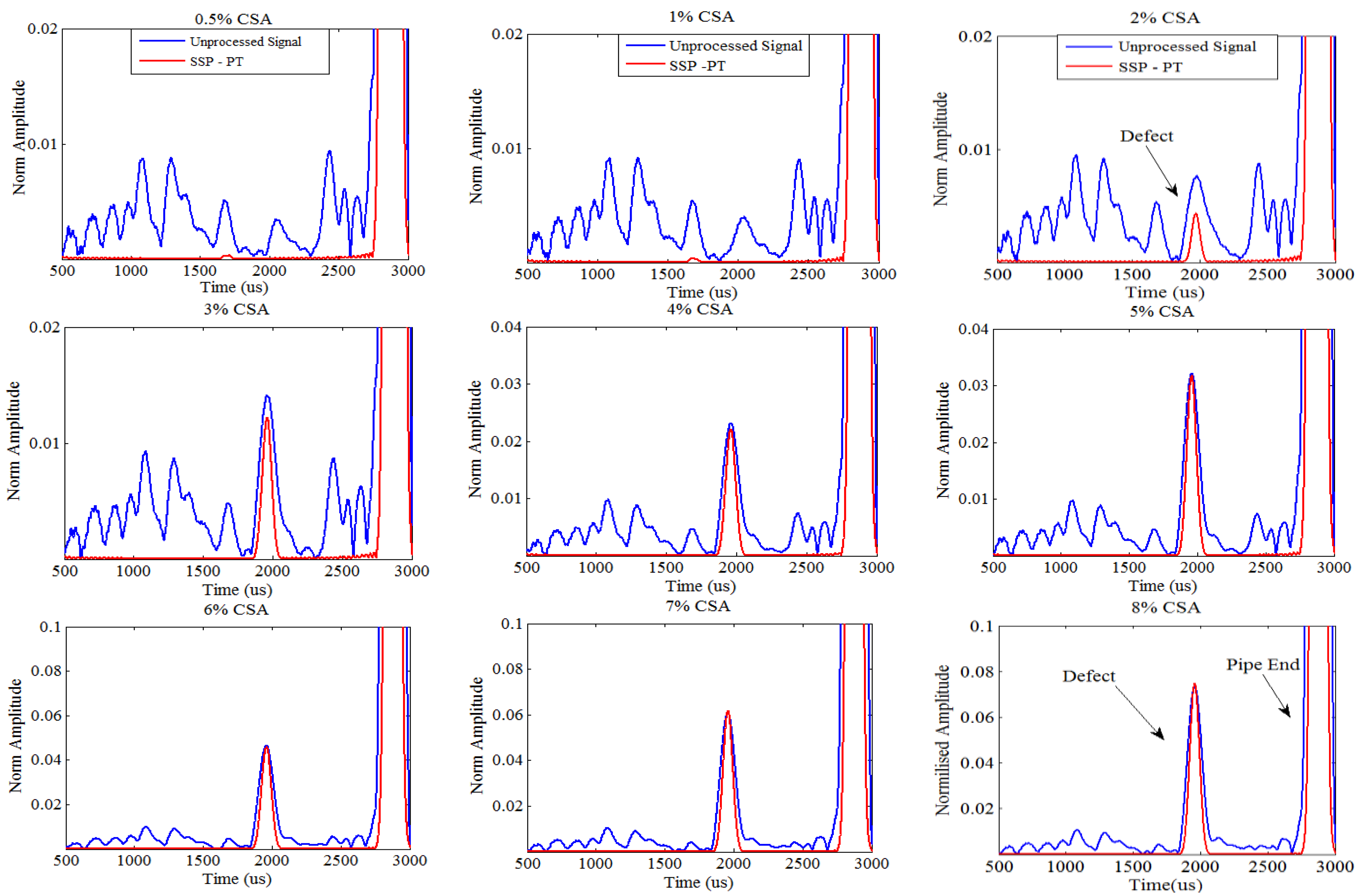
As mentioned earlier, the experiment was run for different frequencies, and the result of each frequency was compared with the conventional model that is currently employed in the Teletest system. However, the comparison for 44 kHz is presented in greater detail in this paper. The results indicated that defects that are smaller than 2% CSA are almost impossible to identify before and/or after applying the proposed technique. Therefore, the investigation and comparison were confined to when the defect size was greater than 2% CSA. It is notable that the current sensitivity for reliable detection of the Teletest system was 9% CSA, which is equivalent to 5% amplitude reflection.
Figure 8 shows the zoom-in plot around the defects area from 0.5% CSA to 8% CSA using MatLab software for both the unprocessed (blue trace) signal and the SSP (red trace) signal. The figure confirms that the SSP technique using optimum parameters enhances the defect sensitivity down to 2% CSA, which was hidden below the noise level. As shown in Figure 8, it was still difficult to identify a 3% CSA defect with the conventional techniques, whereas the proposed method removed all of the surrounding noise, and only the defect’s reflection remained. Hence, the defect was easily noticeable and it could be identified with confidence. This size flaw was typical of that which can be challenging to reliably detect with GWT systems. Therefore, as a result of this experiment, SSP demonstrates great potential to enhance the SNR, and to increase the sensitivity and spatial resolution of signal response, and it is able to identify defects down to 2% CSA.
SNR Calculation
In order to quantify the improvements shown by the proposed technique, the SNR enhancement was calculated as:
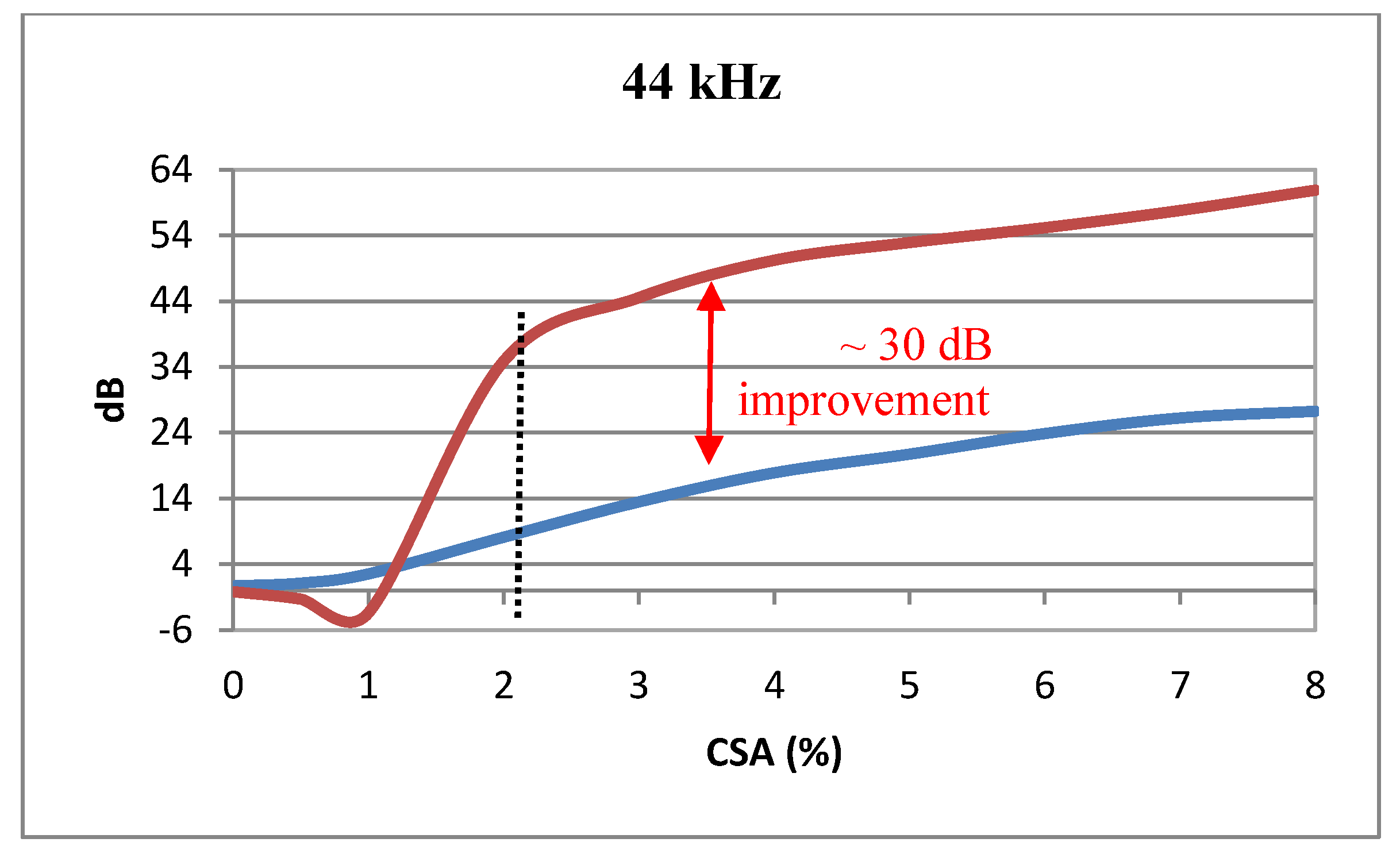
where S is the maximum amplitude of the defect’s reflection, and N is the root mean square (RMS) value of the noise region around the defect. The SNR of the unprocessed signal was 7.8 dB when the defect size was 2% CSA, and 13.25 dB when the defect size was 3% CSA. The results presented in Table 2 show that the SSP algorithms enhanced the SNR by 34.9 dB and 42.9 dB for these cases respectively. Furthermore, a comparison of the amplitude of the pipe-end reflection and the defect reflection was undertaken in order to evaluate how well the SSP maintains the amplitude of the signal of interest. The results indicate that when the size of the defect was 3% CSA or greater, there were no significant amplitude changes that occurred for the proposed method.
Figure 9 illustrates the result of the unprocessed signal (blue trace) and the SSP algorithm (red trace) for the above experiment when there was no defect (baseline), up to when the defect size was 8% CSA. The results clearly illustrated that the performance of the proposed technique massively improved the SNR of the GWT response compared to the unprocessed data, achieving around 30 dB improvement for 44 kHz. However, as mentioned earlier, the comparison commenced when the defect size was at least 2% CSA. Hence, in order to clarify it, a dotted line was added at 2% CSA.
4.2. Experiment #2: Two Saw Cut Defects
The aim of this test was to investigate the distance limitation of SSP where a small feature (i.e., defect) is close to a dominant feature (e.g., weld). The initial investigation started with the optimum parameters utilised for a single saw cut defect to evaluate the outcome of SSP distance limitation.
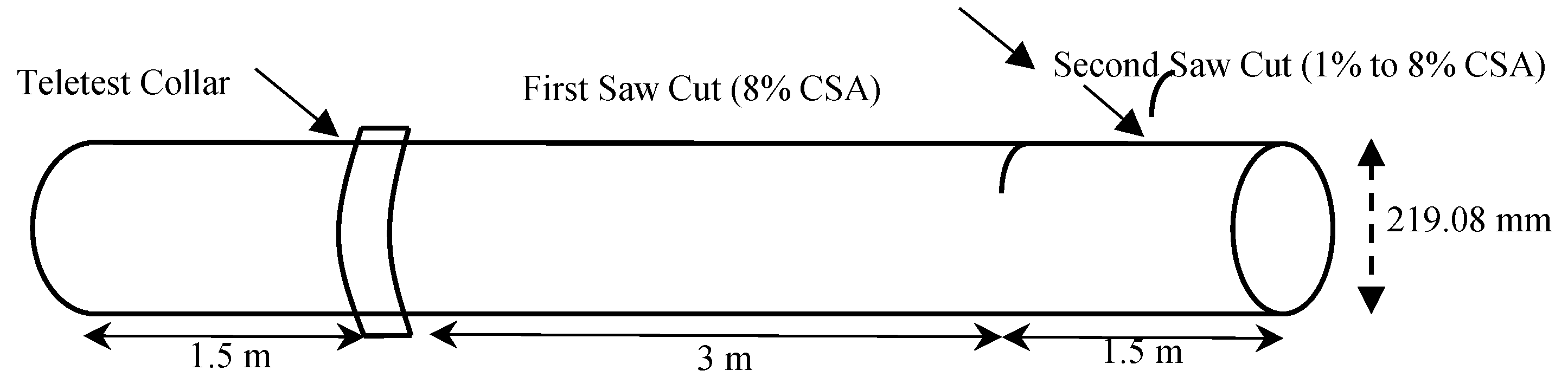
An experiment was carried out on the same eight-inch pipe that was utilised for the previous experiment. In this experiment, another saw cut defect was added to the pipe at a location that was 48 cm from the far pipe end, as shown in Figure 10. The size of the defect was incrementally increased from 1% CSA to 8% CSA. Note that another 8% CSA saw cut defect already existed 1.5 m from the far pipe end. All of the setups, the tool location, and the frequency test region were exactly the same as the previous exercise. However, only the results relating to 44 kHz were presented here because, according to the previous experiment, this frequency gave the best SNR enhancement.
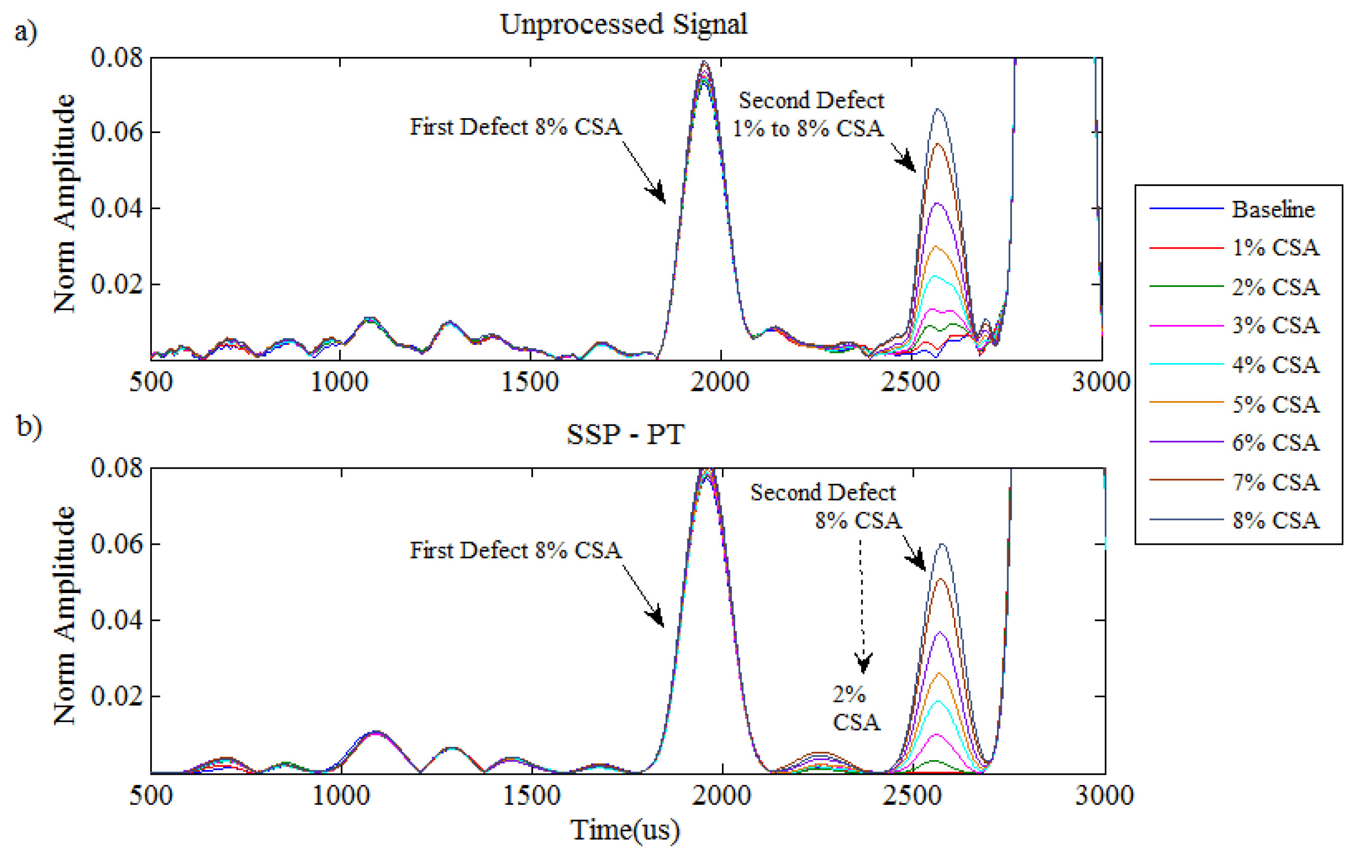
The proposed method was applied to the collected data gathered from this experiment. It was observed that the initial result obtained with these parameters was not as successful, and it was only able to identify defects down to 4% CSA. Hence, the brute force search algorithm was applied to find the optimum parameter values for this scenario, again in order to improve the performance of the defects, and the capability to find smaller defects. As a result, optimum values were discovered that gave the chance to detect defects down to 2% CSA for a second defect. The unprocessed signal, and the signal after applying SSP with the new optimum parameters are presented in Figure 11. This figure clearly demonstrates that the data after applying SSP are tidier in general, and in terms of defect detection, down to 2% CSA is noticeable. However, it can be seen that the coherent noise is hardly reduced by the new parameters, and SNR is slightly improved. Therefore, it is confirmed that there is a trade-off between detecting small features next to a dominant signal and improving the SNR. In addition, this result confirms the result of the synthesised analysis where it was stated that the distance limitation of SSP to identify adjacent features is around 50 cm when using a 10-cycle Hann windowed at 44 kHz.
4.3. Discussion
The limitations of SSP were first investigated for synthesised signals using the two most common SSP recombination algorithms, polarity thresholding (PT) and PT with minimisation (PTM). The synthesised signals were utilised to find the limitations of SSP by measuring the SNR and spatial resolution of the received signal. Results showed that the SSP with PT algorithm was able to identify defects down to 1% CSA, and stated that 50 cm is the minimum distance for the SSP to identify a defect next to the pipe end. Then, in order to validate the synthesised results, two experimental tests have been carried out in the lab on the same sized pipe.
Two experiments were carried out on an eight inch pipe, 6 m long, with a wall thickness of 8.28 mm and an outer diameter of 219.08 mm, using a pulse-echo technique. The Teletest system was utilised to transmit a 10-cycle Hann window-modulated tone burst of T(0,1) with a centre frequency of 44 kHz. In the first experiment, a saw cut defect was created 1.5 m from the far pipe-end. Nine saw cut defects were created, the sizes of which gradually increased from 0.5% CSA to 8% CSA. The results demonstrate that the SNR was improved by approximately 30 dB compared to the unprocessed signal. The results indicated that defects smaller than 2% CSA cannot be identified both before and after SSP. This is due to the sensitivity of the system. Therefore, the investigation and comparison were conducted only when the defect size was greater than 2% CSA. It was shown that the 2% CSA defect’s reflection was almost masked by the coherent noise level, and that the identification of responses using conventional signal interpretations was not feasible. However, SSP removed all the surrounding coherent noise but the defect’s reflection. Therefore, this provided a good evidence that SSP has the potential to identify defects down to 2% CSA, and to enhance the spatial resolution.
In the second experiment, a new saw cut defect was created, which varied in size from 1% CSA to 8% CSA in each test, in addition to the already existing 8% CSA defect. The aim was to validate the distance limitation that was observed for the synthesised exercise. Therefore, the defects were created 48 cm from the far pipe-end. The results illustrated that defects up to 4% CSA were detectable with the same filter bank parameters as those used for the previous scenarios. However, in terms of identifying smaller defects, the parameters needed to be modified, and this was undertaken using a brute force search algorithm. As a result, new filter bank parameters were introduced to identify defects down to 2% CSA. However, this was achieved at the cost of reducing the SNR enhancement.
The above algorithm and methodology explain a means of identifying potentially reusable parameters of SPP for the application of suppressing dispersive wave modes in GWT. It should be noted that pipes of the similar geometry and material share the same guided wave characteristics. The relative rates of dispersion between the desired/undesired wave modes will be the same for equivalent pipes. Regulation in the oil and gas sectors means that pipelines are manufactured from a limited set of standard geometries and materials. Hence, equivalent pipes are commonplace. Therefore, it is anticipated that once the set of parameters have been identified for a specific pipe, they can be reused effectively for similar or slightly different pipes. This would mean it would not be required to run the brute force search algorithm for every inspection. However, the proposed technique was tested in a limited trial, and in order to build a signal processing toolbox (automated), more field data analysis is required to be investigated.
5. Conclusions
A novel solution based on signal processing is proposed in this work to address the problem of coherent noise in guided wave testing using the SSP technique. The main concern was to identify the limitations of SSP in terms of sensitivity and resolution when two features are close to each other.
Therefore, a synthesised signal has been created to identify the limitations of SSP in terms of establishing the smallest defect that can be detected, and to establish the resolution limitation when the location of a defect is close to a dominant feature. It was demonstrated that the SSP technique with optimum parameters successfully identified defects down to 2% CSA, and enhanced the SNR of the received signal. In addition, a threshold of 50 cm has been defined, below which the temporal resolution will be significantly reduced. The outcome was then experimentally validated for an eight-inch pipe containing two saw cut defects using the Teletest system, where it achieved a comparable result. To sum up, it is demonstrated throughout this work that the proposed method using a polarity thresholding algorithm has the potential to improve the sensitivity and spatial resolution of GWT in terms of SNR (by up to 30 dB), by detecting smaller defects (down to 2% CSA) with a resolution threshold of 50 cm between the two features. Thus, this work shows that SSP, as implemented here, could be applied for pipeline inspection using the GWT technique.
Further work on this subject should focus on validation of this technique with field data, which are usually more complex and contain different types of defects. Furthermore, the sensitivity of this algorithm could be investigated for coated and buried pipelines, where the attenuation rates are sufficiently high that they cause a major reduction in guided wave test capability.
Author Contributions
S.K.P. conducted the synthesised modelling, analysis, programming, experiments, and drafted the manuscript; P.M. helped edit the manuscript; T.-H.G. contributed to reviewing the manuscript.
Funding
This research was funded by the National Structural Integrity Research Centre (NSIRC), managed by TWI with the partnership of Brunel University.
Acknowledgments
The authors gratefully acknowledge TWI and PI Ltd. for granting access to the Teletest equipment.
Conflicts of Interest
The authors declare no conflict of interest.
References
- Rose, J.L. An introduction to ultrasonic guided waves. In Proceedings of the 4th Middle East NDT Conference and Exhibition, Manama, Bahrain, 2–5 December 2007. [Google Scholar]
- Rose, J.L. Ultrasonic guided waves in structural health monitoring. Key Eng. Mater. 2004, 270–273, 14–21. [Google Scholar] [CrossRef]
- Catton, P. Long Range Ultrasonic Guided Waves for the Quantitative Inspection of Pipelines. Ph.D. Thesis, Brunel University, Uxbridge, UK, 2009. [Google Scholar]
- Fateri, S.; Lowe, P.S.; Engineer, B.; Boulgouris, N.V. Investigation of ultrasonic guided waves interacting with piezoelectric transducers. IEEE Sens. J. 2015, 15, 4319–4328. [Google Scholar] [CrossRef]
- Mallett, R.; Mudge, P.; Gan, T.; Balachandra, W. Analysis of cross-correlation and wavelet de-noising for the reduction of the effects of dispersion in long-range ultrasonic testing. Insight-Non-Destr. Test. Cond. Monit. 2007, 49, 350–355. [Google Scholar] [CrossRef]
- Wilcox, P.; Lowe, M.; Cawley, P. The effect of dispersion on long-range inspection using ultrasonic guided waves. NDT E Int. 2001, 34, 1–9. [Google Scholar] [CrossRef]
- Wilcox, P.D. A rapid signal processing technique to remove the effect of dispersion from guided wave signals. IEEE Trans. Ultrason. Ferroelectr. Freq. Control 2003, 50, 419–427. [Google Scholar] [CrossRef] [PubMed]
- Zeng, L.; Lin, J. Chirp-based dispersion pre-compensation for high resolution Lamb wave inspection. NDT E Int. 2014, 61, 35–44. [Google Scholar] [CrossRef]
- Xu, K.; Ta, D.; Moilanen, P.; Wang, W. Mode separation of Lamb waves based on dispersion compensation method. J. Acoust. Soc. Am. 2012, 131, 714–722. [Google Scholar] [CrossRef] [PubMed]
- Xu, K.; Ta, D.; Hu, B.; Laugier, P.; Wang, W. Wideband dispersion reversal of lamb waves. IEEE Trans. Ultrason. Ferroelectr. Freq. Control 2014, 61, 997–1005. [Google Scholar] [CrossRef] [PubMed]
- Xu, K.; Liu, C.; Ta, D. Ultrasonic guided waves dispersion reversal for long bone thickness evaluation: A simulation study. In Proceedings of the 2013 35th Annual International Conference of the IEEE Engineering in Medicine and Biology Society (EMBC), Osaka, Japan, 3–7 July 2013; pp. 1930–1933. [Google Scholar]
- Toiyama, K.; Hayashi, T. Pulse compression technique considering velocity dispersion of guided wave. Rev. Prog. Quan. Nondestr. Eval. 2008, 975, 587–593. [Google Scholar]
- Yucel, M.; Fateri, S.; Legg, M.; Wilkinson, A.; Kappatos, V.; Selcuk, C.; Gan, T.-H. Coded Waveform Excitation for High Resolution Ultrasonic Guided Wave Response. IEEE Trans. Ind. Inform. 2016, 12, 257–266. [Google Scholar] [CrossRef]
- Yucel, M.; Fateri, S.; Legg, M.; Wilkinson, A.; Kappatos, V.; Selcuk, C.; Gan, T.-H. Pulse-compression based iterative time-of-flight extraction of dispersed ultrasonic guided waves. In Proceedings of the 2015 IEEE 13th International Conference on Industrial Informatics (INDIN), Cambridge, UK, 22–24 July 2015; pp. 809–815. [Google Scholar]
- Newhouse, V.; Bilgutay, N.; Saniie, J.; Furgason, E. Flaw-to-grain echo enhancement by split-spectrum processing. Ultrasonics 1982, 20, 59–68. [Google Scholar] [CrossRef]
- Karpur, P.; Shankar, P.; Rose, J.; Newhouse, V. Split spectrum processing: Optimizing the processing parameters using minimization. Ultrasonics 1987, 25, 204–208. [Google Scholar] [CrossRef]
- Shankar, P.M.; Karpur, P.; Newhouse, V.L.; Rose, J.L. Split-spectrum processing: Analysis of polarity threshold algorithm for improvement of signal-to-noise ratio and detectability in ultrasonic signals. Trans. Ultrason. Ferroelectr. Freq. Control 1989, 36, 101–108. [Google Scholar] [CrossRef] [PubMed]
- Saniie, J.; Oruklu, E.; Yoon, S. System-on-chip design for ultrasonic target detection using split-spectrum processing and neural networks. Trans. Ultrason. Ferroelectr. Freq. Control 2012, 59, 1354–1368. [Google Scholar] [CrossRef] [PubMed]
- Gustafsson, M.G.; Stepinski, T. Adaptive split spectrum processing using a neural network. Res. Nondestruct. Eval. 1993, 5, 51–70. [Google Scholar] [CrossRef]
- Gustafsson, M.G. Towards adaptive split spectrum processing. IEEE Ultrason. Symp. 1995, 1, 729–732. [Google Scholar]
- Rubbers, P.; Pritchard, C.J. Complex plane Split Spectrum Processing: An introduction. NDT Net 2003, 8, 1–8. [Google Scholar]
- Rubbers, P.; Pritchard, C.J. An overview of Split Spectrum Processing. J. Nondestruct. Test. 2003, 8, 1–11. [Google Scholar]
- Rodríguez, A. A new filter bank design for split-spectrum algorithm. NDT 2009, 1, 1–7. [Google Scholar]
- Rodriguez, A.; Miralles, R.; Bosch, I.; Vergara, L. New analysis and extensions of split-spectrum processing algorithms. NDT E Int. 2012, 45, 141–147. [Google Scholar] [CrossRef]
- Syam, G.; Sadanandan, G.K. Flaw Detection using Split Spectrum Technique. Int. J. Adv. Res. Electr. Electron. Instrum. Eng. 2014, 3, 8118–8127. [Google Scholar]
- Pedram, S.K.; Fateri, S.; Gan, L.; Haig, A.; Thornicroft, K. Split-Spectrum Processing Technique for SNR Enhancement of Ultrasonic Guided Wave. Ultrasonics 2018, 83, 48–59. [Google Scholar] [CrossRef] [PubMed]
- Eddyfi Ltd. 2018. Available online: http://www.teletestndt.com/ (accessed on 10 July 2018).
- Beasley, H.R.; Eric, W. A Quantitative Analysis of Sea Clutter Decorrelation with Frequency Agility. IEEE Trans. Aerosp. Electron. Syst. 1968, 4, 468–473. [Google Scholar] [CrossRef]
- Pedram, S.; Haig, A.; Lowe, P.; Thornicroft, K.; Gan, L.; Mudge, P. Split-Spectrum Signal Processing for Reduction of the Effect of Dispersive Wave Modes in Long-range Ultrasonic Testing. Phys. Procedia 2015, 70, 388–392. [Google Scholar] [CrossRef]
- Pavlakovic, B.; Lowe, M.; Alleyne, D.; Cawley, P. Disperse: A general purpose program for creating dispersion curves. In Review of Progress in Quantitative NDE; Springer: New York, NY, USA, 1997; pp. 185–192. [Google Scholar]
- Bottger, W.; Schneider, H.; Weingarten, W. Prototype EMAT system for tube inspection with guided ultrasonic waves. Nucl. Eng. Des. 1987, 102, 369–376. [Google Scholar] [CrossRef]
Figure 1.
guided wave testing (GWT) signals: an excitation (a) time domain and (b) frequency domain signal, received (c) time domain and (d) frequency domain signal.
Figure 1.
guided wave testing (GWT) signals: an excitation (a) time domain and (b) frequency domain signal, received (c) time domain and (d) frequency domain signal.

Figure 2.
Split-spectrum processing (SSP) block diagram.

Figure 3.
Filter bank parameters of SSP.

Figure 4.
Synthesised setup for an eight inch pipe with a wall thickness of 8.179 mm and an outside diameter of 219.08 mm.
Figure 4.
Synthesised setup for an eight inch pipe with a wall thickness of 8.179 mm and an outside diameter of 219.08 mm.

Figure 5.
Results for the synthesised signal before and after applying SSP ((polarity thresholding & Polarity thresholding with minimisation)PT & PTM). The defect and the pipe end are located at X = 3 m and X = 4.5 m from the excitation signal. The defect sizes are (a) 6% cross-section area (CSA); (b) 4% CSA; (c) 2% CSA; and (d) 1% CSA.

Figure 6.
Results for the synthesised signal before and after applying SSP (PT & PTM). The defect (X = 3.5 m) is moved towards the pipe end (X = 4.5 m) in steps of 0.1 m. The defect distances are X= (a) 3.5 m; (b) 3.6 m; (c) 3.7 m; (d) 3.8 m; (e) 3.9 m; (f) 4 m; (g) 4.1 m; (h) 4.2 m.
Figure 6.
Results for the synthesised signal before and after applying SSP (PT & PTM). The defect (X = 3.5 m) is moved towards the pipe end (X = 4.5 m) in steps of 0.1 m. The defect distances are X= (a) 3.5 m; (b) 3.6 m; (c) 3.7 m; (d) 3.8 m; (e) 3.9 m; (f) 4 m; (g) 4.1 m; (h) 4.2 m.


Figure 7.
Experimental setup up for an eight inch steel pipe with a wall thickness of 8.179 mm and an OD of 219.08 mm (a,b), and (c) its flaw size plan.
Figure 7.
Experimental setup up for an eight inch steel pipe with a wall thickness of 8.179 mm and an OD of 219.08 mm (a,b), and (c) its flaw size plan.

Figure 8.
Zoom in around the defect area from 0.5% CSA up to 8% CSA.

Figure 9.
SNR calculation–peak amplitude of the defect (S) to the root mean square (RMS) value of the noise region (N) for 44 kHz.
Figure 9.
SNR calculation–peak amplitude of the defect (S) to the root mean square (RMS) value of the noise region (N) for 44 kHz.

Figure 10.
Experimental setup for the same eight inch pipe (Figure 7) with two saw cut defects.
Figure 10.
Experimental setup for the same eight inch pipe (Figure 7) with two saw cut defects.

Figure 11.
Zoom in result with two defects. (a) Unprocessed signal; (b) SSP signal.


Table 1.
Recommended values for SSP parameters.
| SSP Parameters | Symbols | Recommended Values |
|---|---|---|
| Total bandwidth | 99% of total energy | |
| Sub-band filter bandwidth | ||
| Filter crossover point | ||
| Filter separation | 1 dB | |
| Number of filters |
Table 2.
Signal-to-noise ratio (SNR) enhancement of experimental signal.
| Signal | 2% Defect | 3% Defect |
|---|---|---|
| SSP | 34.9 dB | 42.9 dB |
| Unprocessed | 7.8 dB | 13.3 dB |
© 2018 by the authors. Licensee MDPI, Basel, Switzerland. This article is an open access article distributed under the terms and conditions of the Creative Commons Attribution (CC BY) license (http://creativecommons.org/licenses/by/4.0/).
Share and Cite
MDPI and ACS Style
Pedram, S.K.; Mudge, P.; Gan, T.-H. Enhancement of Ultrasonic Guided Wave Signals Using a Split-Spectrum Processing Method. Appl. Sci. 2018, 8, 1815. https://doi.org/10.3390/app8101815
AMA Style
Pedram SK, Mudge P, Gan T-H. Enhancement of Ultrasonic Guided Wave Signals Using a Split-Spectrum Processing Method. Applied Sciences. 2018; 8(10):1815. https://doi.org/10.3390/app8101815
Chicago/Turabian StylePedram, Seyed Kamran, Peter Mudge, and Tat-Hean Gan. 2018. "Enhancement of Ultrasonic Guided Wave Signals Using a Split-Spectrum Processing Method" Applied Sciences 8, no. 10: 1815. https://doi.org/10.3390/app8101815
Note that from the first issue of 2016, this journal uses article numbers instead of page numbers. See further details here.