Secure Multiple-Input Multiple-Output Communications Based on F–M Synchronization of Fractional-Order Chaotic Systems with Non-Identical Dimensions and Orders

Abstract

This paper investigates the $\mathbf{F}$–$\mathbf{M}$ synchronization between non-identical fractional-order systems characterized by different dimensions and different orders. $\mathbf{F}$–$\mathbf{M}$ synchronization combines the inverse generalized synchronization with the matrix projective synchronization. In particular, the proposed approach enables the $\mathbf{F}$–$\mathbf{M}$ synchronization to be achieved between an n-dimensional master system and an m-dimensional slave system. The developed approach is applied to chaotic and hyperchaotic fractional systems with the aim of illustrating its applicability and suitability. A multiple-input multiple-output (MIMO) secure communication system is also developed by using the $\mathbf{F}$–$\mathbf{M}$ synchronization and verified through computer simulations.

1. Introduction

Synchronization is the process of controlling the output of a chaotic dynamical slave system in order to force its variables to match those of a corresponding master system in time [1]. The subject of synchronization has been around for about 30 years. Over the course of this period, the subject has attracted the interest of researchers from a variety of fields including but not limited to engineering, natural sciences, social sciences, physics, chemistry, and many more. Although the amount of literature related to chaotic dynamical systems is vast, an exact definition of such systems is not easy to find. The general consensus, however, is that a chaotic system is one with an extremely high sensitivity to small variations in the initial conditions. The trajectory of the solutions is seemingly random and difficult to pretend. However, if the initial conditions are known, the trajectory can be exactly reproduced. Chaotic systems and their synchronization are of particular interest in the field of secure communications due to the many similarities between chaos and the encryption of data being transmitted.

Synchronization in general requires some form of control strategy. Various kinds of control schemes can be found in the literature aimed at synchronizing integer-order chaotic systems [2]. However, most of the existing studies consider only the simple case where both systems have exact same order and the same dimensions. Attempts have been dedicated to synchronize systems with different dimensions such as those shown in Table 1. The importance of different dimensional dynamic system synchronization stems from its wide range of applications as well as its enrichment of control theory.

Table 1. Synchronization schemes for integer-order systems with different dimensions.

Synchronization Schemes
Inverse full state hybrid projective synchronization [3]
Matrix projective synchronization [4].
Generalized synchronization [5].
Inverse generalized synchronization [6].
Hybrid synchronization [7].
$\mathsf{\Phi }$–$\mathsf{\Theta }$ synchronization [8].
Q–S synchronization [9].
Reduced order synchronization [10].
Increased order generalized synchronization [11].

In addition to integer-order systems, the research community has also been looking at fractional-order ones due to the added flexibility chaotic nature which they add to the mix [12]. The same progress made with integer-order systems has been attempted here. Some studies have examined the synchronization of fractional-order systems with identical dimensions [13] and others considered the more general case of arbitrary dimensions [14,15].

This study presents a novel contribution to the topic. We investigate $\mathbf{F}$–$\mathbf{M}$ synchronization, which combines generalized synchronization based on a functional relationship $\mathbf{F}$ with inverse matrix projective synchronization based on a matrix $\mathbf{M}$ with synchronization index d, which basically represents the dimension of the synchronization error. By exploiting the fractional Laplace transform along with the stability theory related to linear systems with integer orders, the $\mathbf{F}$–$\mathbf{M}$ synchronization of fractional-order systems is proven for the case $d=m$ showing that the zero solution of the error system is globally asymptotically stable. The case $d<m$ is also considered and the synchronization demonstrated. The proposed scheme is rather general with the only restriction on the scaling functions being that they must be differentiable.

Chaos has attracted considerable attention in the field of wireless and optical communications over the last two decades. The main reason for this attraction is the many similarities between chaos and encryption, which is a necessary part of any modern communications system [16,17]. Traditionally, encryption was performed at higher layers within the Open Systems Interconnection (OSI) communications model. With chaos, security concerns have shifted to the physical layer where the carriers of information, which were always sine and cosine waves, are replaced with chaotic or hyperchaotic signals. The amount of literature concerning the use of chaos in communications is vast [18]. However, they may be generally classified into five main categories: masking schemes, modulations schemes, multiple access schemes, multicarrier schemes, and secret/public key encryption schemes. In this paper, we employ the proposed $\mathbf{F}$–$\mathbf{M}$ synchronization strategy to form a multiple input multiple output (MIMO) secure communications system based on message masking. The developed system is tested through numerical simulations to verify its validity.

In the next section of this paper, we will start by defining the required fractional operators and their Laplace transforms. We then formulate the $\mathbf{F}$–$\mathbf{M}$ synchronization problem with index d. In Section 3, we present two different theorems that cover the two distinct synchronization cases with $d=m$ and $d<m$, respectively. Finally, in order to show the applicability of the developed schemes, Section 4 considers the $\mathbf{F}$–$\mathbf{M}$ synchronization of a three-dimensional fractional chaotic system and a four-dimensional fractional hyperchaotic system subject to synchronization indices $d=4$, $d=3$, and $d=2$. Section 5 presents the proposed MIMO communications system based on $\mathbf{F}$–$\mathbf{M}$ synchronization along with simulation results. Finally, concluding remarks are given in Section 6.

2. Problem Formulation

Before posing our synchronization problem and establishing its control strategy, let us first recall some of the required definitions. Let us denote the Riemann–Liouville fractional integral operator [19] and the Caputo fractional derivative [20] of a function $f\left(t\right)$ for $t>0$, respectively, by

$$J^{p}f\left(t\right)=\frac{1}{\mathsf{\Gamma }\left(p\right)}{\int }_0^t{(t-\tau )}^{p-1}f\left(\tau \right)d\tau ,p>0,$$

(1)

and

$$D_t^{p}f\left(t\right)=J^{m-p}\left(\frac{d^m}{d{t}^m}f\left(t\right)\right)=\frac{1}{\mathsf{\Gamma }(m-p)}{\int }_0^t\frac{f^{\left(m\right)}\left(\tau \right)}{{(t-\tau )}^{p-m+1}}d\tau ,m-1<p\le m,m\in IN.$$

(2)

As defined in [21], the Laplace transform of the Riemann–Liouville operator (1) is given by

$$\mathbf{L}\left\{J^{q}f\left(t\right)\right\}=s^{-q}F\left(s\right),\left(q>0\right).$$

(3)

Similarly, according to [22], the Laplace transform of $D_t^{p}f\left(t\right)$ is defined as

$$\mathbf{L}\left\{D_t^{p}f\left(t\right)\right\}=s^{p}F\left(s\right)-\sum _{k=0}^{n-1}{s}^{\alpha -k-1}{f}^{\left(k\right)}\left(0\right),$$

(4)

for $p>0$ and$n-1<p\le n$. Obviously, if $p\in (0,1]$, then Label (4) simplifies to

$$\mathbf{L}\left\{D_t^{p}f\left(t\right)\right\}=s^{p}F\left(s\right)-s^{p-1}f\left(0\right).$$

One of the interesting properties of the Caputo fractional derivative $D_t^p$, which will come in handy in our study [23] is the fact that subject to $f\left(t\right)$ having a continuous $k^{\mathrm{th}}$ derivative on $[0,t]$ for $k\in N$ and $t>0$, then by choosing $p,q>0$ in a way that there exists $\ell \in N$ satisfying

$$D_t^p{D}_t^{q}f\left(t\right)=D_t^{p+q}f\left(t\right),$$

(5)

with $\ell \le k$ and $p+q\in [\ell -1,\ell ]$. It is very important to note that the existence of ℓ is essential for this property to hold. For the purpose of our study, we choose p and q in the interval$\left[0,1\right[$ with $p+q\in \left]0,1\right]$, for which Label (5) is satisfied.

With these definitions in mind, let us now consider as master–slave pair the general chaotic systems

$$\left\{\begin{array}{c}{D}_t^{p}X\left(t\right)=f\left(X\left(t\right)\right),\hfill \\ D_t^{q}Y\left(t\right)=BY\left(t\right)+g\left(Y\left(t\right)\right)+U,\hfill \end{array}\right.$$

(6)

where $X\left(t\right)\in {\mathbb{R}}^n$ and $Y\left(t\right)\in {\mathbb{R}}^m$ are the master and slave state vectors, respectively, $0<p<1$, $f:{\mathbb{R}}^n\to {\mathbb{R}}^n$, $U={\left(u_i\right)}_{1\le i\le m}$ is a vector controller, and $B\in {\mathbb{R}}^{m\times m}$ and $g:{\mathbb{R}}^m\to {\mathbb{R}}^m$ are the linear and nonlinear parts of the slave system, respectively. In this paper, we are concerned with the rather general $\mathbf{F}$–$\mathbf{M}$ synchronization, which encompasses multiple types of synchronization as will be explained in the following definition and the remark thereafter.

Definition 1.

The maste-slave pair (6) is said to be $\mathbf{F}$–$\mathbf{M}$ synchronized with dimension d if there exists a controller $U={\left(u_i\right)}_{1\le i\le m}$, a differentiable function $\mathbf{F}:{\mathbb{R}}^m\to {\mathbb{R}}^d$, and a function matrix $\mathbf{M}\left(t\right)={\left(\mathbf{M}{\left(t\right)}_{ij}\right)}_{d\times n}$ such that

$$\underset{t\to +\infty }{lim}∥e\left(t\right)=\mathbf{F}\left(Y\left(t\right)\right)-\mathbf{M}\left(t\right)X\left(t\right)∥=0.$$

(7)

Remark 1.

Depending on the pair $\left(\mathbf{F}\left(.\right),\mathbf{M}\right)$, different synchronization types may arise:

(i) 

Complete synchronization for $\left(\mathbf{F}\left(.\right),\mathbf{M}\right)=\left(I,X\left(t\right)\right)$.

(ii) 

Anti–synchronization for $\left(\mathbf{F}\left(.\right),\mathbf{M}\right)=\left(I,-X\left(t\right)\right)$.

(iii) 

Matrix projective synchronization for $\left(\mathbf{F}\left(.\right),\mathbf{M}\right)=\left(I,\mathbf{M}\left(t\right)\right)$.

(iv) 

Inverse generalized synchronization for $\left(\mathbf{F}\left(.\right),\mathbf{M}\right)=\left(\mathbf{F}\left(Y\left(t\right)\right),I\right)$.

3. $\mathbf{F}$–$\mathbf{M}$ Synchronization

Establishing the control laws of the proposed $\mathbf{F}$–$\mathbf{M}$ will be tackled in two main steps. First, we look at the simpler case where the dimension d is equal to the dimension of the slave. Then, we move to prove the existence of a control law guaranteeing synchronization for cases where $d<m$.

3.1. Case 1: $d=m$

Let us start by defining the error system between the master and slave systems in Label (6) for the $\mathbf{F}$–$\mathbf{M}$ synchronization of dimension m as

$$e\left(t\right)=\mathbf{F}\left(Y\left(t\right)\right)-\mathbf{M}\left(t\right)X\left(t\right).$$

(8)

By defining the matrix

$$\mathbf{DF}\left(Y\left(t\right)\right)=\left(\begin{array}{cccc}\frac{\partial {\mathbf{F}}_1}{\partial y_1}& \frac{\partial {\mathbf{F}}_1}{\partial y_2}& \cdots & \frac{\partial {\mathbf{F}}_1}{\partial y_m}\\ \frac{\partial {\mathbf{F}}_2}{\partial y_1}& \frac{\partial {\mathbf{F}}_2}{\partial y_2}& \cdots & \frac{\partial {\mathbf{F}}_2}{\partial y_m}\\ ⋮& ⋮& \ddots & ⋮\\ \frac{\partial {\mathbf{F}}_m}{\partial y_1}& \frac{\partial {\mathbf{F}}_m}{\partial y_2}& \cdots & \frac{\partial {\mathbf{F}}_m}{\partial y_m}\end{array}\right),$$

(9)

we may reformulate (8) as

$$\dot{e}\left(t\right)=\mathbf{DF}\left(Y\left(t\right)\right)\dot{Y}\left(t\right)-\dot{\mathbf{M}}\left(t\right)X\left(t\right)-\mathbf{M}\left(t\right)\dot{X}\left(t\right).$$

(10)

It was shown in [24] that the fractional derivative of the product $\mathbf{M}\left(t\right)\dot{X}\left(t\right)$, for instance, results in an infinite sum containing integer and fractional order derivatives. Hence, we may not use Label (10) directly. Instead, let us rewrite it in the more convenient form

$$\dot{e}\left(t\right)=\left(B-C\right)e\left(t\right)+\mathbf{DF}\left(Y\left(t\right)\right)\dot{Y}\left(t\right)+R,$$

(11)

with $C\in {\mathbb{R}}^{m\times m}$ being our new constant control matrix to be selected later and

$$R=\left(C-B\right)e\left(t\right)-\dot{\mathbf{M}}\left(t\right)X\left(t\right)-\mathbf{M}\left(t\right)\dot{X}\left(t\right).$$

(12)

To achieve synchronization between the systems in Label (6), we assume that $\mathbf{DF}\left(Y\left(t\right)\right)$ is an invertible matrix with its inverse denoted by ${\mathbf{D}}^{-1}$. This leads us to the following theorem.

Theorem 1.

There exists a suitable feedback gain matrix $C\in {\mathbb{R}}^{m\times m}$ such that

$$U=-BY\left(t\right)-g\left(Y\left(t\right)\right)+J^{1-q}\left(-{\mathbf{D}}^{-1}\times R\right),$$

(13)

whereby m–dimensional $\mathbf{F}$–$\mathbf{M}$ synchronization is realized for the master–slave pair (6).

Proof. 

Substituting the control law (13) into the slave system yields

$$D_t^{q}Y\left(t\right)=J^{1-q}\left(-{\mathbf{D}}^{-1}\times R\right).$$

(14)

If we use the notation $F\left(s\right)=\mathbf{L}\left(Y\left(t\right)\right)$, the Laplace transform of (14) results in

$$s^{q}F\left(s\right)-s^{q-1}Y\left(0\right)=s^{q-1}\mathbf{L}\left(-{\mathbf{D}}^{-1}\times R\right).$$

(15)

Then, by multiplying Label (15) by $s^{1-q}$ and taking the inverse Laplace transform, we obtain

$$\dot{Y}\left(t\right)=-{\mathbf{D}}^{-1}\times R,$$

(16)

which when substituted in the error Equation (11) gives us

$$\begin{array}{ccc}\hfill \dot{e}\left(t\right)& =& \left(B-C\right)e\left(t\right)+\mathbf{DF}\left(Y\left(t\right)\right)\left[-{\mathbf{D}}^{-1}\times R\right]+R\hfill \\ & =& \left(B-C\right)e\left(t\right).\hfill \end{array}$$

(17)

The rest is simple. We can choose an arbitrary control matrix C such that all eigenvalues of $B-C$ have negative real parts, thereby guaranteeing the convergence of the error to zero, i.e., $\underset{t⟶+\infty }{lim}∥e\left(t\right)∥=0$. Consequently, we can say that the zero solution of the error system (17) is globally asymptotically stable, and thus the master–slave pair (6) is globally $\mathbf{F}$–$\mathbf{M}$ synchronized with dimension m. ☐

3.2. Case 2: $d<m$

Let us now assume that the synchronization dimension $d<m$. We define the vectors ${\dot{Y}}_1\left(t\right)={\left({\dot{y}}_1\left(t\right),...,{\dot{y}}_d\left(t\right)\right)}^T$ and ${\dot{Y}}_2\left(t\right)={\left({\dot{y}}_{d+1}\left(t\right),...,{\dot{y}}_m\left(t\right)\right)}^T$ along with matrices

$${\mathbf{D}}_1=\left(\begin{array}{cccc}\frac{\partial {\mathbf{F}}_1}{\partial y_1}& \frac{\partial {\mathbf{F}}_1}{\partial y_2}& \cdots & \frac{\partial {\mathbf{F}}_1}{\partial y_d}\\ \frac{\partial {\mathbf{F}}_2}{\partial y_1}& \frac{\partial {\mathbf{F}}_2}{\partial y_2}& \cdots & \frac{\partial {\mathbf{F}}_2}{\partial y_d}\\ ⋮& ⋮& \ddots & ⋮\\ \frac{\partial {\mathbf{F}}_d}{\partial y_1}& \frac{\partial {\mathbf{F}}_d}{\partial y_2}& \cdots & \frac{\partial {\mathbf{F}}_d}{\partial y_d}\end{array}\right),$$

(18)

$${\mathbf{D}}_2=\left(\begin{array}{cccc}\frac{\partial {\mathbf{F}}_1}{\partial y_{d+1}}& \frac{\partial {\mathbf{F}}_1}{\partial y_{d+2}}& \cdots & \frac{\partial {\mathbf{F}}_1}{\partial y_m}\\ \frac{\partial {\mathbf{F}}_{d+2}}{\partial y_{d+1}}& \frac{\partial {\mathbf{F}}_{d+2}}{\partial y_{d+2}}& \cdots & \frac{\partial {\mathbf{F}}_{d+2}}{\partial y_m}\\ ⋮& ⋮& \ddots & ⋮\\ \frac{\partial {\mathbf{F}}_d}{\partial y_{d+1}}& \frac{\partial {\mathbf{F}}_d}{\partial y_{d+2}}& \cdots & \frac{\partial {\mathbf{F}}_d}{\partial y_m}\end{array}\right),$$

(19)

and

$$T=\mathrm{diag}\left(c_1,c_2,...,c_d\right)e\left(t\right)-\dot{\mathbf{M}}\left(t\right)X\left(t\right)-\mathbf{M}\left(t\right)\dot{X}\left(t\right).$$

(20)

The error system (8) may be rearranged to the form

$$\dot{e}\left(t\right)=-\mathrm{diag}\left(c_1,c_2,...,c_d\right)e\left(t\right)+{\mathbf{D}}_1{\dot{Y}}_1\left(t\right)+{\mathbf{D}}_2{\dot{Y}}_2\left(t\right)+T,$$

(21)

where $c_i$ are positive control constants for $1\le i\le d$. We assume that matrix ${\mathbf{D}}_1$ is invertible and we denote its inverse by ${\mathbf{D}}_1^{-1}$. The following theorem states the control laws for the $\mathbf{F}$–$\mathbf{M}$ synchronization criterion.

Theorem 2.

Given the four matrices $B_1={\left(b_{ij}\right)}_{d\times m}$, $B_2={\left(b_{ij}\right)}_{\left(m-d\right)\times m}$, $G_1={\left(g_i\right)}_{1\le i\le d}$, and $G_2={\left(g_i\right)}_{d+1\le i\le m}$, the master–slave pair (6) is globally $\mathbf{F}$–$\mathbf{M}$ synchronized with dimension d subject to

$${\left(u_1,u_2,...,u_d\right)}^T=-B_1-G_1-J^{1-q}\left({\mathbf{D}}_1^{-1}\times T\right),$$

(22)

and

$${\left(u_{d+1},u_{d+2},...,u_m\right)}^T=-B_2-G_2.$$

(23)

Proof. 

Substituting Label (22) and Label (23) in the slave system of (6) yields

$${\left(D_t^q{y}_1\left(t\right),...,D_t^q{y}_d\left(t\right)\right)}^T=J^{1-q}\left(-{\mathbf{D}}_1^{-1}\times T\right),$$

(24)

and

$$D_t^q{y}_i\left(t\right)=0,i=d+1,...,m,$$

(25)

respectively. The fractional derivative of order $1-q$ of Label (24) gives

$$\begin{array}{cc}\hfill {\dot{Y}}_1\left(t\right)& ={\left({\dot{y}}_1,{\dot{y}}_2,...,{\dot{y}}_d\right)}^T\hfill \\ & =D_t^{1-q}\left({\left(D_t^q{y}_1\left(t\right),...,D_t^q{y}_d\left(t\right)\right)}^T\right)\hfill \\ & =D_t^{1-q}{J}^{1-q}\left(-{\mathbf{D}}_1^{-1}\times T\right)\hfill \\ & =-{\mathbf{D}}_1^{-1}\times T.\hfill \end{array}$$

(26)

Doing the same for Label (25) yields

$${\dot{y}}_i\left(t\right)=0,i=d+1,...,m.$$

(27)

By evaluating the error (21) for Label (26) and Label (27), we obtain

$${\dot{e}}_i\left(t\right)=-c_i{e}_i\left(t\right),1\le i\le d.$$

(28)

It is trivial that all solutions of Label (28) decay to zero as $t\to +\infty$ implying that the pair (6) is globally $\mathbf{F}$–$\mathbf{M}$ synchronized with dimension d. ☐

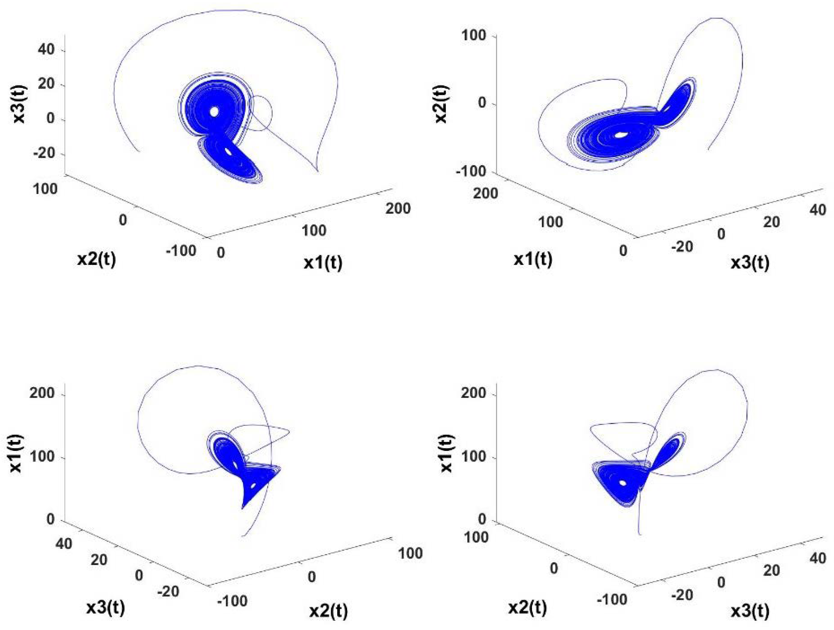
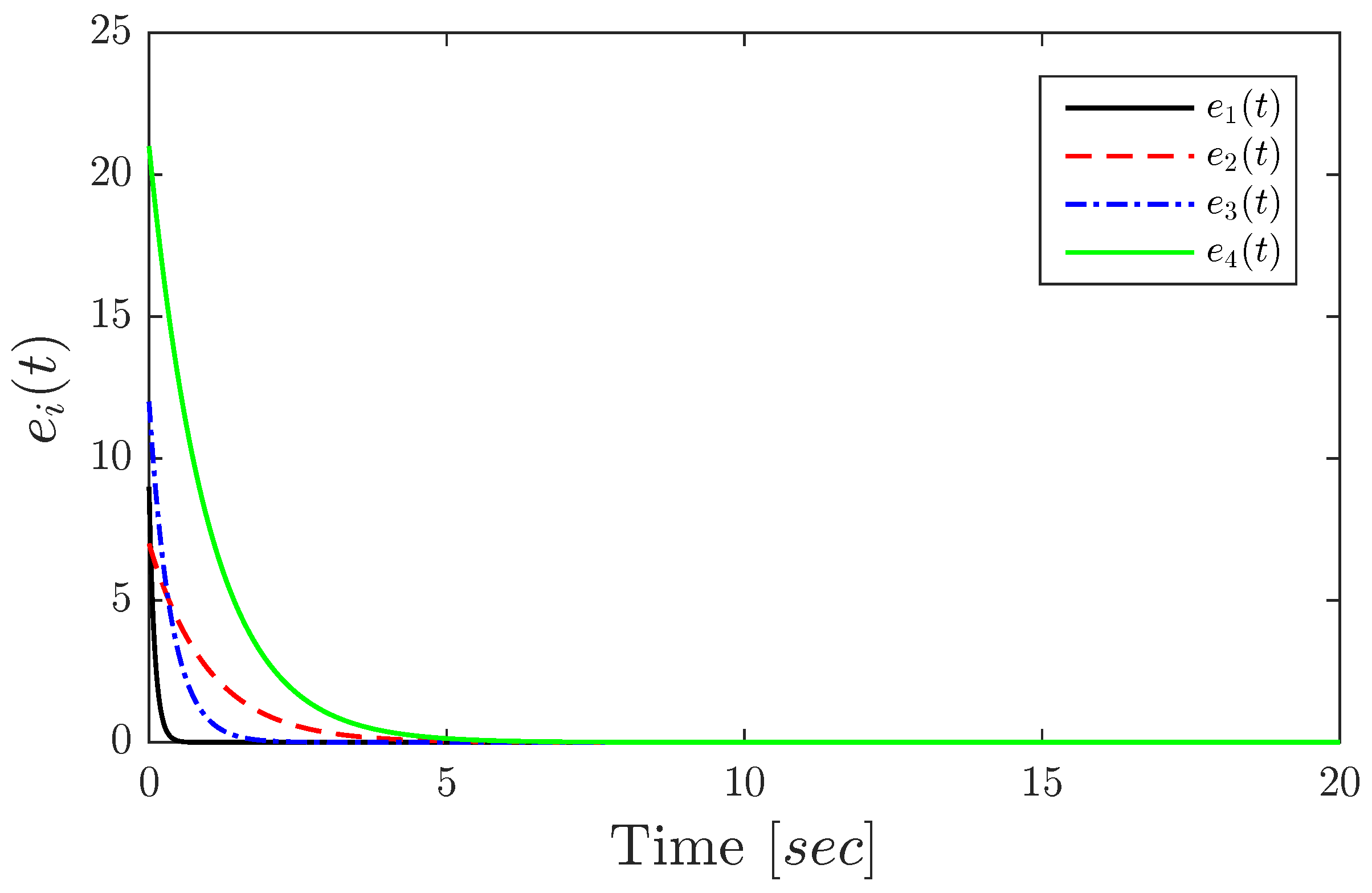
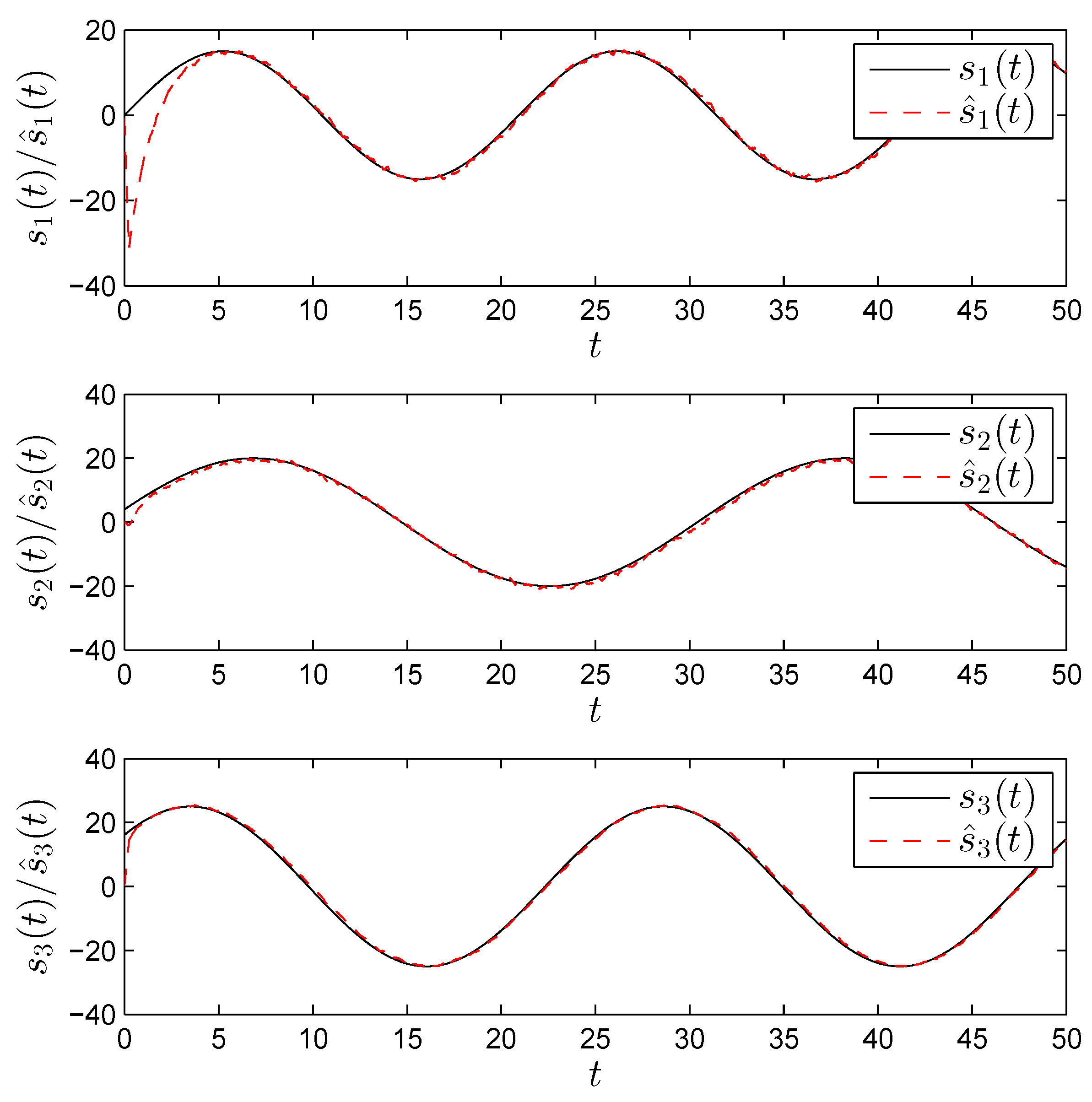
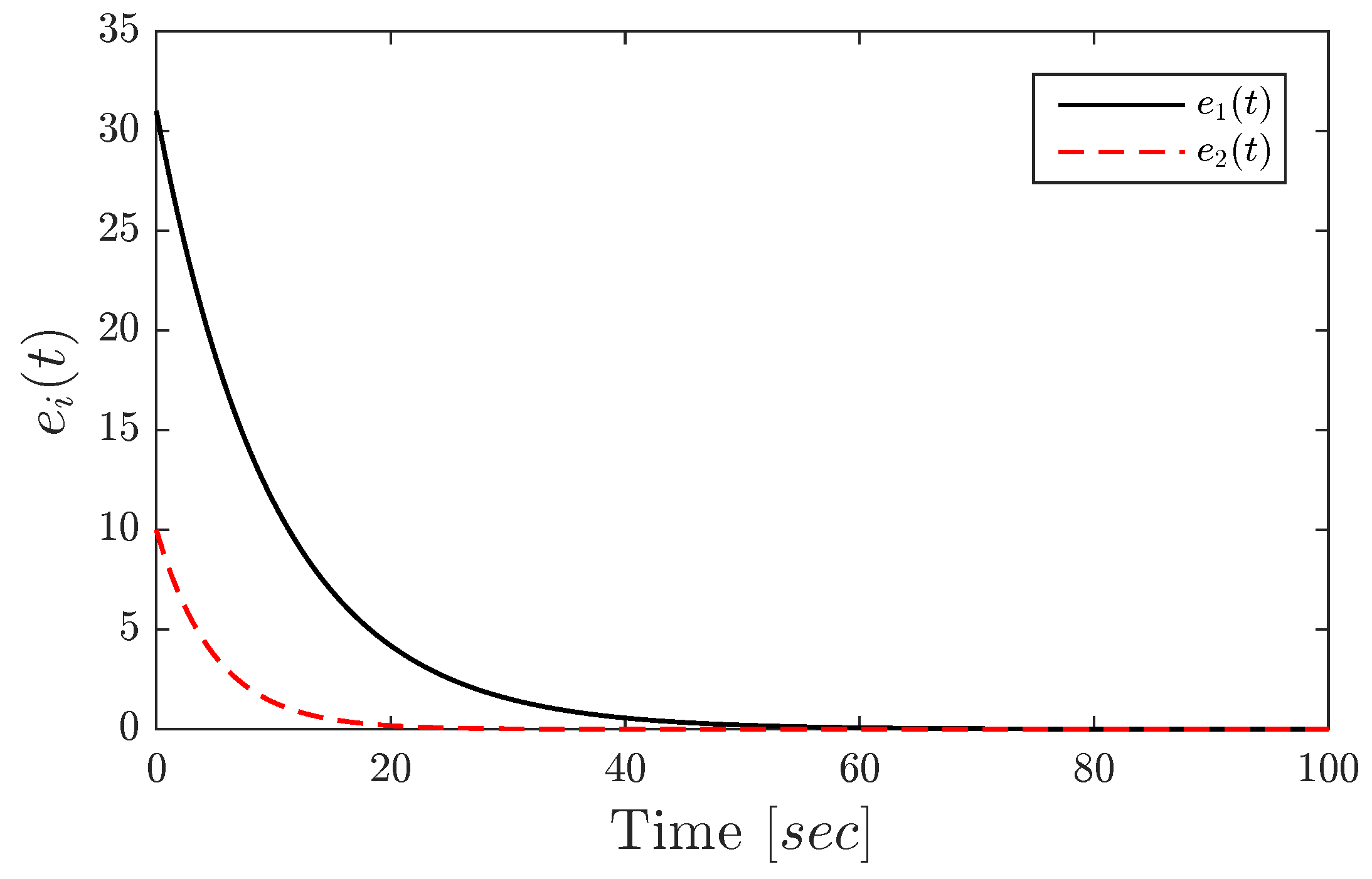
4. Numerical Example

In this section, we present some numerical simulations that verify and illustrate the effectiveness of the theoretical analysis in Section 3. It is noted that the Adams–Bashforth–Moulton method with the step size 0.001 [25,26]. We consider as master the fractional order permanent magnet synchronous motor (PMSM) model presented in [27]. A PMSM is a type of alternating current (AC) synchronous motor that uses permanent magnets to produce torque even at zero speed and can have a higher torque density compared to other types of motors. In terms of its mathematical model, it is considered a nonlinear coupling system with multiple variables. Traditionally, the PMSM was modeled as an integer-order dynamical system, which only takes into consideration the local knowledge of the states and inputs. The basic idea behind the fractional model in [27] is that, unlike integer calculus, fractional calculus involves an infinite number of terms. These terms can be employed to represent the past history of an arbitrary dynamical system. The considered model is of the form

$$D_t^{p}X\left(t\right)=f\left(X\left(t\right)\right),$$

(29)

where $X\left(t\right)={\left(x_1,x_2,x_3\right)}^T$,

$$f\left(X\left(t\right)\right)=\left(\begin{array}{c}-x_1+x_2{x}_3\\ -x_2-x_1{x}_3+a{x}_3\\ b\left(x_2-x_3\right)\end{array}\right),$$

$\left(a,b\right)=\left(100,10\right)$, and $p=0.95$.

As for the slave system, let us also consider the 4-component hyperchaotic fractional order system proposed in [28] with the addition of a control term yielding

$$D_t^{q}Y\left(t\right)=BY\left(t\right)+g\left(Y\left(t\right)\right)+U,$$

(30)

with

$$B=\left(\begin{array}{cccc}-10& 10& 0& 0\\ 28& 1& 0& -1\\ 0& 0& -\frac{8}{3}& 0\\ 0& 0& 0& 0\end{array}\right),G=\left(\begin{array}{c}0\\ -y_1{y}_3\\ -y_1{y}_2\\ 0.1y_2{y}_3\end{array}\right),\mathrm{and}U=\left(\begin{array}{c}{u}_1\\ u_2\\ u_3\\ u_4\end{array}\right).$$

The authors of [28] showed that, subject to $0.916\le q\le 1$, the system always exhibits hyperchaotic behavior. Hence, we choose the arbitrary fractional order $q=0.94$. System (30) was proposed as the fractional counterpart of the integer-order hyperchaotic system proposed in [29]. A new modified generalized projective synchronization scheme was developed for (30) and applied to a secure communication system in [28].

The chaotic attractors of the proposed master and slave systems are depicted in Figure 1 and Figure 2, respectively. The $\mathbf{F}$–$\mathbf{M}$ synchronization strategy aims to force the error

$$e\left(t\right)=\mathbf{F}\left(y_1,y_2,y_3,y_4\right)-\mathbf{M}\left(t\right)\times {\left(x_1,x_2,x_3\right)}^T$$

(31)

to zero as $t\to +\infty$. Recall from Remark 1 that our choice of matrix $\mathbf{M}$ and function $\mathbf{F}$ can lead to different types of conventional synchronization schemes. In the following, we present numerical results confirming the validity and convergence of the proposed control schemes for $d=m=4$, $d=3<m$, $d=2<m$, respectively.

Figure 1. Chaotic attractors of the master system (29) when $\left(a,b\right)=\left(100,10\right)$ and $p=0.95$.

Figure 2. Attractors of the slave system (30) when $q=0.94$ and $u_1=u_2=u_3=u_4=0$.

Case 1.

For $d=m=4$, we may choose

$$\mathbf{F}=\left(\begin{array}{c}{y}_1+y_3+y_4\\ 2y_2+y_4\\ 3y_3\\ 4y_4\end{array}\right)\mathit{and}\mathbf{M}\left(t\right)=\left(\begin{array}{ccc}\frac{1}{t+1}& 0& 1\\ 1& cost& 4\\ 1& 2& 0\\ exp\left(-t\right)& 2& 3\end{array}\right),$$

(32)

leading to

$$\mathbf{DF}\left(Y\left(t\right)\right)=\left(\begin{array}{cccc}1& 0& 1& 1\\ 0& 2& 0& 1\\ 0& 0& 3& 0\\ 0& 0& 0& 4\end{array}\right)\mathit{and}{\mathbf{D}}^{-1}=\left(\begin{array}{cccc}1& 0& 0& 0\\ 0& 2& 0& 0\\ 0& 0& 3& 0\\ 0& 0& 0& 4\end{array}\right).$$

Our choice of control matrix C must satisfy condition (13) as stated in Theorem 1. For instance, we may consider

$$C=\left(\begin{array}{cccc}0& 10& 0& 0\\ 28& 2& 0& -1\\ 0& 0& 0& 0\\ 0& 0& 0& 1\end{array}\right),$$

(33)

as all the eigenvalues of $B-C$ have negative real parts. The resulting error system may be described by

$$\left\{\begin{array}{c}{\dot{e}}_1=-10e_1,\hfill \\ {\dot{e}}_2=-e_2,\hfill \\ {\dot{e}}_3=-\frac{8}{3}{e}_3,\hfill \\ {\dot{e}}_4=-e_4.\hfill \end{array}\right.$$

Its evolution over time is depicted in Figure 3 for initial conditions ${\left(e_1\left(0\right),e_2\left(0\right),e_3\left(0\right),e_4\left(0\right)\right)}^T={\left(9,7,12,21\right)}^T$. Clearly, the error decays to zero given sufficient time, which means that the master and slave are synchronized.

Figure 3. Time evolution of the synchronization error for the 4D case.

Case 2.

For $d=3<m$, we have

$$\mathbf{F}=\left(\begin{array}{c}{y}_1+y_4^2\\ y_2+y_4\\ y_3+1\end{array}\right)\mathit{and}\mathbf{M}\left(t\right)=\left(\begin{array}{ccc}1& sint& 0\\ 2& 0& \frac{1}{1+ln\left(t+1\right)}\\ 0& \frac{1}{1+\sqrt{t}}& 3\end{array}\right),$$

(34)

yielding

$${\mathbf{D}}_1=\left(\begin{array}{cccc}1& 0& 0& 2y_4\\ 0& 2& 0& 1\\ 0& 0& 1& 0\end{array}\right),\mathit{and}{\mathbf{D}}_2=\left(\begin{array}{c}2y_4\\ 1\\ 0\end{array}\right).$$

(35)

In order to satisfy control rule (22), we must first calculate ${\mathbf{D}}_1^{-1}$, which turns out to be

$${\mathbf{D}}_1^{-1}=\left(\begin{array}{ccc}1& 0& 0\\ 0& \frac{1}{2}& 0\\ 0& 0& 1\end{array}\right).$$

(36)

The control constants ${\left(c_i\right)}_{1\le i\le 3}$ can then be chosen as

$$\left(c_1,c_2,c_3\right)=\left(1,2,3\right).$$

The error system is described by

$$\left\{\begin{array}{c}{\dot{e}}_1=-e_1,\hfill \\ {\dot{e}}_2=-2e_2,\hfill \\ {\dot{e}}_3=-3e_3.\hfill \end{array}\right.$$

Figure 4, displays the time evolution of the error with initial conditions ${\left(e_1\left(0\right),e_2\left(0\right),e_3\left(0\right)\right)}^T={\left(36,6,3\right)}^T$:

$$\left(\begin{array}{c}{e}_1\left(0\right)\\ e_2\left(0\right)\\ e_3\left(0\right)\end{array}\right)=\left(\begin{array}{c}36\\ 6\\ 3\end{array}\right).$$

(37)

Figure 4. Time evolution of the synchronization error for the 3D case.

Case 3.

As for the two-dimensional case, we consider the matrices

$$\mathbf{F}=\left(\begin{array}{c}2y_1+y_2+y_3{y}_4\\ y_1+2y_2+y_3^2+y_4^2\end{array}\right)\mathit{and}\mathbf{M}\left(t\right)=\left(\begin{array}{ccc}3& 0& cost\\ 0& 1& sint\end{array}\right),$$

(38)

which leads to

$${\mathbf{D}}_1=\left(\begin{array}{cccc}2& 1& y_4& y_3\\ 1& 2& 2y_3& 2y_4\end{array}\right),{\mathbf{D}}_2=\left(\begin{array}{cc}{y}_4& y_3\\ 2y_3& 2y_4\end{array}\right)\mathit{and}{\mathbf{D}}_1^{-1}=\left(\begin{array}{cc}1& 0\\ 0& 1\end{array}\right).$$

(39)

In this case, the control constants can be chosen as $\left(c_1,c_2\right)=\left(0.1,0.2\right)$ and yielding the error system

$$\left\{\begin{array}{c}{\dot{e}}_1=-0.1e_1,\hfill \\ {\dot{e}}_2=-0.2e_2.\hfill \end{array}\right.$$

The time-evolution of the error is depicted in Figure 5 for ${\left(e_1\left(0\right),e_2\left(0\right)\right)}^T={\left(31,10\right)}^T$.

Figure 5. Time evolution of the synchronization error for the 2D case.

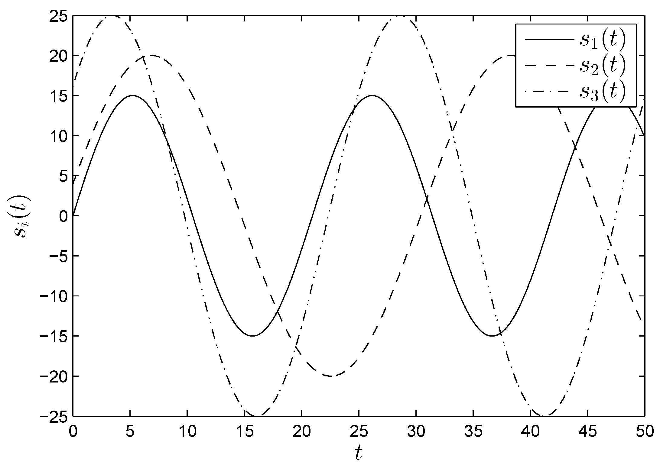
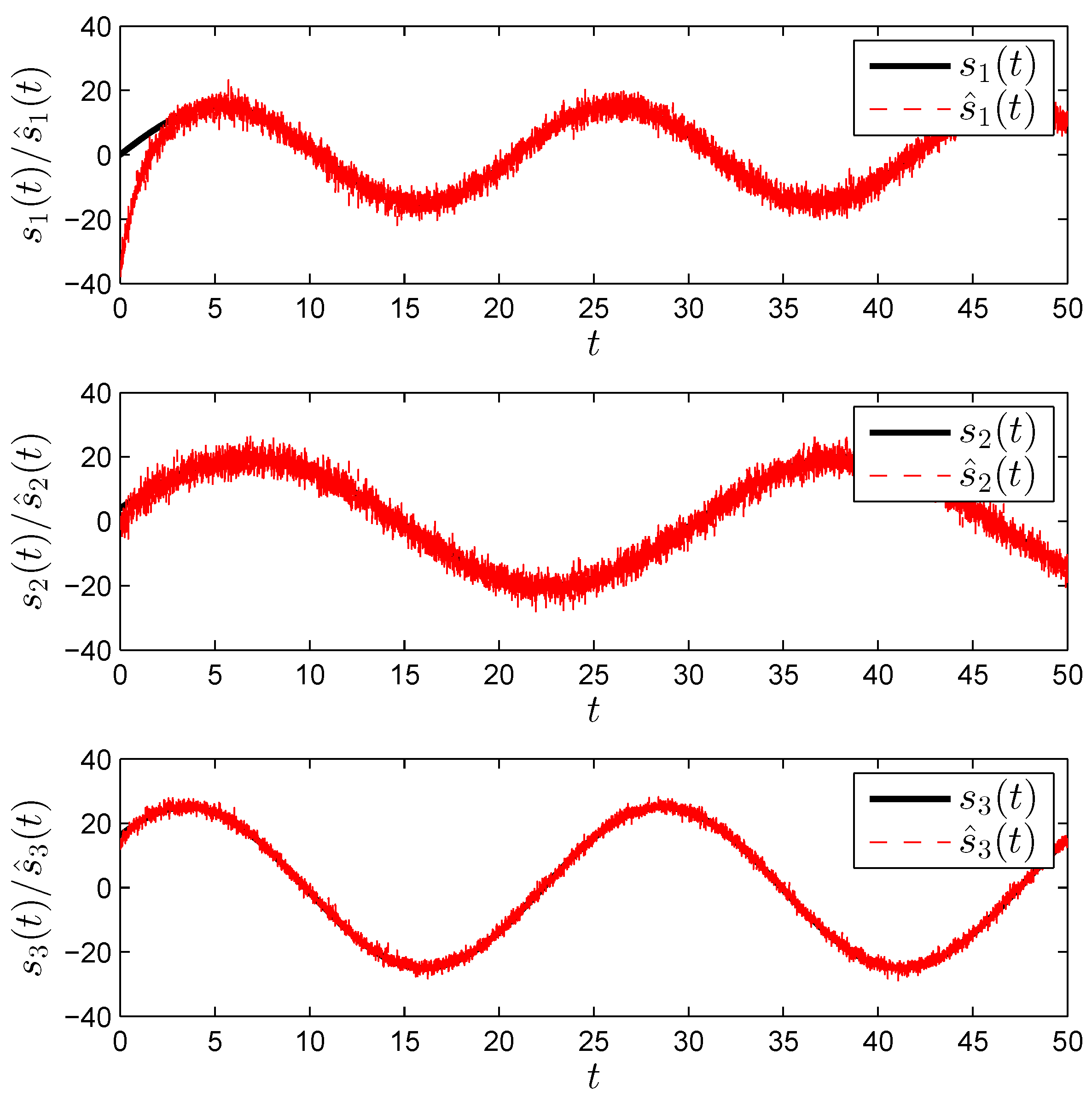
5. Application to MIMO Secure Communications

A simple communication system was developed in [28] where system (30) was used as both the master and slave. In our case, we will consider the same master–slave pair from the previous section, i.e., (29) and (30) yielding the pair

$$\left\{\begin{array}{c}{D}_t^{p}X\left(t\right)=f\left(X\left(t\right)\right),\hfill \\ D_t^{q}Y\left(t\right)=BY\left(t\right)+g\left(Y\left(t\right)\right)+U.\hfill \end{array}\right.$$

The basic idea here is to use the master–slave combination to form a multiple input multiple output (MIMO) secure communications system. MIMO uses multiple antennas at both ends of the transmission in order to send/receive multiple messages simultaneously, thereby increasing the throughput (data rate) of the system. Several MIMO communication schemes have been proposed in the literature such as [30,31], but none of these schemes have attracted much attention.

In this section, we assume an $\mathbf{F}$–$\mathbf{M}$ synchronization strategy with a dimension $d=3$. Recall from the last section that we chose

$$\mathbf{F}=\left(\begin{array}{c}{y}_1+y_4^2\\ y_2+y_4\\ y_3+1\end{array}\right)\mathrm{and}\mathbf{M}\left(t\right)=\left(\begin{array}{ccc}1& sint& 0\\ 2& 0& \frac{1}{1+ln\left(t+1\right)}\\ 0& \frac{1}{1+\sqrt{t}}& 3\end{array}\right).$$

Assuming that we want to transmit three different streams in the form $S\left(t\right)={\left(s_1\left(t\right),s_2\left(t\right),s_3\left(t\right)\right)}^T$, we can define the transmitted signals by

$$\tilde{S}\left(t\right)=\mathbf{M}\left(t\right)X\left(t\right)+S\left(t\right).$$

Note that this proposed scheme can be considered a masking algorithm as each message is hidden inside a chaotic signal. Normally, the message signals are transmitted through a common medium such as air, a copper wire, or an optical fiber. The effect of the medium on the signals is two fold. First, the signals are coupled, meaning that each antenna at the receiver is pinged by a combination of all transmitted streams. Second, consecutive symbols transmitted from the same antenna undergo a phenomenon referred to as inter-symbol interference (ISI), which is a result of the low-pass and dynamic nature of the transmission medium. For simplicity, let us assume a narrowband channel $\mathbf{H}$, whereby ISI is ignored. The received signals are given by

$$R\left(t\right)=\mathbf{H}\tilde{S}\left(t\right)+V\left(t\right),$$

with $V\left(t\right)$ being a vector of additive white Gaussian noise (AWGN) streams. At the receiver, a process known as equalization is usually used to reverse the effect of the channel. A wide variety of equalization schemes can be found in the literature, most of which require some form of training in order to estimate the channel matrix $\mathbf{H}$. These include zero-forcing, minimum mean square error (MMSE), decision feedback (DF), precoding, and many more. For the purpose of our study, we assume an MMSE equalizer of the form

$$\mathbf{W}={\left({\mathbf{H}}^H\mathbf{H}+{\sigma }^{-1}\mathbf{I}\right)}^{-1}{\mathbf{H}}^H,$$

where $\sigma$ is the signal–to–noise ratio (SNR) per stream and ${\left(·\right)}^{-1}$ denotes the inverse of a square nonsingular matrix. It is easy to see that for $\sigma =0$, this is simply the pseudo–inverse of ${\mathbf{H}}^H$, which is known as the zero–forcing equalizer. The inclusion of $\sigma$ aims to minimize the noise amplification by the equalizer. After equalization, we have

$$\begin{array}{ccc}\hfill \tilde{R}\left(t\right)& =& \mathbf{W}R\left(t\right)\hfill \\ & =& \mathbf{W}\left[\mathbf{H}\tilde{S}\left(t\right)+V\left(t\right)\right]\hfill \\ & \approx & \tilde{S}\left(t\right)+\mathbf{W}V\left(t\right)\hfill \\ & \approx & \tilde{S}\left(t\right).\hfill \end{array}$$

We now go back to the chaotic slave, which is synchronized to the master by means of a training sequence. The synchronization process is based on Theorem 2 as we saw in Case 2 of the previous section where the control parameters were chosen as $\left(c_1,c_2,c_3\right)=\left(1,2,3\right)$. Once synchronization is achieved, we end up with

$$\mathbf{F}\left(Y\left(t\right)\right)-\mathbf{M}\left(t\right)X\left(t\right)\approx \mathbf{0},$$

which allows us to reconstruct the original messages as

$$\begin{array}{ccc}\hfill \widehat{S}\left(t\right)& =& \tilde{R}\left(t\right)-\mathbf{F}\left(Y\left(t\right)\right)\hfill \\ & \approx & S\left(t\right).\hfill \end{array}$$

In order to test the theory, computer simulations were carried out on Matlab, where the source messages were assumed to be sinusoidal of the form

$$s_i\left(t\right)=A_{i}sin\left({\omega }_{i}t+{\phi }_i\right),i=1,2,3,$$

with

$$\begin{array}{ccc}{A}_1=15,\hfill & {\omega }_1=0.3,\hfill & {\phi }_1=0,\hfill \\ A_2=20,\hfill & {\omega }_2=0.2,\hfill & {\phi }_2=0.5,\hfill \\ A_3=25,\hfill & {\omega }_3=0.25,\hfill & {\phi }_3=0.7.\hfill \end{array}$$

Note that ${\omega }_i$ denotes the normalized angular frequency. The resulting sine waves are depicted in Figure 6. Figure 7 shows the transmitted and equalized signals, respectively. After synchronization is achieved, the two waveforms overlap. The random-like chaotic nature of the transmitted signals is apparent. Figure 8 shows the recovered messages. Clearly, the recovered messages contain additive noise, which is a natural consequence of the amplifications employed at the receiver as well as imperfections in the equalization process. A low–pass filter can be used to combat the noise as can be seen in Figure 9.

Figure 6. The original messages $s_i\left(t\right)$ to be transmitted by n transmit antennas in a MIMO secure communication system.

Figure 7. The transmitted signals ${\tilde{s}}_i\left(t\right)$ as well as the equalized signals ${\tilde{r}}_i\left(t\right)$ for an SNR of 40 dB.

Figure 8. The recovered messages ${\widehat{s}}_i\left(t\right)$ from the n receive antennas.

Figure 9. The recovered messages ${\widehat{s}}_i\left(t\right)$ from the n receive antennas after a 50–tap low–pass filter.

6. Conclusions

This paper investigated the $\mathbf{F}$–$\mathbf{M}$ synchronization with index d of fractional-order systems differential systems with non–identical dimensions. The main novelty of this piece of work is the combination of two distinct types of synchronization, namely generalized synchronization based on a functional relationship $\mathbf{F}$ and inverse matrix projective synchronization based on a matrix $\mathbf{M}$. The developed approach exploits nonlinear controllers and the stability theory of integer-order systems in order to synchronize an m-dimensional slave with an n-dimensional master system. The approach has proved to be effective in achieving synchronized dynamics not only when the synchronization index d is equal to the slave’s dimension m, but even when $d<m$. To the best of the authors’ knowledge, this finding is both novel and forms a considerable contribution to the field of study.

In order to confirm the findings of this study and highlight the capabilities of the developed scheme, a numerical example was considered where the master is a 3D chaotic fractional system and the slave is a 4D hyperchaotic fractional system. In addition, a MIMO communications system employing $\mathbf{F}$–$\mathbf{M}$ synchronization was proposed and verified through computer simulations. In the proposed system, matrix $\mathbf{M}$ is used to condition the master chaotic states used to mask our messages and function $\mathbf{F}$ is used to condition the slave states. When synchronization is achieved, the two become identical and the masked messages are recovered.

References