An Ensemble Classifier with Random Projection for Predicting Protein–Protein Interactions Using Sequence and Evolutionary Information

Abstract

Identifying protein–protein interactions (PPIs) is crucial to comprehend various biological processes in cells. Although high-throughput techniques generate many PPI data for various species, they are only a petty minority of the entire PPI network. Furthermore, these approaches are costly and time-consuming and have a high error rate. Therefore, it is necessary to design computational methods for efficiently detecting PPIs. In this study, a random projection ensemble classifier (RPEC) was explored to identify novel PPIs using evolutionary information contained in protein amino acid sequences. The evolutionary information was obtained from a position-specific scoring matrix (PSSM) generated from PSI-BLAST. A novel feature fusion scheme was then developed by combining discrete cosine transform (DCT), fast Fourier transform (FFT), and singular value decomposition (SVD). Finally, via the random projection ensemble classifier, the performance of the presented approach was evaluated on Yeast, Human, and H. pylori PPI datasets using 5-fold cross-validation. Our approach achieved high prediction accuracies of 95.64%, 96.59%, and 87.62%, respectively, effectively outperforming other existing methods. Generally speaking, our approach is quite promising and supplies a practical and effective method for predicting novel PPIs.

1. Introduction

Proteins are fundamental to human life and seldom function as a single unit. They always interact with each other in a specific way to perform cellular processes [1]. As a consequence, the analysis of protein–protein interactions (PPIs) can help researchers reveal tissue functions and structures and identify the pathogenesis of human diseases and drug targets of gene therapy. Recently, various high-throughput experimental techniques have been discovered for PPI detection, including a yeast two-hybrid system [2], immunoprecipitation [3], and protein chips [4]. However, the biological experiments are generally costly and time-consuming. Moreover, both false negative and false positive rates of these methods are very high [2,5]. Therefore, the development of reliable calculating models for the prediction of PPIs has great practical significance.

To construct a computational method for PPI prediction, the most important factor is to extract highly discriminative features that can effectively describe proteins. So far, protein feature extraction methods are based on many data types, such as genomic information [6,7], structure information [8,9], evolutionary information [10,11], and amino acid sequence information. Of these approaches, sequence-based methods are more readily available, and it has demonstrated that protein amino acid sequence information is important for detecting PPIs [12,13,14,15,16]. Martin et al. used a descriptor called a “signature product” to discover PPIs [12]. The signature product is a product of sub-sequences from a protein sequence and extends the signature descriptor from chemical information. Shen et al. presented a conjoint triad (CT) approach to take the characters of amino acids and their adjacent amino acids into account [13]. Guo et al. proposed an auto covariance (AC) descriptor approach to represent an amino acid sequence with a foundation of seven different physicochemical scales [14]. When they detected Yeast PPIs, prospective prediction accuracy was achieved. Wong et al. employed the physicochemical property response matrix combined with the local phase quantization descriptor (PR-LPQ) to extract the eigen value of the proteins [15]. Considering the evolutionary information of protein, Huang et al. adopted substitution matrix representation (SMR) based on BLOSUM62 to construct a feature vector and achieved promising prediction accuracy [16]. Ding et al. proposed a novel protein sequence representation method based on a matrix to predict PPIs via an ensemble classification method [17]. Wang et al. proposed a computational method based on a probabilistic classification vector machine (PCVM) model and a Zernike moment (ZM) descriptor to identify PPIs from amino acids sequences [18]. Lei et al. employed the NABCAM (the neighbor affinity-based core-attachment method) to identify protein complexes from dynamic PPI networks [19]. Nanni et al. summarized and evaluated a couple of feature extraction methods for describing protein amino acids sequences by verifying them on multiple datasets, and they constructed an ensemble of classifiers for sequence-based protein classification, which not only performed well on many datasets but was also, under certain conditions, superior to the state of the art [20,21,22,23].

Next, the computational methods for PPI prediction can be formulated as a binary classification problem. A number of machine learning-based computational models for PPI prediction have emerged. Ronald et al. proposed a technique of applying Bayesian networks to detect PPIs on the Yeast dataset [24]. Qi et al. employed several classifiers, including support vector machine (SVM), decision tree (DT), random forest (RF), and logistic regression (LR), to compare their performances in predicting PPIs [25].

Of machine-learning-based computational models for PPI prediction, one of the most important challenges is that the high-dimensional features may include unimportant information and noise, leading to the over-fitting of classification systems [26,27]. Previous works have shown that random projection (RP) is a high-efficiency and sufficient precision approach that can reduce the dimensions of many high-dimensional datasets [28,29,30]. However, the performance using a single RP method is poor [31] because of the instability of RP. Therefore, in our study, an RP ensemble method was designed to predict PPIs.

The capacity of the integration model was better and more effective than that of separate runs of the RP approach. Moreover, the ensemble algorithm achieved results that are also superior to those of similar schemes that use principal component analysis (PCA) to reduce the dimensionality of the dataset [32]. The RP-ensemble-based classifier has useful features [33]. Firstly, RP maintains the geometrical structure of the dataset with a certain distortion rate when its dimensionality is reduced. This feature can reduce the complicacy of the classifier and the difficulty of new sample classification. In addition, dimensionality reduction can eliminate redundant information and reduce generalization error. Particularly, instead of relying on a single classifier, the RP ensemble method incorporates several classifiers that are superior to each single classifier. This feature can lead to better and more stable classification results.

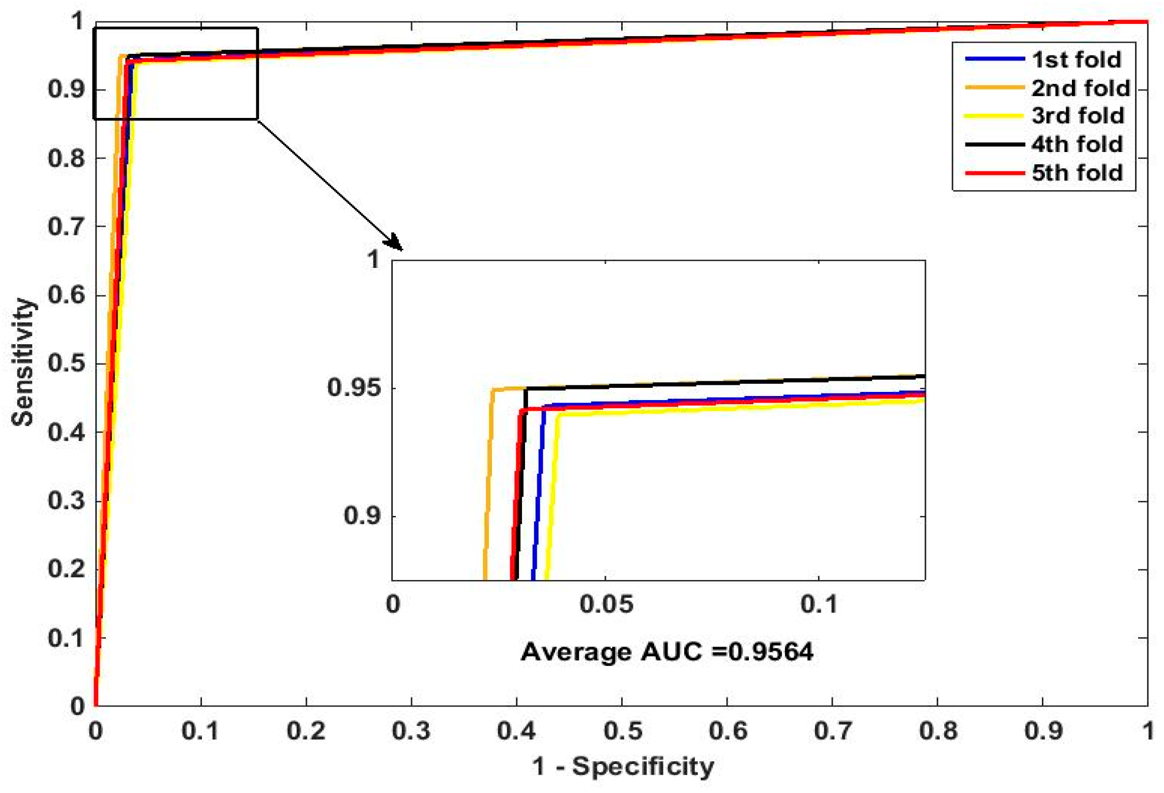
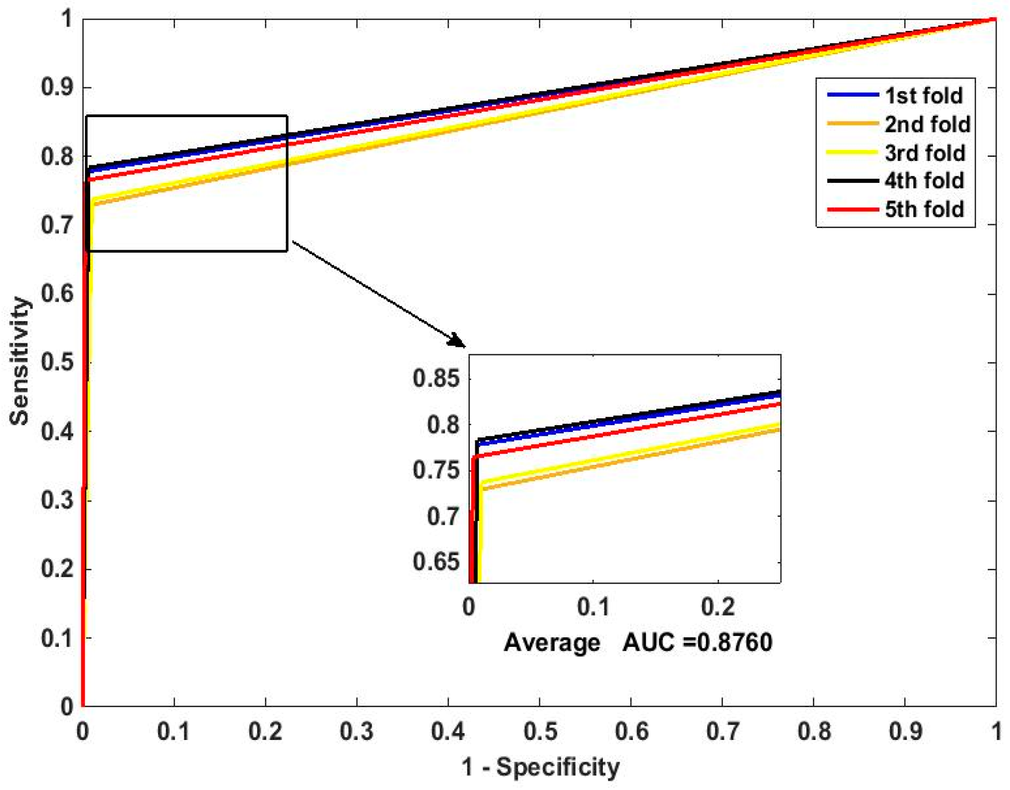
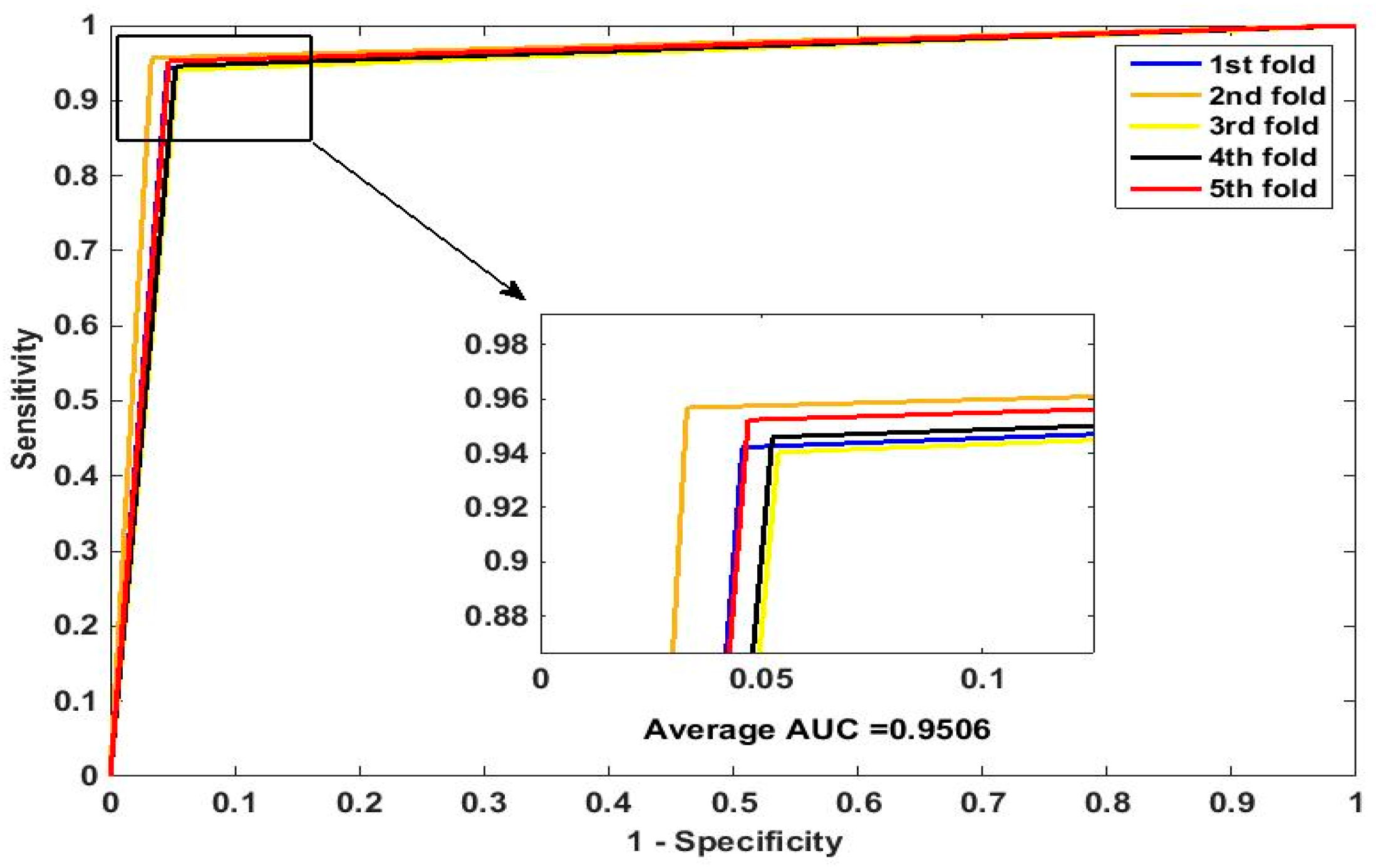
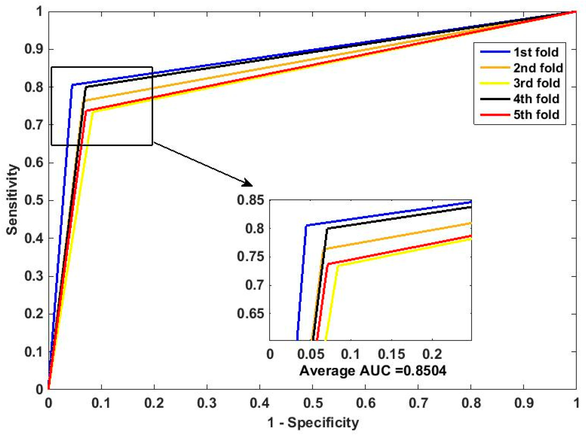
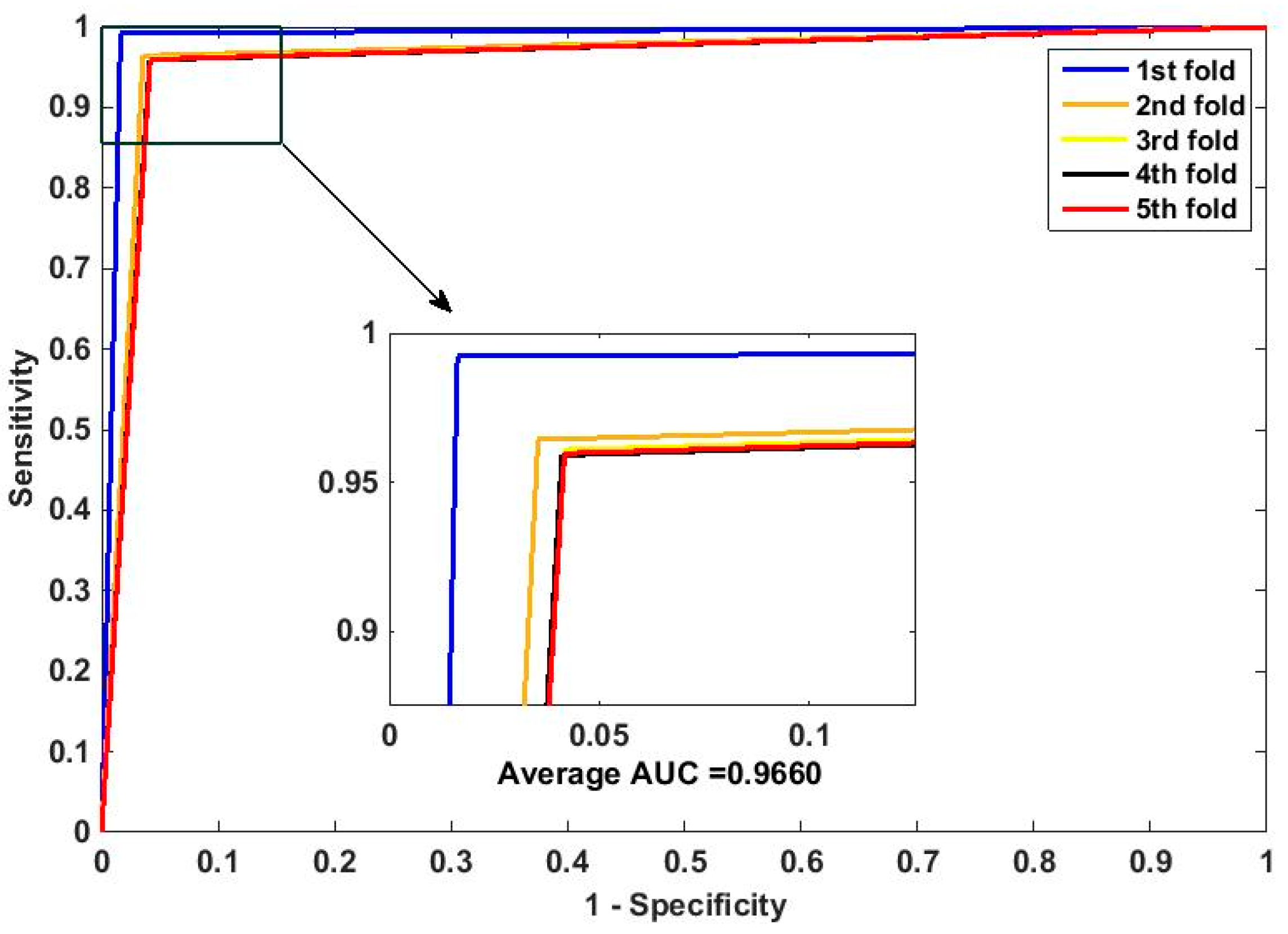
In this paper, we propose an RPEC-based approach for detecting PPIs by combining a protein sequence with its evolutionary information. Firstly, a position-specific scoring matrix (PSSM) is used to express the amino acid sequence. Secondly, three 400 dimensional feature vectors are extracted from the PSSM matrix by using DCT, FFT, and SVD, respectively, and each protein sequence is described as a 2400 size of eigen vector. Then, an 1000 dimensionally reduced feature vector is obtained via PCA. Finally, the RP ensemble model is built by employing the feature matrix of the protein pairs as an input to predict PPIs. Our method is estimated on the PPI datasets of Yeast, Human, and H. pylori and yields higher prediction accuracy of 95.64%, 96.59% and 87.62%, respectively. When compared with the SVM classifier fed into the same feature vector, the accuracies of our method are increased by 0.58%, 1.4%, and 2.57%, respectively. We also compare our method with other approaches. The obtained outcomes prove that our method is much better at predicting PPIs than those of previous works.

2. Materials and Methods

2.1. Position-Specific Scoring Matrix

A position-specific scoring matrix (PSSM) can be applied to search distantly related proteins. It emerged from a group of sequences formerly arranged by structural or similarity [34]. There are many methods of calculating distances and metric spaces [35,36]. Here, some research on PSSM methods and its relation to amino acids is discussed. Liu et al. [37] discovered that the PSSM profile has been shown to provide a useful source of information for improving the prediction performance of the protein structural class. Wang et al. [38] proposes two fusion feature representations of DipPSSM and PseAAPSSM to integrate PSSM with DipC and PseAAC, respectively. In our method, we predict PPIs based on PSSM. Thus, each protein can be converted to a PSSM by using the Position-Specific Iterated Basic Local Alignment Search Tool (PSI-BLAST) [39].

The PSSM can be described as follows:

$$PSSM=(N_1,N_2,\cdots ,N_i,\cdots ,N_{20})$$

(1)

where $N_m={(N_{1m},N_{2m},\cdots ,N_{Lm})}^T,(m=1,2,\cdots ,20)$. With a size of $L\times 20$ PSSM, L represents the length of an amino acid, and 20 is the number of amino acids. In our research, we achieved the experiment datasets by using PSI-BLAST to use a PSSM for PPI detection. In order to achieve a wide and analogous sequences, the parameter e-value of PSI-BLAST was adjusted to 0.001 and opted for three iterations, and the other values in PSI-BLAST were defaults. Finally, the PSSM from a certain protein sequence was expressed as a $M\times 20$ matrix, where M denotes the quantity of residues, and 20 indicates the number of amino acids.

2.2. Discrete Cosine Transform

Discrete cosine transform (DCT) is a classical orthogonal transformation, which was first proposed in the 1970s by Ahmed [40]. It is used in image compression processing with lossy signals because of its strong compaction performance. DCT has better energy aggregation than others. It can convert spatial signals into frequency domains and thus work well in de-correlation. DCT can be defined as follows:

$$\mathrm{DCT}\left(i,j\right)=k_i{k}_j{\displaystyle \sum _{m=0}^{M-1}{\displaystyle \sum _{n=0}^{N-1}Sig\left(m,n\right)}\cos \frac{\pi \left(2m+1\right)i}{2M}\cdot \cos }\frac{\pi \left(2n+1\right)i}{2N},\begin{array}{cc}& 0\le i\le M,0\le j\le N\end{array}$$

(2)

where

$$k_i=\{\begin{array}{l}\frac{1}{\sqrt{M}},i=0\\ \sqrt{\frac{2}{M}},1\le i\le M-1\end{array}\begin{array}{ccc},& & k_j=\{\begin{array}{l}\frac{1}{\sqrt{N}},i=0\\ \sqrt{\frac{2}{N}},1\le i\le M-1\end{array}\end{array}$$

(3)

The N × 20 PSSM is the input signal, which is x_i ∈ Rⁿ. Here, we can obtain 400 coefficients as the protein feature vector after the DCT feature descriptor. At the end, we can obtain a feature vector whose dimension is 800 from each protein pair via DCT.

2.3. Fast Fourier Transform

Fast Fourier transform (FFT) is a feature extraction method. The simplified energy function for FFT algorithms evaluate in the space of protein partner mutual orientations. The mesh displacements of one protein centroid in regard to another protein centroid can represent the translational space [41].

Here we describe the simplified energy scoring function, as PPIs are defined on a mesh and indicate M correlation functions all possible values of l, m, and n (assuming that one protein is the ligand and the other is the receptor):

$$f(l,m,n)={\displaystyle \sum _M{\displaystyle \sum _{a,b,c}Rp}}(a,b,c)Lp(a+l,b+m,c+n)$$

(4)

where Lp(a,b,c) and Rp(a,b,c) are the integral part of the related function defined with protein interactions on the ligand and the receptor, respectively. We can thus use M forward and an inverse fast Fourier transform to calculate the expression efficiently, and the forward and inverse fast Fourier transform can be denoted by FT and IFT, respectively:

$$f(l,m,n)=IFT\left\{{\displaystyle \sum _M^{p}FT*\left\{Rp\right\}FT\left\{Lp\right\}}\right\}(l,m,n)$$

(5)

$$FT\{H\}(i,j,k)={\displaystyle \sum _{i,j,k}H(a,b,c){\exp }^{-2\pi a(ia/N_1+jb/N_2+kc/N_3)}}$$

(6)

$$IFT\{h\}(a,b,c)=\frac{1}{N_1{N}_2{N}_3}{\displaystyle \sum _{i,j,k}h(i,j,k)}{\exp }^{-2\pi a(ia/N_1+jb/N_2+kc/N_3)}$$

(7)

where $a=\sqrt{-1}, N_1, N_2$ and N₃ are grid sizes of the three coordinates. If $N_1=N_2=N_3=N$, the complexity of this method is O(N³ log(N³)). Then, we can use FFT to compute the related function of Lp with the pre-calculated function of Rp. The final sum offers the scoring values of function for all probable conversions of the ligands. Finally, we obtained and sorted the results from different rotations.

2.4. Singular Value Decomposition

It is a challenge for bioinformatics to explore effective methods for analyzing global gene expression data. Singular value decomposition (SVD) is a common technique for multivariate data analysis [42]. We assumed that M is the size of an m × n matrix. The decomposition for SVD can be expressed as follows:

$$M=US{V}^{\ast }$$

(8)

where U means an m × m unitary matrix, S indicates a positive semi-definite m × n diagonal matrix, V represents an n × n unitary matrix, and V* is a conjugate transposed of V. As a result, we can obtain the singular value of the matrix with proteins. The columns of U form the base vector of orthogonal input or analysis for M and are called left singular vectors. Rows of V* form the base vector of orthogonal output for M and are called right singular vectors. Thus, the diagonal element values of S are singular.

2.5. Principal Component Analysis

Principal component analysis (PCA) is a data-dimensionally reduced method. PCA is widely used for data analysis, and the variable interacting with information from the dimensionally reduced dataset can persist [43,44]. It embeds samples in high-dimensional space into low-dimensional space, and the dimensionally reduced data represents the original data as closely as possible. The PCA of a data matrix determines the main information from a matrix according to a complementary group of scores and loading diagrams.

Furthermore, PCA converts primitive variables into a linear combination set, the principal components (PCs), which catch the data variables, are linearly independent, and are weighted in decreasing order of variance coverage [45]. This can reduce the data dimension directly by discarding low variability characteristic elements. In this way, all original α-dimensional datasets can be optimally implanted in a feature space with lower dimension.

The concept and calculation of PCA technology is simple. It can be expressed as follows: Given $\mathrm{M}=A_{ij}(i=1,2,\cdots ,\alpha ;j=1,2,\cdots ,\beta )$, where A_ij denotes the feature value of the j-th sample with the i-th feature. Firstly, α-dimensional means that the full datasets with vector μ_j and α × α covariance matrix are calculated. Secondly, the feature vectors and feature values are calculated and sorted according to decreasing feature values. These feature vectors can be expressed as F₁ with feature value λ₁, as F₂ with feature value λ₂, and so on. The largest k feature vectors can then be obtained. This can be done by observing the frequency content of feature vectors. The maximum feature values are equivalent to the dimensions which is the large variance of the dataset. Finally, we can construct an α × k matrix X, whose rows denote the number of samples, and k makes up the feature vectors. Afterwards, the lower dimensional feature space’s number of k (k < α) was transformed by N = X^TM(A). It is thus shown that the representation can minimize the square error criterion.

2.6. Random Projection Ensemble Classifier

Machine learning has been extensively applied in many fields. In mathematical statistics, RP is a method for reducing the dimensionality of a series of points that lie in Euclidean space. Compared with other methods, the RP method is simpler and has less output error. It has been successfully used in the reconstruction of dispersion signals, facial recognition, and textual and visual information retrieval. Now we introduce the RP algorithm in detail.

Let $\mathrm{\Gamma }={\left\{x_i\right\}}_{i=1}^N$ be a series of column vectors in primitive data space with high dimension. $x_i\in R^n$, n is the high dimension, and N denotes the number of columns. Dimensionality reduction embeds the vectors into a space R^q, which has lower dimension than Rⁿ, where q << n. The output results are column vectors in the space with lower dimension.

$$\tilde{\mathrm{\Gamma }}={\left\{\widetilde{x_i}\right\}}_{i=1}^N\widetilde{x_i}\in R^q$$

(9)

where q is close to the intrinsic dimensionality of $\mathrm{\Gamma }$ [46,47]. The embedded vectors refer to the vectors in the set $\mathrm{\Gamma }$.

Here, if we want to employ the RP model to reduce the dimensionality of $\mathrm{\Gamma }$, a random vector set $\gamma ={\left\{r_i\right\}}_{i=1}^n$ must be structured first, where $r_i\in R^q$. There are two choices in structuring the random basis:

(1)

The vectors ${\left\{r_i\right\}}_{i=1}^n$ are spread on the $q$-dimensional unit spherical surface.

(2)

The components of ${\left\{r_i\right\}}_{i=1}^n$ conform to Bernoulli +1/+2 distribution and the vectors are standardized such that ${\Vert r_i\Vert }_{l_2}=1$ for $i=1,\cdots ,n$.

We generated a $q\times n$ matrix R, where q consists of the vectors in $\gamma$. n was mentioned in the previous paragraph. The projecting result $\widetilde{x_i}$ can be obtained by

$$\widetilde{x_i}=R\cdot x_i.$$

(10)

In our method, RP is used to construct a training set on which the classifiers will be trained. The use of RP lays the foundation for our ensemble model.

Now, we illustrate the theory of our ensemble method. A training set $\mathrm{\Gamma }$ is given in Equation (9). We generate a G whose degree is $n\times N$, and G comes from the column vectors in $\mathrm{\Gamma }$.

$$G=\left(x_1|x_2\cdots |x_N\right).$$

(11)

We then structure ${\left\{R_i\right\}}_{i=1}^k$, whose size is $q\times n$, where $q$ and $n$ are introduced in the preceding paragraph, k means the size of ensemble classifiers. The columns are standardized so as to the $l_2$ norm is 1.

In the ensemble classifiers, we constructed the training sets ${\left\{T_i\right\}}_{i=1}^k$ by means of projecting G onto ${\left\{R_i\right\}}_{i=1}^k$.

$$T_i=R_i\cdot G\begin{array}{cc}& i=1,\cdots ,k\end{array}.$$

(12)

They are then fed into the base classifier, and the outcomes are a group of classifiers ${\left\{{\ell }_i\right\}}_{i=1}^k$. For the sake of classifying a fresh set $u$ with classifier ${\ell }_i$, firstly, $u$ will be inlaid into the target space $R^q$. It can be obtained by embedding $u$ into $R_i$.

$$\tilde{u}=R_i\cdot u$$

(13)

where $\tilde{u}$ is the result of embedding. The classification of $\tilde{u}$ can be garnered by ${\ell }_i$. In this ensemble algorithm, the RP ensemble classifier will use the classification result of all classifiers ${\left\{{\ell }_i\right\}}_{i=1}^k$ of $\tilde{u}$ to decide the final result with a majority voting scheme.

In this study, the 1000 coefficients were divided into 100 non-overlapping blocks. We chose the projection from a block of size 10 that obtained the smallest test error with the leave-one-out test error estimate. We used the k-Nearest Neighbor (KNN) as a base classifier, where k = seq(1, 25, by = 3). Prior probability of interaction pairs in the calculated training samples dataset was considered as the voting parameter.

3. Results

3.1. Datasets Construction

We collected the highly reliable Saccharomyces cerevisiae PPI dataset from the DIP database of DIP_20071007 (http://dip.doe-mbi.ucla.edu) [48]. Protein sequences less than 50 residues may be fragments. Thus, we directly removed these protein pairs. In addition, much of the sequence identity of protein pairs is usually deemed as homologous. To eliminate the effects of these homologous sequence pairs, those with ≥40% sequence identity from protein pairs were also deleted. Finally, we used the remaining 5594 protein pairs as a positive PPI dataset and constructed a negative dataset with 5594 other pairs from distinct subcellular localizations. The final Yeast PPI dataset in our experiment was composed of 11,188 protein pairs with 50% positive samples and 50% negative samples.

For the sake of evaluating the universality of our model, we also performed the proposed method on Human and Helicobacter pylori datasets. The Human dataset was gathered from the Human Protein Reference database (HPRD). We also removed protein pairs with ≥25% sequence identity. To construct a golden standard positive dataset, we chose the remaining 3899 interacting protein pairs among 2502 different Human proteins. Because the proteins in diverse subcellular fractions cannot interact with each other, we built a golden standard negative dataset by selecting 4262 protein pairs among 661 distinct Human proteins [49]. Finally, the Human dataset was composed of 8161 protein pairs. Another PPI dataset used in this study was made of 2916 Helicobacter pylori protein pairs, which are mentioned by Martin et al. [12]. In this dataset, there are 1458 interacting pairs and 1458 non-interacting pairs.

3.2. Evaluation Measurements

In order to assess the capability of the RP classifier, the accuracy (Acc), sensitivity (Sen), precision (PE), and Mathews’ correlation coefficient (MCC) were used as evaluation indexes. They can be described as follows:

$$Acc=\frac{TP+TN}{TP+FP+TN+FN}$$

(14)

$$Sen=\frac{TP}{TP+FN}$$

(15)

$$PE=\frac{TP}{TP+FP}$$

(16)

$$MCC=\frac{TP\times TN-FP\times FN}{\sqrt{\left(TP+FN\right)\times \left(TN+FP\right)\times \left(TP+FP\right)\times \left(TN+FN\right)}}$$

(17)

where true positive (TP) indicates the count of true samples predicted to interact; false negative (FN) is the quantity of interacting samples predicted to not interact; false positive (FP) is the count of non-interacting samples predicted to interact; true negative (TN) is the number of true samples predicted to not interact.

3.3. Experimental Environment

In the study, the presented sequence-based PPI prediction system was carried out using MATLAB (R2014a, the Math Works, Inc., Natick, MA, USA) and R programming language (X64 3.3.1, Copyright© 2016 The R Foundation for Statistical Computing). We finished the experiment with a machine with a 2.4 GHz 2-core CPU and an 8 GB memory based on operating system of Windows. We adapted an RP ensemble classifier to predict PPIs and applied an RP ensemble classifier to train the datasets in the experiment, and the k-Nearest Neighbor (KNN) was employed as a base classifier, where k = seq(1, 25, by = 3).

3.4. Performance of PPI Prediction

Three different PPI datasets were applied to estimate the results of our presented model. They are Yeast, Human and H. pylori PPI datasets, respectively.

3.4.1. Performance of the Proposed Method with Three Diverse PPI Datasets

In our problem of PPI predictions, the dimension of input features is 2400, which may contain the unimportant information and noise. Thus, the PCA algorithm is used to eliminate noise in the dataset. However, it is hard to determine the optimal number of features to use. Here, we carried out the experiments to find the optimal PCA dimension. For the sake of example, for the H. pylori PPI dataset, the prediction performance of different PCA dimensions is shown in

Table 1. The prediction performance of different principal component analysis (PCA) dimensions on the H. pylori protein–protein interaction (PPI) dataset.

Dimension	600-D (%)	700-D (%)	800-D (%)	900-D (%)	1000-D (%)	1100-D (%)	1200-D (%)	1300-D (%)	1400-D (%)
Accuracy	81.82	68.78	78.90	68.27	88.51	84.91	79.25	71.36	85.59
Sensitivity	63.67	80.95	84.42	62.04	77.82	71.10	60.98	80.07	72.05
Specificity	98.36	58.06	73.94	73.79	99.31	99.65	96.96	62.06	99.65
Precision	97.25	62.96	74.44	67.73	99.13	99.53	95.11	69.25	99.53
MCC	66.86	39.78	58.44	36.12	78.90	73.27	62.32	42.91	74.30

. As a result, the favorable number of PCA dimensions is 1000-dimensional.

For the sake of avoiding over-fitting and of verifying the constancy of the model, 5-fold cross-validations were used, which is part of the sub-sampling test method. More specifically, in 5-fold cross-validation, the entire dataset is split into 5 parts, where 4 parts are applied as training samples and 1 part is used as testing samples. In this way, we obtain five models from the datasets, and each model is a separate experiment. The prediction results of three datasets with the RP ensemble classifier are based on protein sequences and evolutionary information shown in

Table 2. Result of random projection (RP) classifier on the Yeast PPI dataset using 5-fold cross-validation.

Testing Set	Acc (%)	PE (%)	Sen (%)	MCC (%)
Yeast1	95.35	96.51	94.31	90.73
2	96.33	97.46	94.95	92.69
3	94.99	96.28	93.96	90.01
4	95.93	96.65	94.97	91.87
5	95.58	96.85	94.15	91.19
Average	95.64 ± 0.52	96.75 ± 0.45	94.47 ± 0.47	91.30 ± 1.03

,

Table 3. Result of RP classifier on Human PPI dataset using 5-fold cross-validation.

Testing Set	Acc (%)	PE (%)	Sen (%)	MCC (%)
Human1	98.77	98.20	99.22	97.55
2	96.45	96.19	96.43	92.88
3	95.96	95.34	96.09	91.89
4	95.89	95.54	95.90	91.78
5	95.90	95.61	95.97	91.79
Average	96.59 ± 1.24	96.18 ± 1.17	96.72 ± 1.41	93.18 ± 2.49

and

Table 4. Result of RP classifier on H. pylori PPI dataset using 5-fold cross-validation.

Testing Set	Acc (%)	PE (%)	Sen (%)	MCC (%)
H. pylori1	88.51	99.13	77.82	78.90
2	86.79	99.51	72.76	75.86
3	86.11	98.65	73.74	74.83
4	88.51	99.16	78.33	78.99
5	88.18	99.55	76.47	78.41
Average	87.62 ± 1.10	99.20 ± 0.36	75.82 ± 2.47	77.40 ± 1.92

.

As shown in Table 2, Table 3 and Table 4, when predicting the Yeast PPI dataset by applying our proposed method, we gained the average Acc, PE, Sen, and MCC of 95.64%, 96.75%, 94.47% and 91.30%, respectively. The standard deviations of Acc, PE, Sen, and MCC are 0.52%, 0.45%, 0.47% and 1.03%, respectively. When predicting the Human PPI dataset, good results are obtained: the average Acc, PE, Sen, and MCC are 96.59%, 96.18%, 96.72%, and 93.18%, respectively. The standard deviations are 1.24%, 1.17%, 1.41% and 2.49%, respectively. When predicting the H. pylori PPI dataset, the average Acc, PE, Sen, and MCC are 87.62%, 99.20%, 75.82% and 77.40%, with the corresponding standard deviations of 1.10%, 0.36%, 2.47% and 1.92%, respectively.

The Receiver Operating Characteristic (ROC) curves for Yeast, Human, and H. pylori PPI datasets with five-fold cross-validation are shown in Figure 1, Figure 2 and Figure 3, respectively. We computed the average AUC (area under ROC curve) values of Yeast, Human, and H. pylori PPI datasets to be 0.9570, 0.9615, and 0.8287, respectively. In conclusion, the higher accuracies and lower standard deviations of these values indicate that our presented approach is feasible and reasonable for detecting PPIs.

Compared with the Human and the Yeast PPI datasets, the prediction performance of the H. pylori dataset is lower. It should be noticed that the sample sizes of the Human, Yeast, and H. pylori datasets are 8161, 11,188, and 2916, respectively. We found that the prediction performance, as indicated by the accuracy score, improves as the size of the samples increases.

3.4.2. Performance Comparison between the RP Classifier and the SVM Model

Many machine learning techniques and algorithms are employed to predict PPIs. We compared our RP model with the state-of-the-art SVM model. During the experiment, we extracted the feature values by the same method to ensure fairness. We used the LIBSVM toolbox on http://www.csie.ntu.edu.tw/~cjlin/libsvm/. The radial basis function (RBF) kernel was applied in our experiments. The method of a gridding search was employed to optimize two kernel parameters: C and g.

For the Yeast PPI dataset, we use the optimized parameters C = 0.3 and g = 1. The obtained results as shown in

Table 5. The proposed method and the SVM-based method tested on the three datasets with 5-fold cross-validation. The numbers which are bold means the largest values of performance.

Dataset	Classifier	Acc (%)	PE (%)	Sen (%)	MCC (%)
Yeast	PSSM + RPEC	95.64 ± 0.52	96.75 ± 0.45	94.47 ± 0.47	91.30 ± 1.03
	PSSM + SVM	95.06 ± 0.72	95.35 ± 0.74	94.76 ± 0.69	90.60 ± 1.31
Human	PSSM + RPEC	96.59 ± 1.24	96.18 ± 1.17	96.72 ± 1.41	93.18 ± 2.49
	PSSM + SVM	95.19 ± 1.30	94.91 ± 1.45	95.04 ± 1.53	90.84 ± 2.38
H. pylori	PSSM + RPEC	87.62 ± 1.10	99.20 ± 0.36	75.82 ± 2.47	77.40 ± 1.92
	PSSM + SVM	85.05 ± 2.26	91.92 ± 1.79	76.80 ± 3.38	74.27 ± 3.30

. For Human and H. pylori PPI datasets, the optimized penalty parameters are 0.06 and 0.5, and the kernel function parameters are 2 and 0.3, respectively.

When we predicted the PPIs by applying the SVM classifier on the Yeast dataset, we obtained an average Acc, PE, Sen, and MCC of 95.06%, 95.35%, 94.76% and 90.60%, respectively. Compared with the SVM classifier, the accuracy of our method is higher by about 0.58%. When we predicted the Human PPI dataset, the results based on the SVM classifier of the average accuracy, precision, sensitivity, MCC, respectively, were 95.19%, 94.91%, 95.04% and 90.84%, respectively. Compared with the SVM classifier, the accuracy of our method was higher by about 1.40%. On the H. pylori dataset, the SVM classifier achieved an 85.05% average accuracy and a 91.92% precision, with 76.80% sensitivity and 74.27% MCC. Compared with the SVM classifier, the accuracy of our method was higher by about 2.57%.

Based on data in Table 5, the average accuracy, precision, and sensitivity values of our proposed model are much higher than averages attained by the SVM approach. The higher the standard deviation, the more unstable the algorithm is. Furthermore, we plotted the ROC curves on the three datasets by applying the SVM classifier as shown in Figure 4, Figure 5 and Figure 6. It can be seen that the AUC areas yielded by our method are higher than those of the SVM classifier.

3.4.3. Comparison with Other Methods

There have been many prediction approaches developed for detecting PPIs. To further estimate the capacity of the proposed model, we compared our method with other existing methods.

Table 6. Different methods tested on the Yeast PPI dataset using 5-fold cross-validation. The numbers which are bold means the largest values of performance.

Method	Feature	Classifier	Acc (%)	PE (%)	Sen (%)	MCC (%)
You’s work [50]	MLD	RF	94.72 ± 0.43	98.91 ± 0.33	94.34 ± 0.49	85.99 ± 0.89
You’s work [45]	Multiple	E-ELM	87.00 ± 0.29	87.59 ± 0.32	86.15 ± 0.43	77.36 ± 0.44
You’s work [51]	MCD	SVM	91.36 ± 0.36	91.94 ± 0.62	90.67 ± 0.69	84.21 ± 0.59
Wong’s work [15]	PR-LPQ	RoF	93.92 ±0.36	96.45 ± 0.45	91.10 ± 0.31	88.56 ± 0.63
Guo’s work [14]	ACC	SVM	89.33 ± 2.67	88.87 ± 6.16	89.93 ± 3.68	N/A
Guo’s work [14]	AC	SVM	87.36 ± 1.38	87.82 ± 4.33	87.30 ± 4.68	N/A
Zhou’s work [52]	LD	SVM	88.56 ± 0.33	89.50 ± 0.60	87.37 ± 0.22	77.15 ± 0.68
Yang’s work [53]	LD	KNN	86.15 ± 1.17	90.24 ± 1.34	81.03 ± 1.74	N/A
Our Method	PSSM	RPEC	95.64 ± 0.52	96.75 ± 0.45	94.47 ± 0.47	91.30 ± 1.03

shows the results of diverse approaches to the Yeast PPI dataset. The accuracies obtained by other previous methods range from 86.15% to 94.72%. In contrast, our method achieves an average accuracy of 95.64%. Our method obtained a higher PE and Sen than that of eight other methods. In conclusion, compared with all methods from Table 6, our method obtained the highest Acc and MCC in the Yeast PPI dataset.

Similarly, we compared our method with five other existing methods on the Human dataset. Based on

Table 7. Different methods tested on the Human PPI dataset using 5-fold cross-validation. The numbers which are bold means the largest values of performance.

Model	Acc (%)	PE (%)	Sen (%)	MCC (%)
LDA + RoF	95.70	N/A	97.6	91.8
LDA + SVM	90.70	N/A	89.7	81.3
AC + RF	95.50	N/A	94	91.4
AC + RoF	95.10	N/A	93.3	91
AC + SVM	89.30	N/A	94	79.2
Our Method	96.59 ± 1.24	96.18 ± 1.17	96.72 ± 1.41	93.18 ± 2.49

, which shows the results of diverse approaches on the Yeast PPI dataset, the accuracies obtained by other previous methods range from 89.30% to 95.70%. In contrast, our method achieves an average accuracy of 96.59%. Accordingly, our method outperforms better than most other approaches, which are also based on ensemble classifiers.

4. Discussion and Conclusions

In the post-genome era, it is quite important to predict PPIs using computational techniques. In the study, we proposed a PPI prediction model by extracting evolutionary information from the position-specific scoring matrix (PSSM) generated by PSI-BLAST. Then, an RP ensemble classifier is used to implement PPI prediction. We conducted experiments on Yeast, Human, and H. pylori PPI datasets. In order to evaluate the capacity of our model, we compared our approach with an SVM-based model as well as other existing methods. The results of our model are quite promising; our model is a beneficial supplement to traditional experimental methods for PPI prediction. Moreover, the RPEC method may also be employed to solve other classification problems.

References

1. Gavin, A.-C.; Bösche, M.; Krause, R.; Grandi, P.; Marzioch, M.; Bauer, A.; Schultz, J.; Rick, J.M.; Michon, A.-M.; Cruciat, C.-M. Functional organization of the yeast proteome by systematic analysis of protein complexes. Nature 2002, 415, 141–147. [Google Scholar] [CrossRef] [PubMed]
2. Ito, T.; Chiba, T.; Ozawa, R.; Yoshida, M.; Hattori, M.; Sakaki, Y. A comprehensive two-hybrid analysis to explore the yeast protein interactome. Proc. Natl. Acad. Sci. USA 2001, 98, 4569–4574. [Google Scholar] [CrossRef] [PubMed]
3. Williams, N.E. Immunoprecipitation procedures. Methods Cell Biol. 1999, 62, 449–453. [Google Scholar]
4. Zhu, H.; Bilgin, M.; Bangham, R.; Hall, D.; Casamayor, A.; Bertone, P.; Lan, N.; Jansen, R.; Bidlingmaier, S.; Houfek, T. Global analysis of protein activities using proteome chips. Science 2001, 293, 2101–2105. [Google Scholar] [CrossRef] [PubMed]
5. Uetz, P.; Giot, L.; Cagney, G.; Mansfield, T.A.; Judson, R.S.; Knight, J.R.; Lockshon, D.; Narayan, V.; Srinivasan, M.; Pochart, P. A comprehensive analysis of protein-protein interactions in saccharomyces cerevisiae. Nature 2000, 403, 623–627. [Google Scholar] [CrossRef] [PubMed]
6. Osbourn, A.E.; Field, B. Operons. Cell. Mol. Life Sci. 2009, 66, 3755–3775. [Google Scholar] [CrossRef] [PubMed]
7. Marcotte, C.J.V.; Marcotte, E.M. Predicting functional linkages from gene fusions with confidence. Appl. Bioinform. 2002, 1, 93–100. [Google Scholar]
8. Hue, M.; Riffle, M.; Vert, J.-P.; Noble, W.S. Large-scale prediction of protein-protein interactions from structures. BMC Bioinform. 2010, 11, 144. [Google Scholar] [CrossRef] [PubMed] [Green Version]
9. Aloy, P.; Querol, E.; Aviles, F.X.; Sternberg, M.J. Automated structure-based prediction of functional sites in proteins: Applications to assessing the validity of inheriting protein function from homology in genome annotation and to protein docking. J. Mol. Biol. 2001, 311, 395–408. [Google Scholar] [CrossRef] [PubMed]
10. Swapna, L.S.; Srinivasan, N.; Robertson, D.L.; Lovell, S.C. The origins of the evolutionary signal used to predict protein-protein interactions. BMC Evol. Biol. 2012, 12, 238. [Google Scholar] [CrossRef] [PubMed]
11. Burger, L.; Van Nimwegen, E. Accurate prediction of protein-protein interactions from sequence alignments using a bayesian method. Mol. Syst. Biol. 2008, 4, 165. [Google Scholar] [CrossRef] [PubMed]
12. Martin, S.; Roe, D.; Faulon, J.-L. Predicting protein-protein interactions using signature products. Bioinformatics 2004, 21, 218–226. [Google Scholar] [CrossRef] [PubMed]
13. Shen, J.; Zhang, J.; Luo, X.; Zhu, W.; Yu, K.; Chen, K.; Li, Y.; Jiang, H. Predicting protein-protein interactions based only on sequences information. Proc. Natl. Acad. Sci. USA 2007, 104, 4337–4341. [Google Scholar] [CrossRef] [PubMed]
14. Guo, Y.; Yu, L.; Wen, Z.; Li, M. Using support vector machine combined with auto covariance to predict protein-protein interactions from protein sequences. Nucleic Acids Res. 2008, 36, 3025–3030. [Google Scholar] [CrossRef] [PubMed]
15. Wong, L.; You, Z.-H.; Li, S.; Huang, Y.-A.; Liu, G. Detection of Protein-Protein Interactions from Amino Acid Sequences Using a Rotation Forest Model with a Novel pr-lpq Descriptor; Springer: Cham, Switzerland, 2015; pp. 713–720. [Google Scholar]
16. Huang, Y.A.; You, Z.H.; Gao, X.; Wong, L.; Wang, L. Using weighted sparse representation model combined with discrete cosine transformation to predict protein-protein interactions from protein sequence. BioMed Res. Int. 2015, 2015, 902198. [Google Scholar] [CrossRef] [PubMed]
17. Ding, Y.; Tang, J.; Guo, F. Identification of protein-protein interactions via a novel matrix-based sequence representation model with amino acid contact information. Int. J. Mol. Sci. 2016, 17, 1623. [Google Scholar] [CrossRef] [PubMed]
18. Wang, Y.; You, Z.; Li, X.; Chen, X.; Jiang, T.; Zhang, J. Pcvmzm: Using the probabilistic classification vector machines model combined with a zernike moments descriptor to predict protein-protein interactions from protein sequences. Int. J. Mol. Sci. 2017, 18, 1029. [Google Scholar] [CrossRef] [PubMed]
19. Lei, X.; Liang, J. Neighbor affinity-based core-attachment method to detect protein complexes in dynamic ppi networks. Molecules 2017, 22, 1223. [Google Scholar] [CrossRef]
20. Nanni, L.; Brahnam, S.; Lumini, A. High performance set of pseaac and sequence based descriptors for protein classification. J. Theor. Biol. 2010, 266, 1–10. [Google Scholar] [CrossRef] [PubMed]
21. Nanni, L.; Lumini, A.; Brahnam, S. An empirical study of different approaches for protein classification. Sci. World J. 2014, 2014. [Google Scholar] [CrossRef] [PubMed]
22. Nanni, L.; Lumini, A. An ensemble of k-local hyperplanes for predicting protein-protein interactions. Bioinformatics 2006, 22, 1207–1210. [Google Scholar] [CrossRef] [PubMed]
23. Nanni, L.; Lumini, A.; Gupta, D.; Garg, A. Identifying bacterial virulent proteins by fusing a set of classifiers based on variants of chou’s pseudo amino acid composition and on evolutionary information. IEEE/ACM Trans. Comput. Biol. Bioinform. 2012, 9, 467–475. [Google Scholar] [CrossRef] [PubMed]
24. Jansen, R.; Yu, H.; Greenbaum, D.; Kluger, Y.; Krogan, N.J.; Chung, S.; Emili, A.; Snyder, M.; Greenblatt, J.F.; Gerstein, M. A bayesian networks approach for predicting protein-protein interactions from genomic data. Science 2003, 302, 449–453. [Google Scholar] [CrossRef] [PubMed]
25. Qi, Y.; Bar-Joseph, Z.; Klein-Seetharaman, J. Evaluation of different biological data and computational classification methods for use in protein interaction prediction. Proteins Struct. Funct. Bioinform. 2006, 63, 490–500. [Google Scholar] [CrossRef] [PubMed]
26. Wang, Y.-B.; You, Z.-H.; Li, X.; Jiang, T.-H.; Chen, X.; Zhou, X.; Wang, L. Predicting protein-protein interactions from protein sequences by a stacked sparse autoencoder deep neural network. Mol. BioSyst. 2017, 13, 1336–1344. [Google Scholar] [CrossRef] [PubMed]
27. Wang, Y.-B.; You, Z.-H.; Li, L.-P.; Huang, Y.-A.; Yi, H.-C. Detection of interactions between proteins by using legendre moments descriptor to extract discriminatory information embedded in pssm. Molecules 2017, 22, 1366. [Google Scholar] [CrossRef] [PubMed]
28. Bourgain, J. On lipschitz embedding of finite metric spaces in hilbert space. Isr. J. Math. 1985, 52, 46–52. [Google Scholar] [CrossRef]
29. Emmanuel, C.; Romberg, J.; Tao, T. Robust uncertainty principles: Exact signal reconstruction from highly incomplete frequency information. IEEE Trans. Inf. Theory 2004, 52, 489–509. [Google Scholar]
30. Donoho, D.L. Compressed sensing. IEEE Trans. Inf. Theory 2006, 52, 1289–1306. [Google Scholar] [CrossRef]
31. Fern, X.Z.; Brodley, C.E. Random Projection for High Dimensional Data Clustering: A Cluster Ensemble Approach. In Proceedings of the 20th International Conference on Machine Learning (ICML-03), Washington, DC, USA, 21–24 August 2003; pp. 186–193. [Google Scholar]
32. Wan, S.; Mak, M.-W.; Zhang, B.; Wang, Y.; Kung, S.-Y. Ensemble random projection for multi-label classification with application to protein subcellular localization. In Proceedings of the 2014 IEEE International Conference on Acoustics, Speech and Signal Processing (ICASSP), Florence, Italy, 4–9 May 2014; pp. 5999–6003. [Google Scholar]
33. Schclar, A.; Rokach, L. Random projection ensemble classifiers. Enterp. Inf. Syst. 2009, 24, 309–316. [Google Scholar]
34. Gribskov, M.; McLachlan, A.D.; Eisenberg, D. Profile analysis: Detection of distantly related proteins. Proc. Natl. Acad. Sci. USA 1987, 84, 4355–4358. [Google Scholar] [CrossRef] [PubMed]
35. Nieto, J.J.; Torres, A.; Georgiou, D.; Karakasidis, T. Fuzzy polynucleotide spaces and metrics. Bull. Math. Biol. 2006, 68, 703–725. [Google Scholar] [CrossRef] [PubMed]
36. Georgiou, D.; Karakasidis, T.; Nieto, J.J.; Torres, A. A study of entropy/clarity of genetic sequences using metric spaces and fuzzy sets. J. Theor. Biol. 2010, 267, 95–105. [Google Scholar] [CrossRef] [PubMed]
37. Liu, T.; Qin, Y.; Wang, Y.; Wang, C. Prediction of protein structural class based on gapped-dipeptides and a recursive feature selection approach. Int. J. Mol. Sci. 2016, 17, 15. [Google Scholar] [CrossRef] [PubMed]
38. Wang, S.; Liu, S. Protein sub-nuclear localization based on effective fusion representations and dimension reduction algorithm lda. Int. J. Mol. Sci. 2015, 16, 30343–30361. [Google Scholar] [CrossRef] [PubMed]
39. Altschul, S.F.; Madden, T.L.; Schäffer, A.A.; Zhang, J.; Zhang, Z.; Miller, W.; Lipman, D.J. Gapped blast and psi-blast: A new generation of protein database search programs. Nucleic Acids Res. 1997, 25, 3389–3402. [Google Scholar] [CrossRef] [PubMed]
40. Ahmed, N.; Natarajan, T.; Rao, K.R. Discrete cosine transform. IEEE Trans. Comput. 1974, 100, 90–93. [Google Scholar] [CrossRef]
41. Kozakov, D.; Brenke, R.; Comeau, S.R.; Vajda, S. Piper: An fft-based protein docking program with pairwise potentials. Proteins Struct. Funct. Bioinform. 2006, 65, 392–406. [Google Scholar] [CrossRef] [PubMed]
42. Wall, M.E.; Rechtsteiner, A.; Rocha, L.M. Singular value decomposition and principal component analysis. In A Practical Approach to Microarray Data Analysis; Springer: Berlin, Germany, 2003; pp. 91–109. [Google Scholar]
43. You, Z.; Wang, S.; Gui, J.; Zhang, S. A novel hybrid method of gene selection and its application on tumor classification. In Proceedings of the International Conference on Intelligent Computing: Advanced Intelligent Computing Theories and Applications—With Aspects of Artificial Intelligence, ICIC 2008, Shanghai, China, 15–18 September 2008; pp. 1055–1068. [Google Scholar]
44. Zhang, S.; Ye, F.; Yuan, X. Using principal component analysis and support vector machine to predict protein structural class for low-similarity sequences via pssm. J. Biomol. Struct. Dyn. 2012, 29, 1138–1146. [Google Scholar] [CrossRef] [PubMed]
45. You, Z.-H.; Lei, Y.-K.; Zhu, L.; Xia, J.; Wang, B. Prediction of protein-protein interactions from amino acid sequences with ensemble extreme learning machines and principal component analysis. BMC Bioinform. 2013, 14, S10. [Google Scholar] [CrossRef] [PubMed]
46. Hein, M.; Audibert, J.-Y. Intrinsic dimensionality estimation of submanifolds in r d. In Proceedings of the 22nd international conference on Machine learning, Bonn, Germany, 7–11 August 2005; pp. 289–296. [Google Scholar]
47. Hegde, C.; Wakin, M.; Baraniuk, R. Random projections for manifold learning. In Advances in Neural Information Processing Systems; Curran Associates Inc.: Vancouver, BC, Canada, 2007; pp. 641–648. [Google Scholar]
48. Salwinski, L.; Miller, C.S.; Smith, A.J.; Pettit, F.K.; Bowie, J.U.; Eisenberg, D. The database of interacting proteins: 2004 update. Nucleic Acids Res. 2004, 32, D449–D451. [Google Scholar] [CrossRef] [PubMed]
49. You, Z.-H.; Yu, J.-Z.; Zhu, L.; Li, S.; Wen, Z.-K. A mapreduce based parallel svm for large-scale predicting protein-protein interactions. Neurocomputing 2014, 145, 37–43. [Google Scholar] [CrossRef]
50. You, Z.-H.; Chan, K.C.; Hu, P. Predicting protein-protein interactions from primary protein sequences using a novel multi-scale local feature representation scheme and the random forest. PLoS ONE 2015, 10, e0125811. [Google Scholar] [CrossRef] [PubMed]
51. You, Z.-H.; Zhu, L.; Zheng, C.-H.; Yu, H.-J.; Deng, S.-P.; Ji, Z. Prediction of protein-protein interactions from amino acid sequences using a novel multi-scale continuous and discontinuous feature set. BMC Bioinform. 2014, 15, S9. [Google Scholar] [CrossRef] [PubMed]
52. Zhou, Y.Z.; Gao, Y.; Zheng, Y.Y. Prediction of protein-protein interactions using local description of amino acid sequence. Adv. Comput. Sci. Educ. Appl. 2011, 202, 254–262. [Google Scholar]
53. Zheng, X.; Wu, L.; Ye, S.; Chen, R. Simplified swarm optimization-based function module detection in protein-protein interaction networks. Appl. Sci. 2017, 7, 412. [Google Scholar] [CrossRef]
Figure 1. Receiver Operating Characteristic (ROC) curves of our method performed on the Yeast dataset. The curve provides Sensitivity (TP Rate) against 1-Specificity (FP Rate).
Applsci 08 00089 g001
Figure 2. ROC curves of our method on the Human dataset. The curve provides Sensitivity (TP Rate) against 1-Specificity (FP Rate).
Applsci 08 00089 g002
Figure 3. ROC curves of our method on the H. Pylori dataset. The curve provides Sensitivity (TP Rate) against 1-Specificity (FP Rate).
Applsci 08 00089 g003
Figure 4. ROC curves of the SVM method on the Yeast dataset. The curve provides Sensitivity (TP Rate) against 1-Specificity (FP Rate).
Applsci 08 00089 g004
Figure 5. ROC curves of the SVM method on the Human dataset. The curve provides Sensitivity (TP Rate) against 1-Specificity (FP Rate).
Applsci 08 00089 g005
Figure 6. ROC curves of the SVM method on the H. Pylori dataset. The curve provides TP Rate (Sensitivity) against 1-Specificity (FP Rate).
Applsci 08 00089 g006