CoSimulating Communication Networks and Electrical System for Performance Evaluation in Smart Grid


1
Kukka Inc., Seoul 06245, Korea
2
Network Technology R&D Center, SK Telecom, Seongnam-si, Gyeonggi-do 13595, Korea
3
School of Electrical Engineering, Korea University, Seoul 02841, Korea
4
TmaxSoft Inc., Seongnam-si, Gyeonggi-do 13613, Korea
*
Author to whom correspondence should be addressed.
Appl. Sci. 2018, 8(1), 85; https://doi.org/10.3390/app8010085
Submission received: 14 November 2017
/
Revised: 27 December 2017
/
Accepted: 5 January 2018
/
Published: 9 January 2018
Abstract
:In smart grid research domain, simulation study is the first choice, since the analytic complexity is too high and constructing a testbed is very expensive. However, since communication infrastructure and the power grid are tightly coupled with each other in the smart grid, a well-defined combination of simulation tools for the systems is required for the simulation study. Therefore, in this paper, we propose a cosimulation work called OOCoSim, which consists of OPNET (network simulation tool) and OpenDSS (power system simulation tool). By employing the simulation tool, an organic and dynamic cosimulation can be realized since both simulators operate on the same computing platform and provide external interfaces through which the simulation can be managed dynamically. In this paper, we provide OOCoSim design principles including a synchronization scheme and detailed descriptions of its implementation. To present the effectiveness of OOCoSim, we define a smart grid application model and conduct a simulation study to see the impact of the defined application and the underlying network system on the distribution system. The simulation results show that the proposed OOCoSim can successfully simulate the integrated scenario of the power and network systems and produce the accurate effects of the networked control in the smart grid.
1. Introduction
The smart grid is a new kind of electrical grid where the power system and the IT system are tightly coupled with each other. In the smart grid, various elements of the power system are managed by remote controls, which are performed based on situational awareness [1]. Moreover, the deployment of eco-friendly elements such as renewable energy generators (solar generators and wind generators) and PHEV (Plug-in Hybrid Electric Vehicle) requires a lot of information exchange and processing. The information exchange and processing can contribute to not only providing numerous electricity services, but also making power grid more stable, efficient and eco-friendly. Therefore, it is exceedingly important to investigate how we should apply the advanced computing and networking technologies to the power system in the smart grid.
There are many studies aimed to enhance the performance of the smart grid, especially the networking system. Bae et al. [2] addressed the data communication scheme for Advanced Metering Infrastructure (AMI) considering the reduction of network delay and the privacy of the smart grid users. Son et al. [3] proposed a novel voucher scheme for the secure trading between the customers of the smart grid. Furthermore, Kim et al. [4] designed a wireless communication framework which considered the signal interference of electromagnetic wave and delay-constraint of the smart grid system. Since the smart grid indicates the convergence of the network system and power distribution system, which were distinctive before, studies must be elaborately designed and clearly evaluated.
The majority of the smart grid studies usually depend on sophisticated simulation tools [5], since it is very difficult to find out a well-defined theoretical model which can represent the complexity and dynamics of the smart grid. If we try to represent the smart grid system with a mathematical model, we need to use unrealistic assumptions and/or leave out subtle details of the system. Especially, the degree of analytic complexity becomes more intractable in the distribution and customer domain [6], since many applications, such as demand-response (DR), energy management, and smart metering, operate on the domains. The applications generally collect diverse data, perform information processing, and control power system elements through the network system. Therefore, the complexity of the analytic approach rapidly increases as the number of applications and information exchanges increase. Another approach of the smart grid research is testbed based verification where numerous applications can be implemented and studies can be performed elaborately. However, the cost to construct the testbed is too expensive, since new kinds of equipments and systems should be employed. Moreover, since the smart grid is a very large system and many elements are tightly coupled, it is very difficult to construct a well specified and designed smart grid testbed.
Therefore, a simulation study is the first choice for investigating both structures and operations of the smart grid. However, since the network system and the power system are tightly coupled with each other in the smart grid, organic combination of simulation tools for both systems is required to carry out an elaborate simulation study. In this paper, the word organic is used to describe a cosimulation in which two simulators are necessary, fit together harmoniously as fundamental parts of a whole, and interact with each other systematically, so that any complex applications can be precisely modeled. However, there are several challenges to achieve the goal. One of the challenges is that the smart grid is an application-centric system [7]. Various applications would be introduced in the smart grid and each application would have different operations. Therefore, we are strongly convinced to build a cosimulation technique through which diverse applications can be easily modeled and simulated. Another challenge is that the smart grid is a mixture of large and complex systems. Therefore, we cannot build a precise cosimulation tool by extending an individual simulation tool for a single system. For example, if we employ a single network simulator which has an extension for the power system, the large scale of the power system might be simplified, so unrealistic assumptions would be introduced. Therefore, integrating independent simulators of each system would be a favorable choice for simulating smart grid.
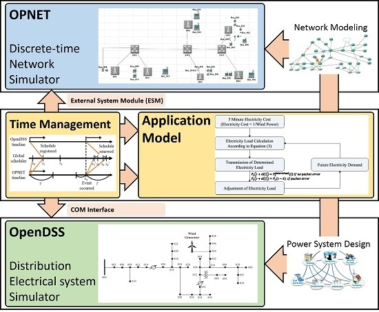
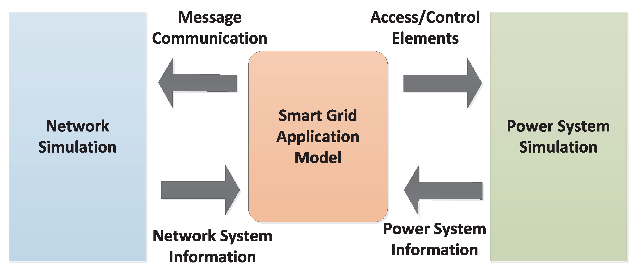
Figure 1 shows the conceptual representation of the proposed cosimulation. The application model defines the control policies, algorithms, and functions, which receive current states of the power system and event signal, and then decide the next states. The transmission of the event signals and control messages can be simulated through the network simulation. As the network simulation is invoked, the network-side information is retrieved by the application model in the context of the cosimulation. Similarly, control policies are applied to the power system simulation, and the new states information are reported to the application model. Moreover, meaningful results of the smart grid application are generated by the power system simulation, which can verify the impact of the application.
Based on the conceptual representation of the cosimulation, we propose a novel cosimulation work for the smart grid applications, called OOCoSim, which stands for OPNET [8] and OpenDSS [9] cosimulation. Since both OPNET and OpenDSS have large scalability, various applications in the future smart grid can be implemented and simulated in OOCoSim. Moreover, both OPNET and OpenDSS can operate simultaneously on the same platform (Windows platform), dynamic and organic simulation can be achieved. In the future smart grid, complex applications which require dedicated interaction, such as deciding the amount of adjustment of power system state based on the network performance, would be introduced. Such complex application can be modeled and simulated in OOCoSim, since OOCoSim utilizes and manages the live simulations of OPNET and OpenDSS. However, to manage the live simulations of OPNET and OpenDSS, a scheduling scheme which performs synchronization between the events of the power system and the network system is required. To solve the synchronization issue, we devised global time management scheme which has rollback mechanism to reflect the events from the network system to the global event scheduler. To verify the proposed OOCoSim and provide a guideline to model the smart grid application, we designed a simulation study of the demand response application. The application model of the demand response is introduced and the results generated by OOCoSim are discussed in a later section. Through the simulation study, the impact of the underlying network infrastructure of the demand response application would be analyzed.
The remainder of this paper is organized as follows. We first introduce some related work in Section 2. Then, a blueprint of OOCoSim and its implementation are presented in Section 3. In Section 4, we describe a model of the smart grid application. We present a simulation model and a set of simulation results that OOCoSim produces in Section 5. Finally, we conclude the paper in Section 6.
2. Related Work
There have been a few research studies to verify the impact of the networking system in the smart grid. In this section, we introduce the previous achievements in smart grid cosimulation research domain, and analyze the differences between the OOCoSim and the existing studies.
The work in [10] is a novel attempt which tries to integrate power and communication simulation. In the paper, authors propose EPOCHS platform which includes PSCAD/EMTDC simulators for the electromagnetic transient simulation, PSLF for the power system simulation, and NS-2 for the communication infrastructure. The challenging issue in the work is a synchronization since the PSLF simulator performs typical continuous-time transient simulation in power system and the NS-2 is a discrete event simulator. To address the issue, authors employed time-step based synchronization, in which each simulator performs simulation independently and is suspended at certain synchronization points. However, in the method, events between the synchronization points are ignored or buffered, and it can cause accumulated simulation errors [11]. The errors can be reduced by introducing small size of synchronization step, but it has trade-off with simulation speed. Moreover, using NS-2 as a network simulator is an inappropriate option since it has simplified lower layer models including physical layer models. In smart grid, the wireless channel conditions are harsher than those of typical wireless environments [12,13], therefore, using NS-2 as a network simulator for the smart grid simulation can cause inaccurate results.
In [14], multi-agent system based simulator was introduced to simulate dynamic control in smart city. In the simulator, the software agents try to create the dynamic behavior of devices that perform monitoring, controlling, and producing electrical energy, and the created behavior is simulated to generate various results (for example, power demand over time). However, in the simulator, consideration of the network system, which can make the critical influence on the smart city system, was excluded. Since the network system is very important infrastructure of the smart city that can create the serious impact on the system, inclusion of the network system is required to generate more realistic simulation results.
In [15], open source based simulation method was proposed. NS-2 and OpenDSS were employed to simulate the smart grid scenario. They designed an application scenario in which electrical energy in energy storage units is dispatched to prevent voltage drop when the solar ramping phenomenon is occurred. The dispatch command is transmitted to each storage units through IEEE 802.11 based multi-hop network system. Through the NS-2 simulator, the arrival time of the dispatch command is simulated, and then the information is merged into the OpenDSS simulation script. Through the proposed cosimulation, the designed application scenario was successfully simulated, and the simulation results let us know that voltage drop in solar ramping phenomenon can be successfully compensated through the energy storage units. However, since the simulation operates on different platforms (Linux platform for NS-2 and Windows platform for OpenDSS), the dynamic and controllable cosimulation cannot be achieved. For example, simulation of an application which adjusts transmission power of the dispatch command based on the voltage dropping level requires repeated re-simulation of the NS-2 simulator since the voltage dropping level is a dynamic value; therefore, the value cannot be considered in the NS-2 simulation phase. To simulate such applications which require more complicated combination of the two systems, the dynamic and controllable cosimulation should be employed.
In [11,16], authors proposed GECO, a cosimulation frame work with PSLF and NS-2 simulator for WAMS (Wide Area Measurement System). To integrate the both simulation tools, authors implemented bidirectional interface between NS-2 and PSLF, therefore dynamic simulation of smart grid application can be achieved. GECO framework has similar challenging synchronization issue with EPOCHS. In GECO, the authors proposed a global event-driven synchronization method which can prevent the simulation errors which incur unwanted time delays which do not exist in a real system. In the method, there is an instance which performs iteration and repeatedly suspends/resumes the PSLF simulation to synchronize both simulations. However, there is a trade-off between iteration time step and the accuracy of the simulation. Shorter iteration time can make much more accurate simulation but requires much more simulation time. This issue is deeply analyzed in the paper.
In [17], authors proposed a co-simulation for wide-area Smart Grid monitoring systems, integrating OMNET++ and OpenDSS. Authors point out the time management solution of EPOCHS and addresses their novel solution to remove the accumulation errors. However, although their time-stepped solution does not occur the accumulated errors, time-stepped approach could generate the control overhead and lead to the lower performance. OOCoSim proposes the efficient time management solution by considering the characteristics of the simulator components.
The work in [18] proposed an integrated simulation framework for smart grid applications. In [18], the electrical distribution grid is modeled in MATLAB and linked to the OMNET++ modules. Since both power system and communication network models are simulated in the single domain, no synchronization problem is occurred. However, its applicability to diverse smart grid applications is limited.
Some work already introduced the OPNET simulator to simulate wide area network in smart grid. In [19], the proposed simulation framework employs OPNET simulator and simplifies the power system as a virtual demander of the framework. Basically, the virtual demander manages the OPNET simulation. If the virtual demander needs to transmit data, it suspends itself and creates a data packet in OPNET. The transmission of the packet is simulated by OPNET, and the results are returned to the virtual demander. Since virtualized concept of the power system is introduced in the work, it can only generate limited simulation results in which the operations of the power system can be unrealistically simplified. In [20], OPNET simulator was employed to construct a testbed for the SCADA (Supervisory Control and Data Acquisition) systems. The work tried to verify the vulnerability of the wide area network for the SCADA system in perspective of cyber security. In the work, power system is simulated in multiple computer with PowerWorld simulation tool, and the security attacks are generated and simulated in OPNET. Since the work concentrated on the cyber security in the SCADA system, it did not consider the dynamic interaction between the PowerWorld simulation and the OPNET simulation. In [21], a cosimulation system that employs OPNET for information simulation and OpenDSS for power system was addressed. The proposed system highly resembles OOCoSim since it uses the same simulators and shows similar architecture. However, some components of each system are distinctive, especially the Coordinator and Time synchronization. In OOCoSim, the intermediate module abstracts the model of various smart grid application, while the main program of [21] only manages the control state of simulations. Furthermore, time synchronization scheme in [21] granularly divides the timeline of cosimulation and alternately runs OPNET and OpenDSS to avoid the failure of time synchronism. However, this design assumes that the information events invoked in a time slot do not affect the change of the state of power system simulated in power simulator of the same time slot. Our time synchronization scheme addressed in Section 3.2 holds the dependencies that should be kept in live cosimulation without any assumption.
3. OOCoSim Design and Implementation
In this section, we introduce the design principles and describe the architecture of OOCoSim and its implementation.
3.1. OPNET and OpenDSS
We first briefly introduce OPNET and OpenDSS. Basically, the cosimulation in the smart grid strongly depends on legacy simulation tools since extending an individual simulator to emulate the opposite part of the simulation model can cause unrealistic simplifications and assumptions as we mentioned in Section 1. Therefore, it is importantly considered in OOCoSim design how the interfaces of compromising simulators should be provided to the application model. In this context, we will focus on the functionality, which provides the way of accessing to each simulator for external programs and the reason of why we chose OPNET and OpenDSS as network and power simulators.
OPNET is a widely used GUI based network simulator which allows event-driven packet-level simulation. The most novel characteristic of OPNET is the hierarchical structure of a network element—node model and a process model. A node model represents a network device, and each node model consists of process models which is a model of a network protocol. Due to its hierarchical structure, we can easily implement new functionalities and modify existing protocols in OPNET. In addition, OPNET simulation can cooperate with any external program through message and data exchanges by External System External System Module (ESM) and External Interface (EI). By inserting a new state which employs EIs to exchange messages, OPNET can easily communicate with the external program.
OpenDSS is a comprehensive electrical system simulation tool for utility distribution systems which supports many new types of simulations that are designed to meet future needs. The most notable uniqueness of OpenDSS is that it provides sequential-time simulation. OpenDSS provides the functionality by the Quasi-static solution mode and Monitor and Energy Meter objects can generate time-series results from the simulation. Another notable uniqueness of OpenDSS is script based simulation. Engineers can design various simulation scenario through the script. The script consists of DSS commands (such as Compile and Solve) and DSS elements (such as Circuit, Transformer, Linecode and Load) [22]. Finally, various analyses can be performed by creating scripts and invoking the scripts from another program through COM interface [23], which enables the external program running a DSS script and generating the analysis results.
Choosing OPNET and OpenDSS for smart grid cosimulation does not have much advantages in perspective of integration, since other network simulators, such as NS-2, NS-3, and OMNET++, and power system simulator like PSLF also have the functionality of external interface. However, each simulator has different merits for the smart grid cosimulation. By using OPNET, smart grid applications which consider diverse underlying network technologies can be precisely modeled and simulated, since it provides much more number of protocol models and system architectures than other simulators. Especially, OPNET has high performance with its realistic physical layer model, such as mobility, noise, and interference model [24]. In smart grid environment, wireless channel conditions are more severe than those of typical wireless environment [12,13] due to the electromagnetic interference generated by electrical equipments, densely deployed obstacles, etc. The physical layer of OPNET is elaborately modeled with 14 pipeline stages, and each stage can be easily modified and implemented for the desired configuration. Therefore, OPNET can reflect the influence of physical layer characteristics of smart grid environment better than other typical network simulators, so much more realistic simulations can be achieved. Although other simulators such as NS-2 and NS-3 also have well-defined transport layer and application protocol models, they have limited and simplified models of physical layer characteristics [25]. Therefore, OOCoSim employs OPNET as a network-side simulator. As for OpenDSS, it provides distribution domain specific functionalities which OOCoSim focuses on. Since most of smart grid applications are executed in distribution and customer domain [6], and OpenDSS is designed to meet future needs of the domains [22,26], it is an appropriate simulator for the cosimulation. If legacy simulation tools which do not have simulation functionality of future system are employed, many parts of simulation modeling should be done in application model, which can cause unrealistic simplification and assumption. For these reasons, OOCoSim utilizes OpenDSS as a power system simulator.
3.2. OOCoSim Design
In the smart grid, the operation of the power system can be represented by a set of state variables where each variable represents an operation state of power system elements. For example, in the distribution automation system, the operation of circuit breakers can be abstracted with boolean state variables. Therefore, the goal of smart grid applications can be defined as managing state variables of the power system to make the system stable and efficient. To achieve the goal, diverse functions and policies are defined in each application. The policies and functions usually receive current states of the power system and control event signals, and they generate output state. Therefore, we can explain the smart grid application through the following equation:
where is a vector of state variables of power system, is a vector of event and/or control variable, and is an application policy or function.
However, in the smart grid, applications try to change the state variables of power system through the network system. Therefore, the output state variables of the applications cannot be applied to the power system immediately. In the worst case, the desired state variable cannot be delivered due to a transmission failure, so the application function can yield inaccurate results. It could be meaningless to consider the network delay in the smart grid application since the network delay has milliseconds unit in well-designed (typically wired) communication infrastructure while the smart grid application has the dynamics in the order of seconds (for example, energy dispatching from the storage unit in [15] and fault detection in [11]). However, it is very difficult to design the communication infrastructure in which every entity has milliseconds-level response time and zero packet error rate. If we consider wireless-based infrastructure, it becomes more unrealistic. In wireless infrastructure, the delivery of the control message can be longer than order of milliseconds and frequent packet error can occur. Moreover, if we consider an application which requires multiple message communication to solve any problem in power system, considering the communication delay and packet error in application model become more important. Therefore, the smart grid application can be redefined by following equation:
where is the communication delay of a control message sent to the ith IED (Intelligent Electronic Device) at time t, and p is used to represent a failure in the network system (, if packet error).
To simulate the behavior of the smart grid application defined in (2), capability of power system simulation, network simulation, and application model should be converged into one simulation model. Basically, the application model defines actions which receive state variables and event signals as input arguments, processes the arguments, and generates output state variables and decisions for the event. The network simulation performs message communication of reporting and controlling power system state variables, and and p of (2) are retrieved. Then, the resulting state variables of the application model are applied to the power system simulator to retrieve power system-side simulation results which are relevant to the stability and the efficiency of the smart grid. Through this procedure, cosimulation in the smart grid can be successfully performed.
To implement the cosimulation, OOCoSim mechanism is described by a FSM with four states: idle, event received, message communication, and power system analysis, as shown in Figure 2. When an event signal or a timer signal is delivered to the cosimulation, it steps into “event received” state. In each state, the application model processes the signal and decides the state transition. If further actions are required to handle the event, it calculates the state variables according to the predefined policy and goes into “message communication” state. In the “message communication” state, the network simulation is invoked to measure the communication delay and its accuracy. When a response message is received, the cosimulation steps into “power system analysis” state. In this state, the resulting values of the state variables are applied to the power system simulator and the relevant impacts are simulated.
It is worth noting that the power simulation employing OpenDSS results in the time-driven signal and the network simulation employing OPNET results in the event-driven signal during cosimulation. The gap between the types of simulation results should be tightly engaged to guarantee the correctness of cosimulation. OOCoSim resolves this problem by casting the time-driven signal to the event signal form, exploiting the mechanism of the smart grid system and its application model. After the power system simulation in “power system analysis” state, OOCoSim analyzes the change of state variables provided by OpenDSS and extracts the specific events that the application model should regard, such as the completion time of a certain electrical vehicle. The events are registered as a set of timer signals to the cosimulation and the cosimulation is invoked by those signals in “idle” state with the information the application model needs.
However, the casting strategy takes effect on the assumption that the time table of OpenDSS and OPNET simulation should be synchronized, since the FSM manages the events driven by both simulations. There are three types of the synchronization schemes widely used for cosimulation: master-slave, time-stepped, and global event-driven synchronization methods [27]. The master-slave method selects one simulator as the master simulator, so the function of the application module can be limited. The time-stepped method can cause accumulated errors so the fidelity of the simulation can be hampered [27]. To deal with these limitations, OOCoSim employs a global scheduler and a global/local time management scheme for synchronization.
Before addressing our time synchronization design, it is worth considering the relationship between OOCoSim components in time manner. OPNET performs the network simulation which directly affects the control of the smart grid simulation. Most of the network events are invoked at the unpredictable (stochastically distributed) time during the simulation, and most of them should be alerted to the application model or OpenDSS to determine their action. On the other hand, OpenDSS outputs the simulation result until it is in a steady-state. OpenDSS results in the scheduling of the time of the application model, consequently the scheduling of the time of the OPNET. However, it is notable that the OpenDSS simulation operates in continuous manner, while its trigger state is defined discretely in smart grid environments. Thus, time management module must satisfy these requirements:
- The OPNET must advance its time after all of the OpenDSS events that could occur in that time are probed.
- The OpenDSS results must be registered before OPNET advances its time.
OOCoSim achieves these objectives by its novel time management module. Firstly, every event of the application model and the pre-defined simulation scenario are scheduled in the global scheduler. For instance, output diversity of renewable energy generators and charging schedule of electric vehicle are scheduled in the global scheduler. Then, the application model transmits these schedules to the OpenDSS and operates Solve command to simulate in the current schedule status. The simulation results from OpenDSS are reported to the application model, and those are registered in the application model timeline. Then, the global scheduler grants the time advance of the OPNET by the specific amount of time, which is previously set as constant by user. The global scheduler adds the events which occur in that time to the OPNET. If there were no meaningful events that occurred in the OPNET simulation, the global scheduler simply continues the time advance of OPNET. Otherwise, if an event that requires a simulation in OpenDSS occurs during OPNET simulation, OPNET pauses the simulation and reports to the application model. Since the OPNET event refers to the request of the operation of smart grid system, OpenDSS simulation should be recalculated from the time where the event occurs. For example, if the information message containing the price of the electricity arrives at a certain node in OPNET, future events of DR application and a load adjustment event of OpenDSS may be reassigned to the global scheduler. The application model invokes the Solve command of the OpenDSS, and reflects the renewed schedules received from OpenDSS and continues the time advance of the OPNET.
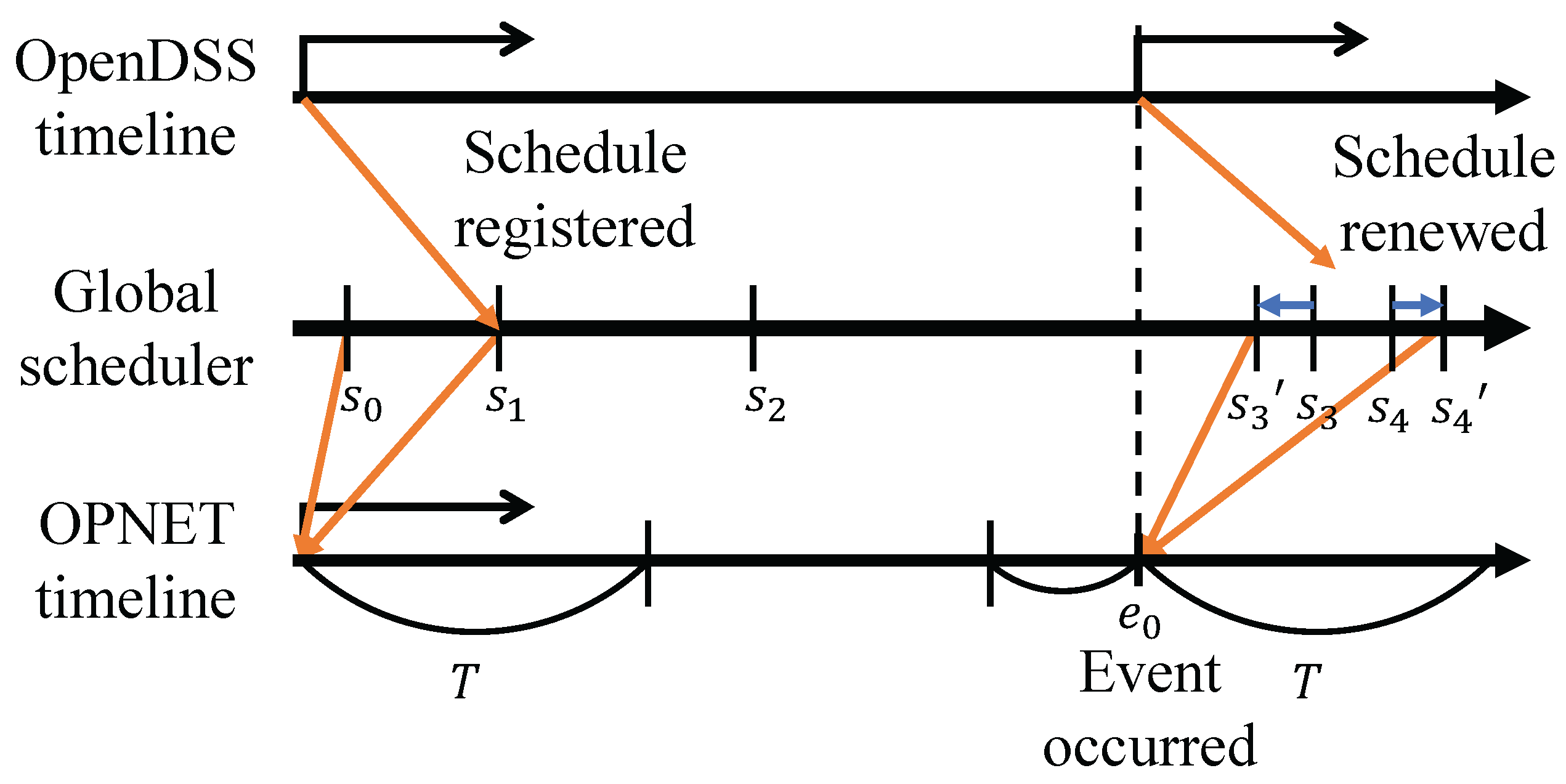
Figure 3 shows the example of the time schedule in OOCoSim. are the time of pre-defined schedules of a specific scenario, and are the time reported by OpenDSS initial simulation. The events and are transmitted to the OPNET, respectively, when the application model grants the time advance by T. OPNET simulates network event which occurs at the simulation time , and the OPNET pauses its simulation at since this event might cause the change of future plans. After re-simulating the OpenDSS from , its simulation results are reported to the application model and renews the adjusted schedules to . OPNET receives the adjusted schedules and continues simulation during T or until the other event occur.
To verify our time management scheme guarantees the time synchronism between the OPNET and the OpenDSS, it should be proved that the renewal operation of OpenDSS does not violate the time advancing status of OPNET (i.e., and ). Let be the vector of control variable at time t, then results in a set of vectors , where is an intrinsic time step parameter used in OpenDSS. In our example, results in the events at , which satisfies and . The analysis proves that the renewed schedule does not violate the time synchronism of OOCoSim timeline.
The proposed solution seems to be similar with the existing time-stepped methods because of the existence of T. However, T does not indicates the granularity of the time management, since the event handling mechanism and the adjustment of the OOCoSim schedules fully covers the time synchronism. Due to the event-driven feature of OPNET, co-simulation related events can be instantly handled independent on the variance of T.
3.3. OOCoSim Architecture and Implementation
In this subsection, we describe the architecture and implementation of OOCoSim. The most important issue of OOCoSim implementation is how to interface both simulators with user-defined application function. To implement the interfacing functionality, OOCoSim employs ESD, EI, and ESM of OPNET and also COM Interface of OpenDSS.
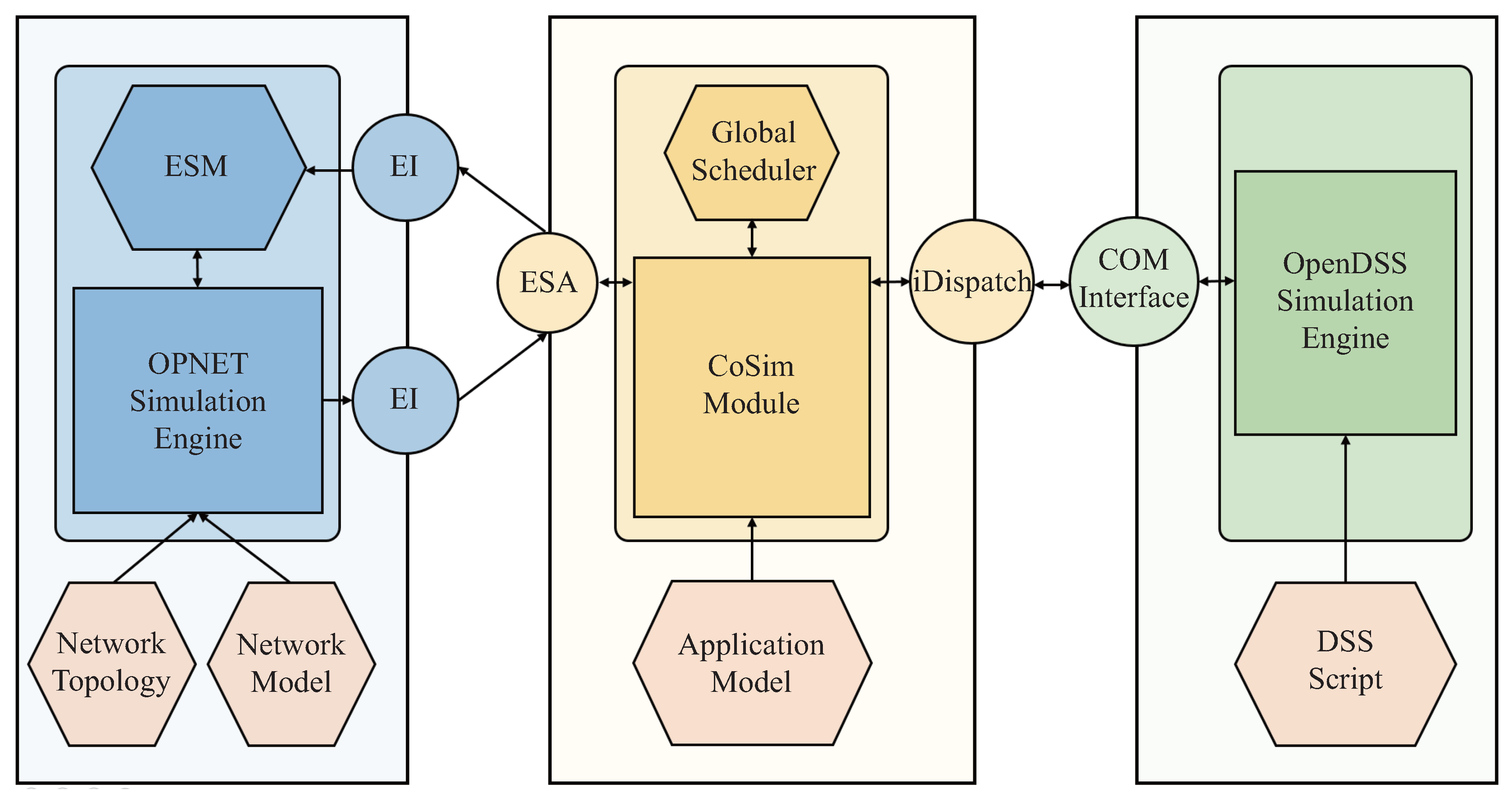
Figure 4 represents the overall architecture of OOCoSim. As we can see from the figure, the CoSim module is the most fundamental component of OOCoSim. It manages the operations of both simulators using the global scheduler and exchanges data among OPNET, OpenDSS, and the application model. The pre-defined functions of the external system access (ESA) library of OPNET are employed by the CoSim module to manage the operation of OPNET. Once OPNET simulation is activated by the CoSim module, the CoSim module and OPNET simulation communicate with each other via EIs. EIs are interfaces through which the CoSim module and OPNET simulation can access to the same information, and they are used to report network information to the CoSim module. ESM is a process model which performs protocol operations of application layer. The basic functionality of ESM is message communications. In OOCoSim, ESM is used to exchange relevant information with the CoSim module through EIs. Therefore, a supplementary state which employs EIs is added to the ESM. Specifically, OPNET collaborates with the CoSim module in the following manner.
- First, OPNET simulation is invoked by the CoSim module through the functions defined in ESA, such as Esa_Main(), Esa_Init() and Esa_Load().
- Second, message communications of the application model are defined and performed by ESM. The protocol can be implemented with a finite state machine.
- Third, the required information, such as response time and packet error, is reported to the CoSim module through the function of ESM - op_esys_interface_value_set() with the defined data type.
- Fourth, the information is retrieved by the CoSim module through the callback handler which is defined for each EI. The information is passed to the application module.
The CoSim module delivers information to OPNET and schedules an interrupt in the following manner.
- The CoSim module can execute OPNET simulation until the specific simulation time through the function Esa_Execute_Until().
- When an event occurs in OPNET simulation , the CoSim module can interrupt OPNET simulation by using the function Esa_Interrupt().
- When CoSim module receives information targeting ESM by OpenDSS or the application model, it delivers information with/without an interrupt through the functions defined in ESA such as Esa_Interface_Value_Set() and Esa_Interface_Array_Set().
OpenDSS simulation is defined by a DSS script file. The DSS script file configures a distribution system which we want to simulate and runs a simulation. Once the simulation is invoked, we can access and change the values of simulation elements through the COM interface. Therefore, we implemented CoSim module to communicate with OpenDSS simulation via the COM interface. To externally drive OpenDSS simulation: (i) we have to create DSS files to define and configure a distribution system; then (ii) we invoke the simulation with the DSS files via the COM interface; and (iii) we set/get properties of circuit elements of OpenDSS simulation. In the CoSim module, we implemented some functions that handle OpenDSS with the COM interface by C++ languages and IDispatch class of VC++, so that OOCoSim can employ OpenDSS. Specifically, OOCoSim uses IText, ICircuit, and circuit elements (e.g., ILoad and IGenerator) interfaces, all of which are subclasses of IDispatch class. The IText interface is for an execution of OpenDSS commands such as compile and clear, the ICircuit interface lets the CoSim module retrieve circuit element interfaces, and the circuit element interfaces are used to set/get the properties of the circuit element.
The OOCoSim utilizes handlers for both OPNET and OpenDSS simulation, the application model can employ user-defined interfaces of OPNET, can dispatch all the interfaces of circuit elements of OpenDSS, and can collect all the event-information of each simulator. By using the interfaces, most of operations in the smart grid application can be precisely specified in the CoSim module for the simulation study. Note that two simulators can be invoked concurrently in OOCoSim since they operate on the same platform, so that the overall simulation for those applications can be conducted in an integrated way.
4. Modeling of Smart Grid Application
In this section, we explain how the applications of the distribution and customer domains can be modeled with the demand response (DR) application. We considered a scenario in which DR application is used with a deployment of renewable energy generator.
The main problem of employing a renewable energy generator is its inherent characteristic that an environmental factor like clouds can affect its output power. This can influence on efficiency and stability of the distribution system. Therefore, in DR application, the real-time pricing is introduced to solve the problem. By providing electricity with high price when the power availability is low, the DR application tries to reduce energy consumption of each customer. To perform the DR application, we deploy the energy management system which perform rescheduling of the electricity demand of customers in the dynamics of renewable energy generation. However, in perspective of peak load distribution, an entity is required to collect all the power generation and consumption information and to determine proper electricity load of each customer since peak load distribution cannot be performed at each energy management system. Therefore, we devise the concept of gateway energy management system which can be mapped onto a service provider in the smart grid. The gateway energy management system is placed in the distribution domain and supervises the energy management of the distribution domain.
The most important point of the DR application is how to decide the electricity consumption of each customer according to the real time price. The function needs to minimize the electricity consumption cost and distributes the peak load of the distribution domain. To achieve the goal of the DR application, we simply modeled the application as follow [28]:
where and represent the real time electricity price at time t and forecasted electricity price at time , and are decision variables which represent the power demand of customer i at time t and , represents the total daily budget of each customer for electricity, T is the size of scheduling window, and N is the number of customer. The objective function indicates that the energy management system tries to minimize the electricity consumption cost by rescheduling the electricity demand of each customer. The first and second constraints represent that enough daily and instant energy consumption should be guaranteed for each customer to perform basic home tasks. The third constraint represents that the energy management system tries to find the minimum electricity consumption cost which is lower than predefined (or customer defined) budget. Totally, Equation (3) tries to minimize total energy consumption cost while consuming predefined amount of energy demand.
In our application model, when the real time and forecasted electricity prices are given, the gateway energy management system solves Equation (3) according to the given cost. Then, the optimal value of electricity load is distributed to each energy management system to control their electricity. In the next section, we will present how this DR application model can be modeled into OOCoSim and can be simulated through OOCoSim. Moreover, we will precisely investigate whether OOCoSim can produce the proper simulation results.
5. Simulation Study
In this section, we establish a simulation scenario for OOCoSim based on the model described in Section 4. Then, the simulation results are provided with detailed explanations.
5.1. Simulation Model
Power System: The distribution system can be defined in OpenDSS through the DSS script. To perform simulation study of the DR application with OOCoSim, we configured IEEE 13 Node and 34 Node test feeder system as a target distribution system through the DSS scripts. On each distribution system, we placed the wind generator to simulate the impact of the dynamics of the Distributed Energy Resource (DER). However, determining the location and the output power of DER is an important issue because it highly impacts the technical benefits of distributed power system such as the power loss. There has been a lot of research to solve this problem [29,30]. Especially, A. Anwar and H.R. Pota [29] proposed an algorithm to identify the appropriate location and size (output power) of a distributed generator. At first, the algorithm calculates the sensitivity factor of each bus, where . The sensitivity factor represents the change in power loss () of specific bus () when the size of distributed generation is varied from to . After listing the most sensitive buses, the algorithm calculates the power loss for large variation of DER size in each bus. The power loss curves are almost a quadratic function [31], and the algorithm picks the bus and the size which give the minimum power loss. According to the analyses in [29], we installed the wind generator at bus 675 in 13 Node and at bus 844 in 34 Node system whose output power are 1.29 MW and 1.15 MW, respectively. Figure 5 is a graphical representation of the configured distribution system.
Moreover, to consider the output diversity of the power generator, we made a probable profile for the generator in the period of 5 min according to the wind power data at Seoul, Korea, from 9 September, 09:56 to 10:00 [32] in which {4,1,0,8,2,0,4,5} m/s of wind speed are reported at each time point of {09:56,09:59,09:58,09:59,10:00}. We simply assumed that the output power of the wind generation is proportional to the wind power as , where represents actual output power of the wind generator and is the reference output power (1.29 MW for the 13 node system and 1.15 MW for the 34 node system). Figure 6 depicts the assumed output profile of the wind generator.
We modified the 34 Node system by reducing each line length down to 10% since the original 34 Node system is too large to be used together with the traditional WLAN coverage.
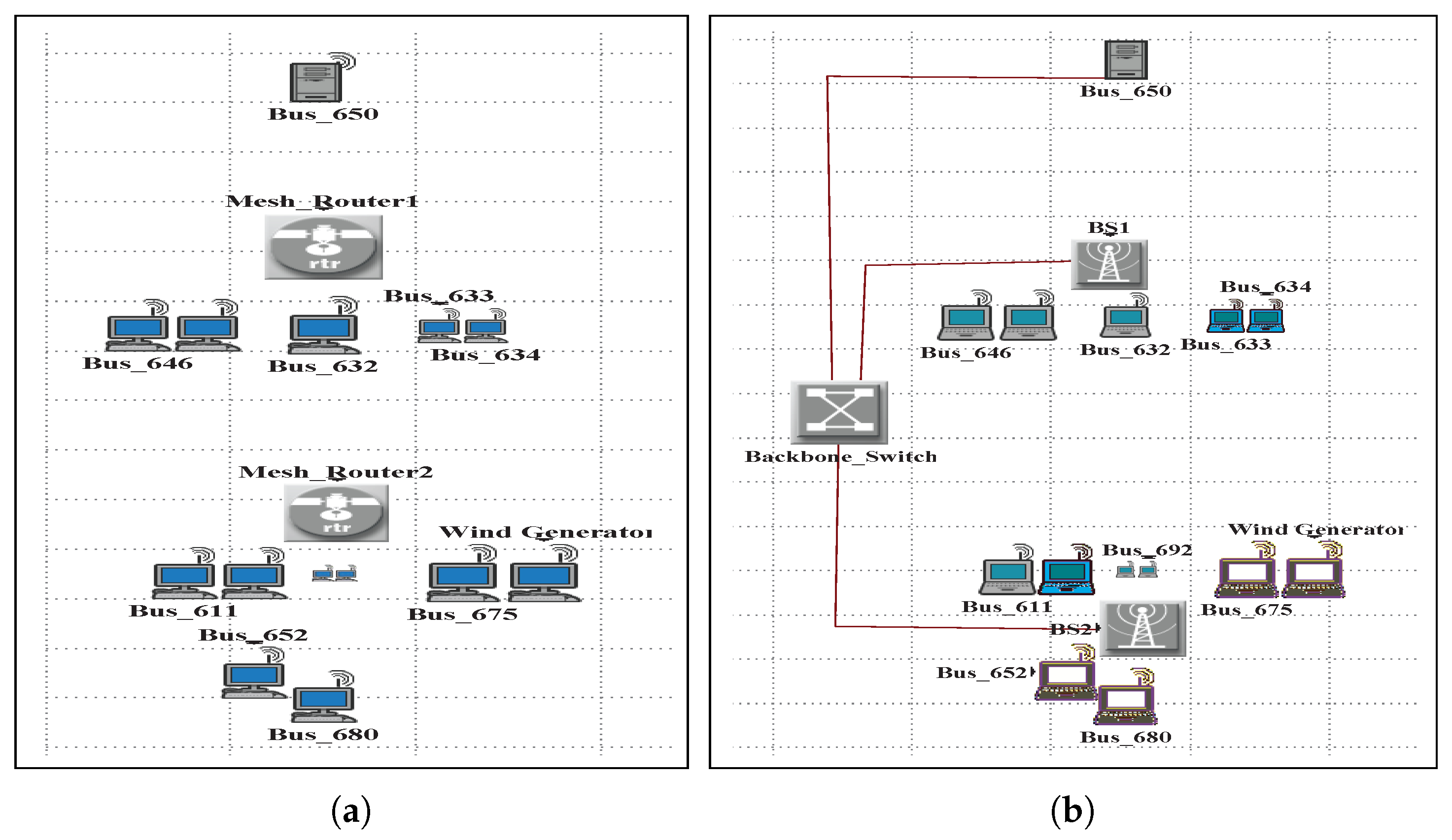
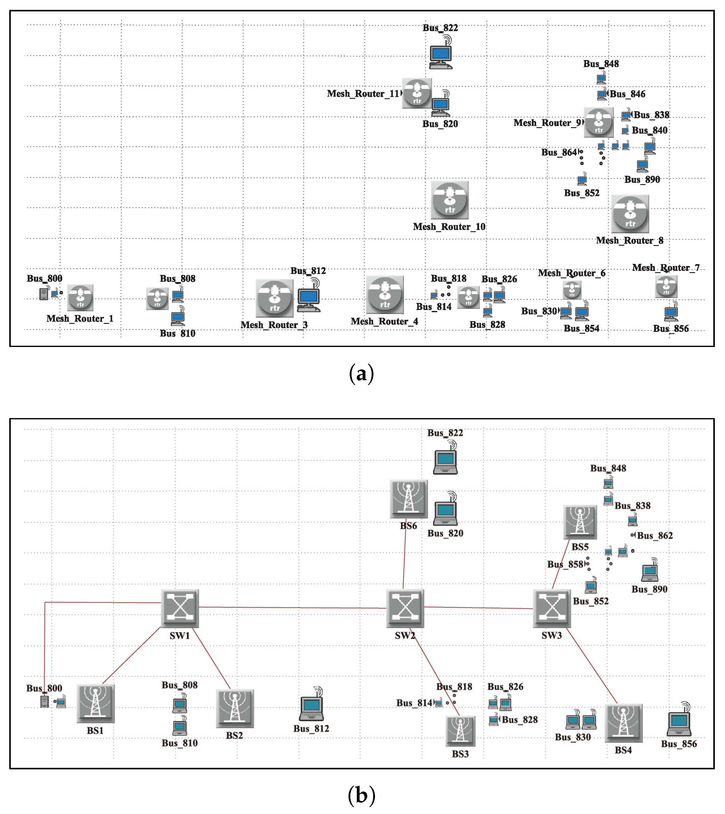
Network System: The next step to simulate the smart grid application is to model the network infrastructure. We assumed that there exists an energy management system at each bus. We mapped the topology of the target distribution system into OPNET network topology. Figure 7 and Figure 8 present the network system of 13 Node and 34 Node in OPNET.
To verify the impact of the networking system, we employed two network systems for the distribution system: the one with a WLAN Mesh topology (Figure 7a and Figure 8a), and the other with a combined topology of WiMAX and Ethernet backbone (Figure 7b and Figure 8b). The network topology of each system was designed considering the practical feature of communication devices. For example, the distance between the bus 650 and the bus 632 is about 610 m, while the distance between the bus 632 and the bus 645 or the bus 633 is about 152 m, according to [33]. Since increasing the communication range for only one node could lead to the inefficient design of the wireless network, we connected the energy management system of bus 650 to the backbone network (WiMAX) or the mesh router (WLAN Mesh). Then, the APs (WLAN Mesh) or the BSs (WiMAX) are deployed to connect the wireless devices running the enenrgy management system for each bus.
We modeled the network system with server/client model. The gateway energy management system acts as a server and the other energy management systems perform the role of a client. The specific configuration for each node is as follows:
- The gateway energy management system is a wlan_server or ethernet_server node model in OPNET.
- The energy management system model is a node model which includes the ESM process, and each ESM process reports the response time of application traffic to the CoSim module;
- The communications between the gateway system and each energy management system are configured with a server/client model.
As the operational scenario, each energy management system sends a request message whose size is 1 KB every second, and the gateway sends a response message whose size is 5 KB to the energy management system. When the energy management system receives the response message, it calculates the response time and inform the result to the CoSim module.
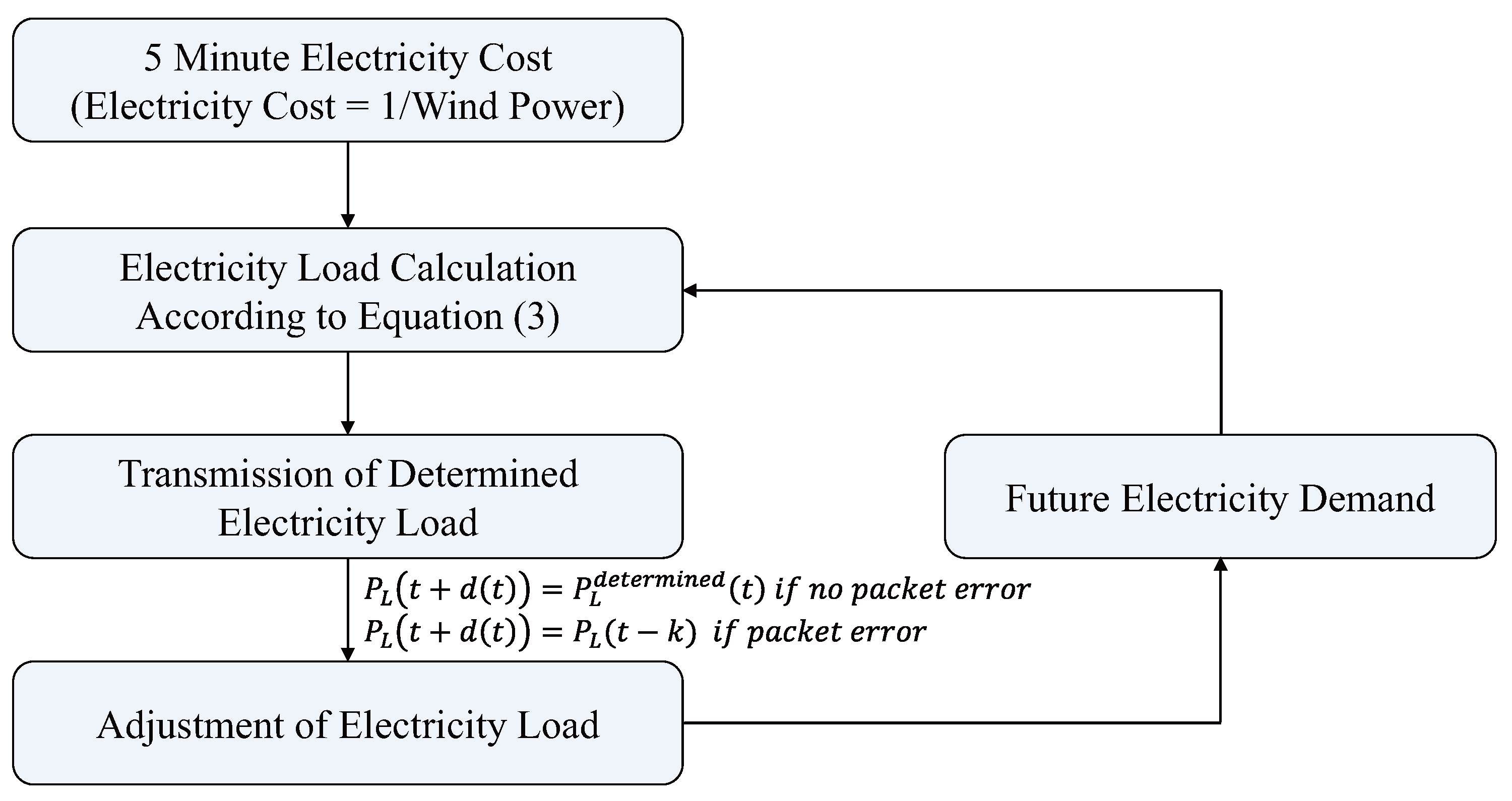
Smart Grid Application: We also implemented the application model in the CoSim module. In Section 4, we formulated the energy management system operation. We simply assumed that electricity forecasting is performed at each five minute, and the price of electricity is inversely proportional to the output power of the wind generator. Therefore, T in Equation (3) is set to 300 s, the k is set to 1 s, and .
The forecasted electricity price is delivered to the gateway energy management system, and it decides the second-level electricity load of each energy management system by solving Equation (3). Every second, each energy management system requests its actual load to the gateway energy management system and it adjusts their load. Since the gateway energy management system calculates the load of each customer according to the forecasted output power of the wind generator, it might recalculate the load value if the actual output power is changed. However, we simply assume that the forecasted wind power is correct and the load calculation is performed only once every five min.
The retrieval of the actual load of each customer is performed through the network infrastructure, there might exist the network delay and packet error. Therefore, the CoSim module should schedule the load adjustment event according to the following equation,
where is a determined load of customer i for t second, and is a communication delay of the load decision message for customer i at time t.
Figure 9 summarizes the operation flow of the DR application. Note that traditionally, DR is performed for a long period of time and as a prearranged plan, for instance, 1-day early or 1-hour early. However, as the advanced computing and networking technologies are applied to the power system, the scale of the DR is being shortened. Recently, many studies have proposed and verified the impact of load scheduling at minute-level or second-level [34,35]. Therefore, we do not regard the defined application model as an unrealistic model but as a future application model in the smart grid.
5.2. Simulation Results
We conducted the simulation as follows:
- OOCoSim creates events for the wind generator according to the pre-defined wind generator profile.
- The CoSim module calculates the load based on the forecasted 5 min electricity cost information.
- Every second, OOCoSim makes message communications through OPNET simulation and receives the response time information of each bus.
- Based on the calculated load and the response time information, CoSim module creates new events for OpenDSS simulation and assigns them to the global scheduler.
- When the scheduler encounters OpenDSS event, it applies the event to OpenDSS.
- After each event is applied to OpenDSS, OOCoSim dispatches the distribution system information—the total power loss and voltage.
In our simulation study, we used energy consumption data of Almanac of Minutely Power Dataset-AMPds [36], which provides minute-level observed electricity metering data. We compared the impact of the DR application with the data. The tagging “w/o DR” in the following figures and tables represents the results of the profile which follows AMPds data.
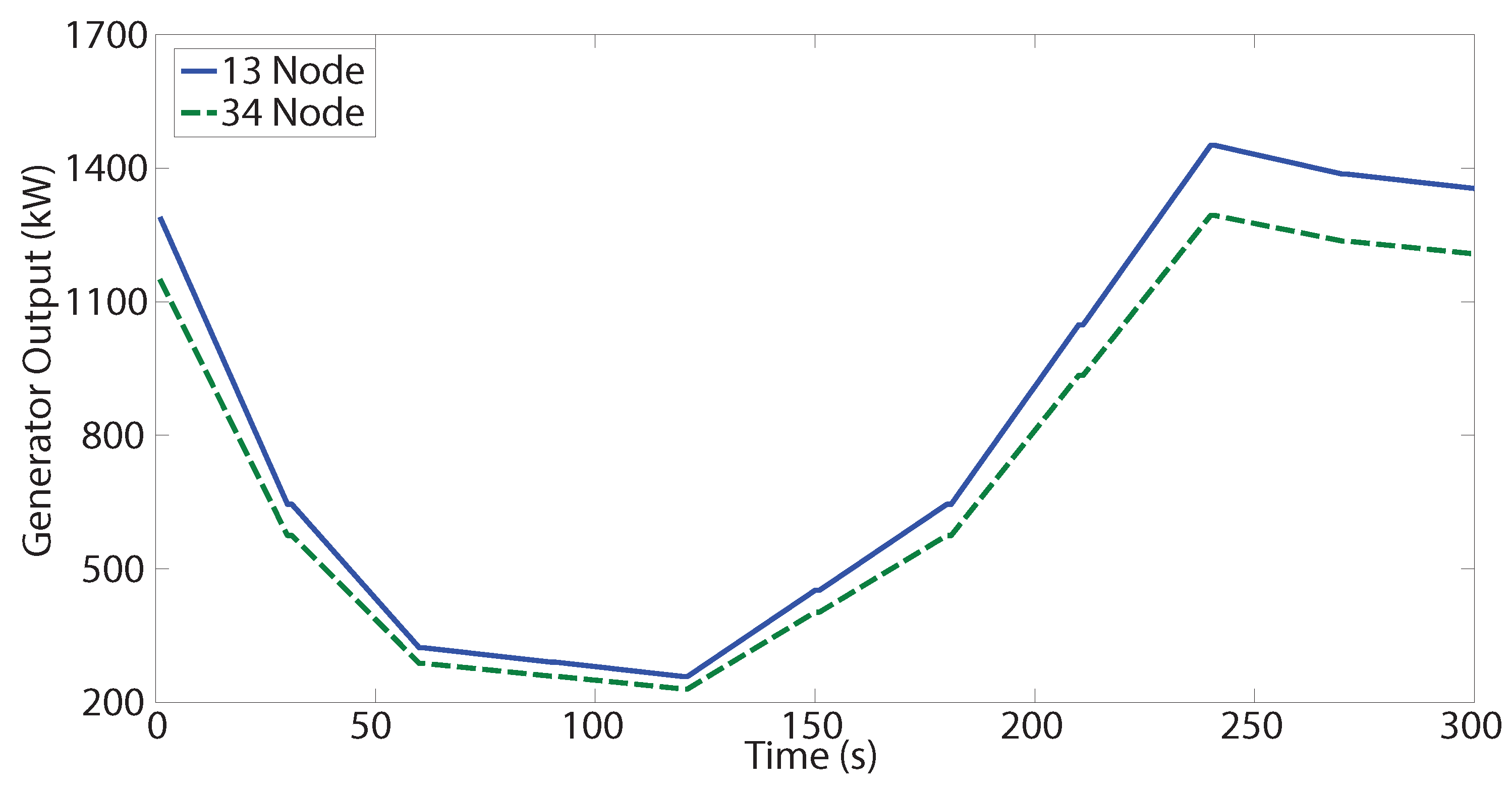
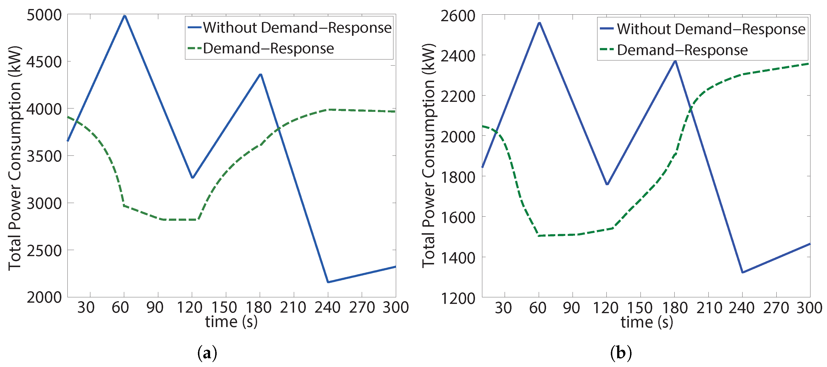
Table 1 denotes total energy consumption cost during 5 min, and Figure 10 describes the power consumption of the 13 and 34 node system. We can easily note from the table that the DR model achieved its goal—minimizing the electricity usage cost. In both systems, we could save approximately 15% of electricity usage cost while consuming the same amount of electricity energy. Moreover, through Figure 10, we can also note that the application also achieved its another goal—distributing the peak load. Based on the results, we can conclude that the application tried to use large amount of the electricity when the electricity price is cheap and it also uses small amount of the electricity when the electricity price is expensive while successfully minimizing the total budget of electricity consumption and distributing the peak load.
The next step is to consider the following questions “How the DR application affects the distribution system?” and “How the underlying network system affects the performance of the DR application?” These are more important questions to analyze in the smart grid where the power system and IT infrastructure are tightly coupled. To answer these questions, we analyzed the impact of the DR application in perspective of the power loss and voltage of the distribution system. To represent the impact of the networking system, we devised an ideal network scenario where the network delay and the packet error rate are 0.
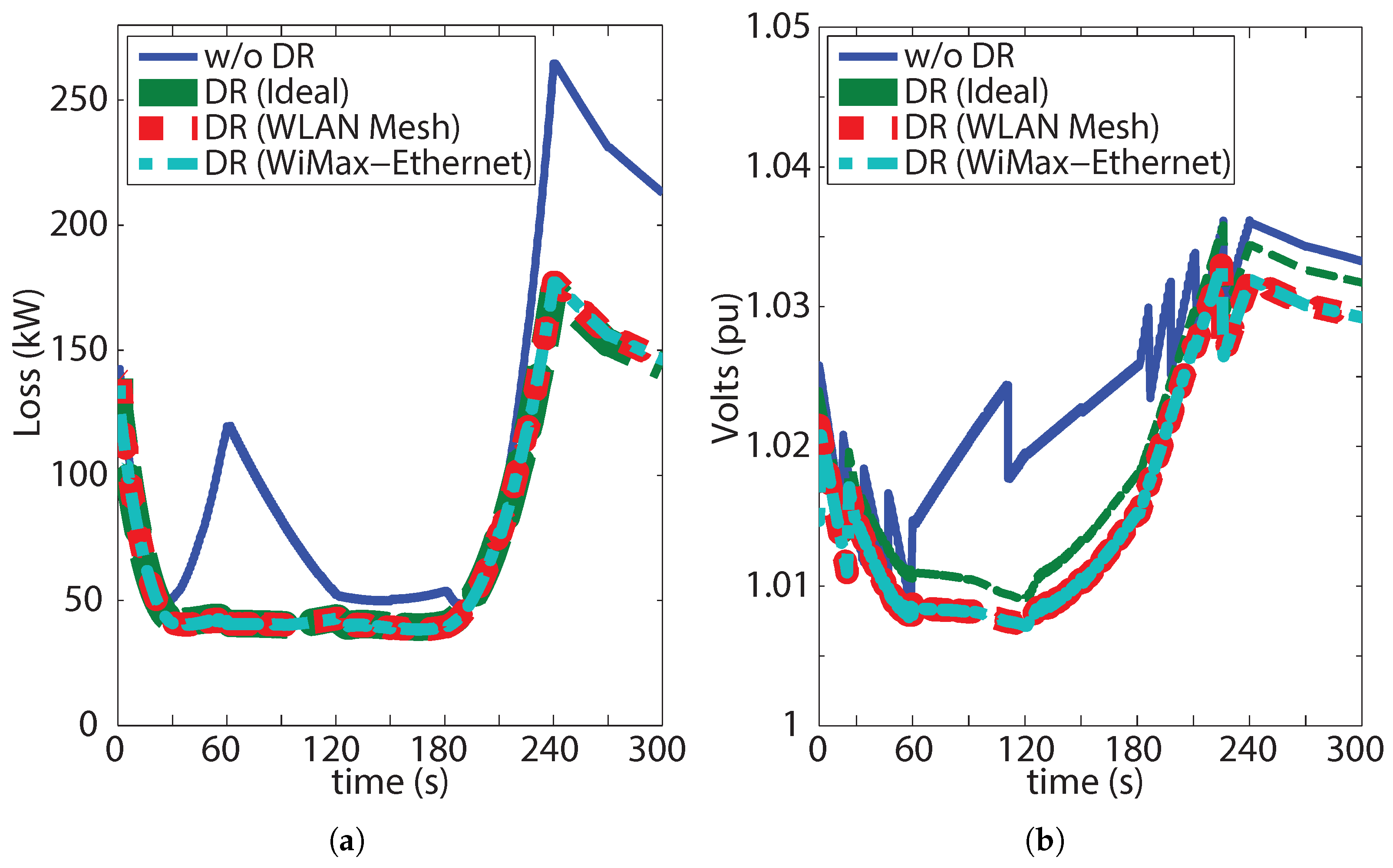
Figure 11a shows the power loss of the 13 Node system. We can observe that if we enable energy management function, we can obtain much benefit in perspective of the power loss since the lines tagged with “DR” shows much lower power loss than that of “w/o DR”. A notable point is that through the DR application, small power loss can be achieved when the output power of the renewable energy generation is very low (from 60 s to 180 s). Since deficient energy provision can lead serious results such as “blackout”, it is much more important to reduce power loss when power availability is very low. Therefore, we can conclude that the real time price based DR application contributed greatly to stability and efficiency of the distribution system in our simulation study. On the other hand, Figure 11b shows the voltage profile of the bus 652 at which the voltage is increased mostly when we do not use energy management functions. We can identify from the results that the energy management function can also contribute to the stability of the distribution grid since the lines tagged with “DR” have values closer to the voltage of 1 pu. Note that the “pu” means the fraction of actual voltage to defined base voltage. As the actual voltage gets closer to the base voltage (i.e., 1 pu), the system can be regarded as a more stable system. Table 2 describes the total power loss and the voltage index of the 13 Node system for 5 min. From the results we can note that through the DR application, the power loss can be reduced and the voltage stability of the distribution system can be maintained.
By observing the results, we can conclude that the designed DR application can successfully contribute to stable and efficient distribution system. A notable point of the simulation results of Figure 11a,b and Table 2 is that the impact of the underlying network infrastructure is relatively small. Since the 13 node system is very a small system, the performance gap between the two network systems is very small, and it causes little differences of the simulation results. We can note that both WLAN network and WiMAX network scenarios tend to converge to the ideal network scenario.
However, when we conducted a simulation with 34 Node system, we can precisely see to what extent the network performance affects the distribution system. Because the 34 Node system is a much more large system than the 13 Node system, there exists much greater differences between the application performance of WLAN Mesh and WiMax-Ethernet backbone network. Figure 12a shows the total power loss that we simulated from the 34 Node system. Basically, the DR application also could achieve its goal in 34 Node system. However, there exists large difference between the WiMax-Ethernet backbone and WLAN Mesh network. Since the 34 node system consists of many energy management systems, the probability of packet collision was seriously increased. It led the performance degradation of the DR application. Moreover, a number of packets were dropped due to the multi-hop transmissions, which led the unexpected result. However, the WiMax-Ethernet backbone network shows almost similar performance to the ideal scenario. Figure 12b shows the voltage of the 852 bus in the 34 Node system. We can see that the energy management function can successfully maintain the distribution system stable. However, when we employed WLAN Mesh network, we cannot achieve grid stability since the network has poor connectivity and few energy management systems receive the control information in desirable time.
Table 3 shows the total power loss and voltage index of the 34 node system. The application which employs WLAN Mesh network system shows larger power loss and higher voltage index value. Therefore, we can conclude that to employ WLAN based backbone for DR application in the 34 node system, a new protocol which can resolve the low connectivity issue should be designed. For example, modified MAC protocols or routing schemes, which can guarantee high delivery ratio in multi-hop wireless network, should be introduced to construct WLAN based backbone network.
In addition, we analyzed the transmission delay of network packet in each scenario. The transmission delay of the smart grid network is one of the critical issue since an excessive delay of the power state report could lead to the delayed control of the power distribution, which results in the unexpected power loss. We ran the OOCoSim simulation for each scenario (13 and 34 node system and WLAN Mesh and WiMAX network system) for 600 s and collected packet response provided from the OPNET in each simulation. Figure 13 shows the CDF of the transmission delay of the simulations. As shown in Figure 13, WiMAX-Ethernet shows almost similar distribution of transmission delay which has about 0.1 s at 99% probability in the 13 node and the 34 node cases, while WLAN Mesh shows over 1 s at 70% probability in the 34 node system. However, 13 node WLAN Mesh system shows lower delay in the 13 node case. The evaluation shows that WLAN Mesh network system performs lower delay communication than WiMAX-ethernet network system in smaller network, and WiMAX-ethernet network system could be suitable choice for large-scale and delay-constrained smart grid application.
Based on all the simulation results, we can confirm that the proposed OOCoSim can successfully conduct the simulation for the smart grid where the power grid and the communication infrastructure are tightly coupled with each other. Additionally, we can also realize that we can use OOCoSim to see how the underlying network affects the power grid.
5.3. Discussions on Simulation Scalability and Stability
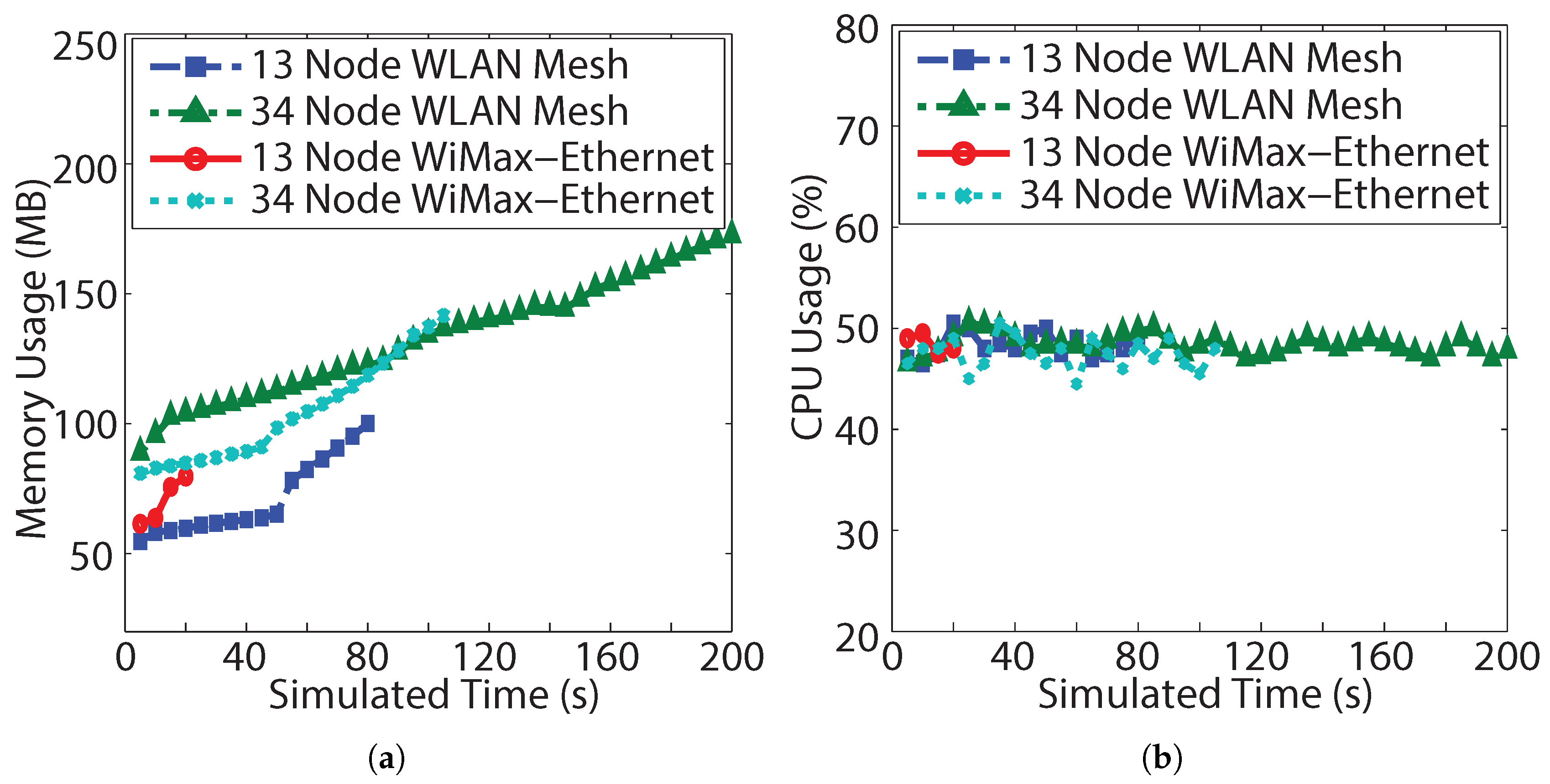
Table 4 summarizes execution time of simulation study using a computing system which has core2 duo 2.4 GHz CPU and 8 GB physical memory. The simulation time was 600 s for each scenario and network topology. Basically, in WLAN Mesh network scenarios, many more events were generated and processed in OPNET due to the CSMA/CA based channel access and multi-hop transmission, and therefore, longer execution time was reported. In addition, the number of events of OpenDSS is smaller in WLAN Mesh network because its poor network performance created fewer number of application events. We can observe that the execution time of both simulation tool is well proportional to the number of events. Although the number of events can differ according to the simulation configuration, the linearity can guarantee the scalability of the simulation [26]. Therefore, we can conclude that the both simulation tools have enough scalability to perform simulation on the smart grid application. Figure 14a represents the usage of memory resource for the scenarios described in previous subsection. We can observe that OOCoSim has a linearly increasing pattern of the memory usage for all scenarios. The linearity can guarantee that simulations of the smart grid application can be performed within expected size of memory resource [37]. Therefore, we can conclude that OOCoSim is scalable and stable in the perspective of memory usage. The cpu usage of OOCoSim is represented in Figure 14b. For four scenarios, stable cpu usage pattern in which most of values are positioned between 44% and 52% was reported. The results indicate that regardless of the configuration of simulations, OOCoSim requires similar amount of CPU usage, therefore, OOCoSim can perform stable and sustainable simulations for applications in distribution and customer domain.
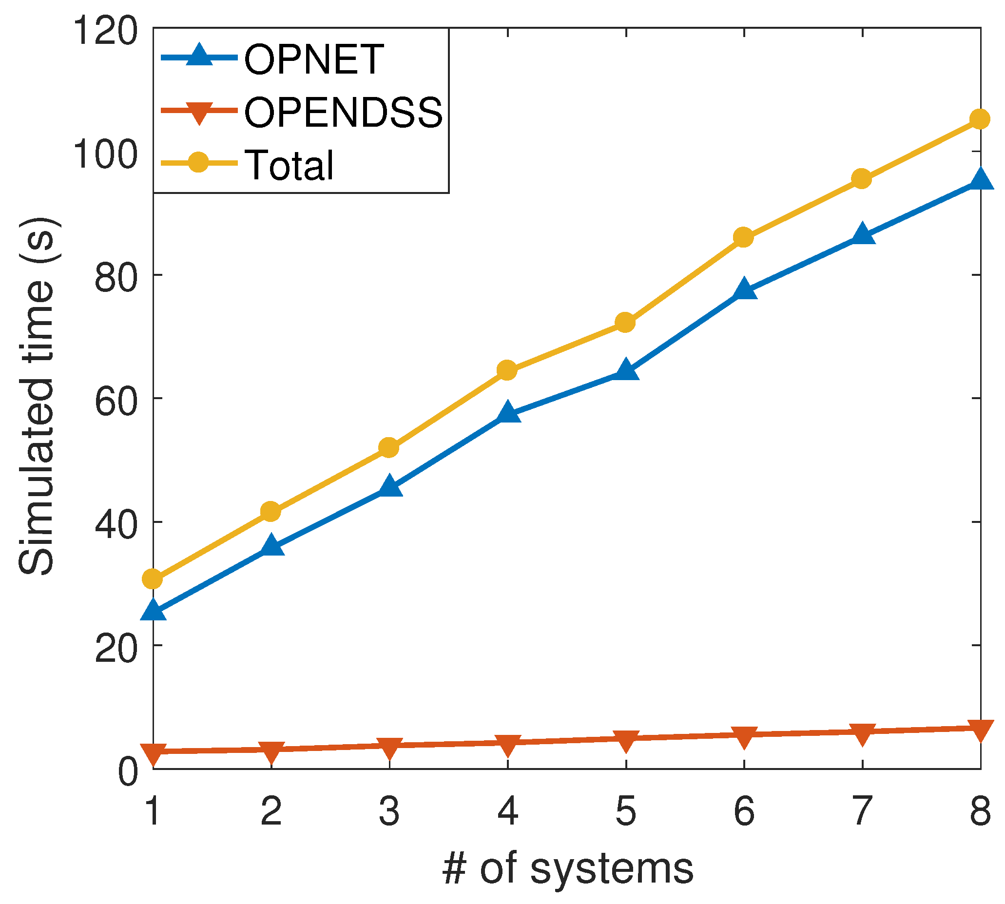
To verify the scalability of the simulation system further, we duplicated 13 node WiFi Mesh system for two to eight times and ran each case. Since OpenDSS only can run a single circuit, we utilized Direct connection Shared Library for OpenDSS. With this engine, multiple OpenDSS simulations can be executed in parallel. Figure 15 shows the simulation time of OPNET, OpenDSS, and the total simulation time including OOCoSim operations with respect to the number of 13 node WiFi Mesh systems. As shown in Figure 15, OPNET simulation highly accounts for a high proportion of the total simulation time. In addition, since OpenDSS can simulate multiple circuits concurrently, the simulated time of OpenDSS grows much slower than OPNET. Regardless of the proportion of the simulation time, Figure 15 shows that the total simulation time of OOCoSim linearly increases as the number of system increases. The observation shows that OOCoSim has enough scalability to perform the simulation on the smart grid system and its application.
6. Conclusions and Future Work
In this paper, we proposed a cosimulation system, OOCoSim, for smart grid applications in the distribution and customer domain. We described the basic concept, design, and implementation of OOCoSim. Moreover, we conducted a simulation study for the demand response application which is a representative application of distribution and customer domain in smart grid. With the proposed OOCoSim, we can carry out an extensive simulation study for the smart grid, and we can have the right direction of building a smart grid.
Acknowledgments
This research was supported in part by Basic Science Research Program through the National Research Foundation of Korea (NRF) funded by the Ministry of Education (NRF-2015R1D1A1A01059151), and in part by “Human Resources program in Energy Technology” of the Korea Institute of Energy Technology Evaluation and Planning (KETEP) granted financial resource from the Ministry of Trade, Industry & Energy, Republic of Korea (No. 20154030200610).
Author Contributions
Hwantae Kim designed the overall architecture of OOCoSim and the simulation models. Kangho Kim implemented the system of OOCoSim and analyzed the result of the simulation studies. Seongjoon Park designed the global time management module of OOCoSim and analyzed the synchronism of the system. Hwantae Kim, Kangho Kim and Seongjoon Park contributed equally to this work. Hyunsoon Kim surveyed the related works of OOCoSim and examined the contents of the paper. Hwangnam Kim governed the overall procedure of this research.
Conflicts of Interest
The authors declare no conflict of interest. The founding sponsors had no role in the design of the study; in the collection, analyses, or interpretation of data; in the writing of the manuscript, and in the decision to publish the results.
References
- Albano, M.; Ferreira, L.L.; Pinho, L.M. Convergence of smart grid ict architectures for the last mile. IEEE Trans. Ind. Inf. 2015, 11, 187–197. [Google Scholar] [CrossRef]
- Bae, M.; Kim, K.; Kim, H. Preserving privacy and efficiency in data communication and aggregation for ami network. J. Netw. Comput. Appl. 2016, 59, 333–344. [Google Scholar] [CrossRef]
- Son, H.; Kang, T.Y.; Kim, H.; Roh, J.H. A secure framework for protecting customer collaboration in intelligent power grids. IEEE Trans. Smart Grid. 2011, 2, 759–769. [Google Scholar] [CrossRef]
- Kim, K.; Kim, H.; Jung, J.; Kim, H. Afar: A robust and delay-constrained communication framework for smart grid applications. Comput. Netw. 2015, 91, 1–25. [Google Scholar] [CrossRef]
- Anderson, K.; Du, J.; Narayan, A.; El Gamal, A. Gridspice: A distributed simulation platform for the smart grid. IEEE Trans. Ind. Inf. 2014, 10, 2354–2363. [Google Scholar] [CrossRef]
- Locke, G.; Gallagher, P.D. Nist Framework and Roadmap for Smart Grid Interoperability Standards, Release 3.0; National Institute of Standards and Technology: Gaithersburg, MD, USA, 2014. [Google Scholar]
- Parikh, P.P.; Kanabar, M.G.; Sidhu, T.S. Opportunities and challenges of wireless communication technologies for smart grid applications. In Proceedings of the 2010 IEEE Power and Energy Society General Meeting, Providence, RI, USA, 25–29 July 2010. [Google Scholar]
- Sadi, M.A.H.; Ali, M.H.; Dasgupta, D.; Abercrombie, R.K. Opnet/simulink based testbed for disturbance detection in the smart grid. In Proceedings of the 10th Annual Cyber and Information Security Research Conference, Oak Ridge, TN, USA, 7–9 April 2015. [Google Scholar]
- Sarena, S.T. A Framework for Microgrid Analysis Using OpenDSS; LAP LAMBERT Academic Publishing: Saarbrücken, Germany, 2014. [Google Scholar]
- Hopkinson, K.; Wang, X.; Giovanini, R.; Thorp, J.; Birman, K.; Coury, D. Epochs: A platform for agent-based electric power and communication simulation built from commercial off-the-shelf components. IEEE Trans. Power Syst. 2006, 21, 548–558. [Google Scholar] [CrossRef]
- Lin, H.; Veda, S.S.; Shukla, S.S.; Mili, L.; Thorp, J. Geco: Global event-driven co-simulation framework for interconnected power system and communication network. IEEE Trans. Smart Grid 2012, 3, 1444–1456. [Google Scholar] [CrossRef]
- Kilic, N.; Gungor, V.C. Analysis of low power wireless links in smart grid environments. Comput. Netw. 2013, 57, 1192–1203. [Google Scholar] [CrossRef]
- Karimi, B.; Namboodiri, V.; Aravinthan, V.; Jewell, W. Feasibility, challenges, and performance of wireless multi-hop routing for feeder level communication in a smart grid. In Proceedings of the 2nd International Conference on Energy-Efficient Computing and Networking, New York, NY, USA, 31 May–1 June 2011; pp. 31–40. [Google Scholar]
- Karnouskos, S.; De Holanda, T.N. Simulation of a smart grid city with software agents. In Proceedings of the Third UKSim European Symposium on Computer Modeling and Simulation, Athens, Greece, 25–27 November 2009; pp. 424–429. [Google Scholar]
- Godfrey, T.; Mullen, S.; Dugan, R.; Rodine, C.; Griffith, D.; Golmie, N. Modeling smart grid applications with co-simulation. In Proceedings of the 2010 First IEEE International Conference on Smart Grid Communications, Gaithersburg, MD, USA, 4–6 October 2010; pp. 291–296. [Google Scholar]
- Lin, H.; Sambamoorthy, S.; Shukla, S.; Thorp, J.; Mili, L. Power system and communication network co-simulation for smart grid applications. In Proceedings of the 2011 IEEE PES Innovative Smart Grid Technologies (ISGT), Anaheim, CA, USA, 17–19 January 2011; pp. 1–6. [Google Scholar]
- Bhor, D.; Angappan, K.; Sivalingam, K.M. Network and power-grid co-simulation framework for smart grid wide-area monitoring networks. J. Netw. Comput. Appl. 2016, 59, 274–284. [Google Scholar] [CrossRef]
- Mets, K.; Verschueren, T.; Develder, C.; Vandoorn, T.L.; Vandevelde, L. Integrated simulation of power and communication networks for smart grid applications. In Proceedings of the 2011 IEEE 16th International Workshop on Computer Aided Modeling and Design of Communication Links and Networks (CAMAD), Kyoto, Japan, 10–11 June 2011; pp. 61–65. [Google Scholar]
- Tong, X. The co-simulation extending for wide-area communication networks in power system. In Proceedings of the 2010 Asia-Pacific Power and Energy Engineering Conference (APPEEC), Chengdu, China, 28–31 March 2010. [Google Scholar]
- Mallouhi, M.; Al-Nashif, Y.; Cox, D.; Chadaga, T.; Hariri, S. A testbed for analyzing security of scada control systems (tasscs). In Proceedings of the 2011 IEEE PES Innovative Smart Grid Technologies (ISGT), Anaheim, CA, USA, 17–19 January 2011. [Google Scholar]
- Sun, X.; Chen, Y.; Liu, J.; Huang, S. A co-simulation platform for smart grid considering interaction between information and power systems. In Proceedings of the 2014 IEEE PES Innovative Smart Grid Technologies Conference (ISGT), Washington, DC, USA, 19–22 February 2014. [Google Scholar]
- Dugan, R.C. OpenDSS Reference Guide; Electric Power Research Institute, Inc.: Palo Alto, CA, USA, 2012. [Google Scholar]
- Microsoft MSDN. Available online: http://msdn.microsoft.com/en-us/library/ms680573 (accessed on 8 January 2018).
- Hamida, E.B.; Chelius, G.; Gorce, J.-M. Impact of the physical layer modeling on the accuracy and scalability of wireless network simulation. Simulation 2009, 85, 574–588. [Google Scholar] [CrossRef] [Green Version]
- Dricot, J.-M.; Doncker, P.D. High-accuracy physical layer model for wireless network simulations in ns-2. In Proceedings of the IWAN’04–International Workshop on Wireless Ad-hoc Networks, Oulu, Finland, 31 May–3 June 2004. [Google Scholar]
- Montenegro, D.; Hernandez, M.; Ramos, G. Real time opendss framework for distribution systems simulation and analysis. In Proceedings of the 2012 Sixth IEEE/PES on Transmission and Distribution: Latin America Conference and Exposition (T&D-LA), Montevideo, Uruguay, 3–5 September 2012. [Google Scholar]
- Li, W.; Ferdowsi, M.; Stevic, M.; Monti, A.; Ponci, F. Cosimulation for smart grid communications. IEEE Trans. Ind. Inf. 2014, 10, 2374–2384. [Google Scholar] [CrossRef]
- Chen, L.; Wu, Z.; Fu, Y. Real-time price-based demand response management for residential appliances via stochastic optimization and robust optimization. IEEE Trans. Smart Grid 2012, 3, 1822–1831. [Google Scholar] [CrossRef]
- Anwar, A.; Pota, H. Loss reduction of power distribution network using optimum size and location of distributed generation. In Proceedings of the 2011 21st Australasian Universities Power Engineering Conference (AUPEC), Brisbane, Australia, 25–28 September 2011. [Google Scholar]
- Lamaina, P.; Sarno, D.; Siano, P.; Zakariazadeh, A.; Romano, R. A model for wind turbines placement within a distribution network acquisition market. IEEE Trans. Ind. Inf. 2015, 11, 210–219. [Google Scholar] [CrossRef]
- O’Donnell, J. Voltage Management of Networks With Distributed Generation. Ph.D. Thesis, The University of Edinburgh, 2008. Available online: http://hdl.handle.net/1842/2577 (accessed on 8 January 2018).
- Korea Meteorological Administration. Automatic Weather Station. 2013. Available online: http://www.kma.go.kr/weather/observation/currentweather.jsp (accessed on 8 January 2018).
- Kersting, W.H. Radial distribution test feeders. In Proceedings of the 2001 IEEE Power Engineering Society Winter Meeting, Columbus, OH, USA, 28 January–1 February 2001; Volume 2, pp. 908–912. [Google Scholar]
- SIMENS. Automated Demand Response Using OpenADR Application Guide, 3rd ed.; SIMENS: Berlin/Munich, Germany, 2011. [Google Scholar]
- Taylor, J.W. An evaluation of methods for very short-term load forecasting using minute-by-minute british data. Int. J. Forecast. 2008, 24, 645–658. [Google Scholar] [CrossRef]
- Makonin, S. The Almanac of Minutely Power Dataset. 2013. Available online: http://ampds.org/ (accessed on 8 January 2018).
- Fujimoto, R.M.; Perumalla, K.; Park, A.; Wu, H.; Ammar, M.H.; Riley, G.F. Large-scale network simulation: How big? how fast? In Proceedings of the 11th IEEE/ACM International Symposium on Modeling, Analysis and Simulation of Computer Telecommunications Systems (MASCOTS), Orlando, FL, USA, 12–15 October 2003; pp. 116–123. [Google Scholar]
Figure 1.
The conceptual representation of the proposed cosimulation.

Figure 2.
The finite state machine of the cosimulation.
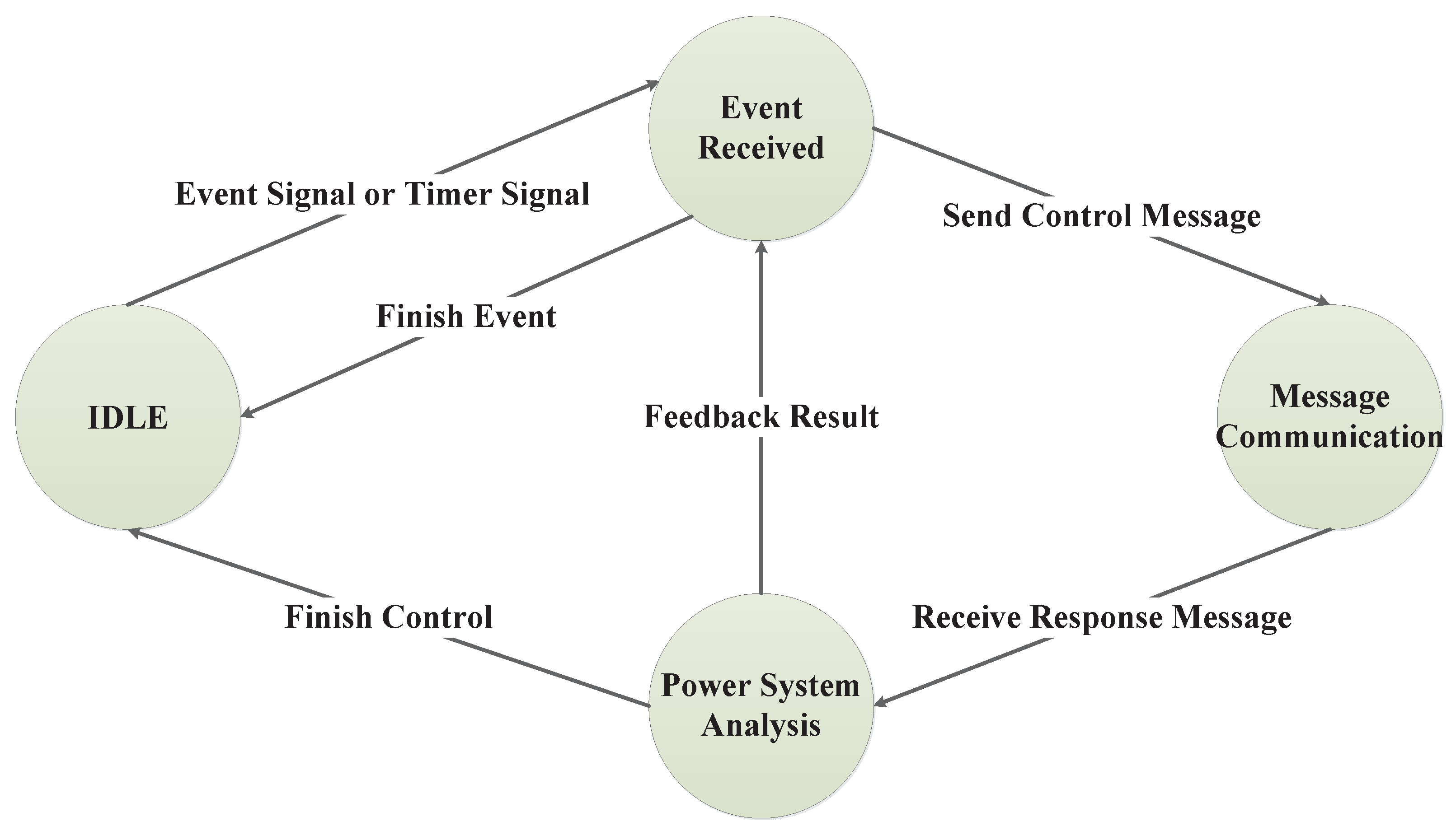
Figure 3.
The example case of the scheduling mechanism.

Figure 4.
The OOCoSim architecture.

Figure 5.
IEEE Node Test Feeder with local wind generator. (a) IEEE 13 Node Test Feeder; (b) IEEE 34 Node Test Feeder.
Figure 5.
IEEE Node Test Feeder with local wind generator. (a) IEEE 13 Node Test Feeder; (b) IEEE 34 Node Test Feeder.
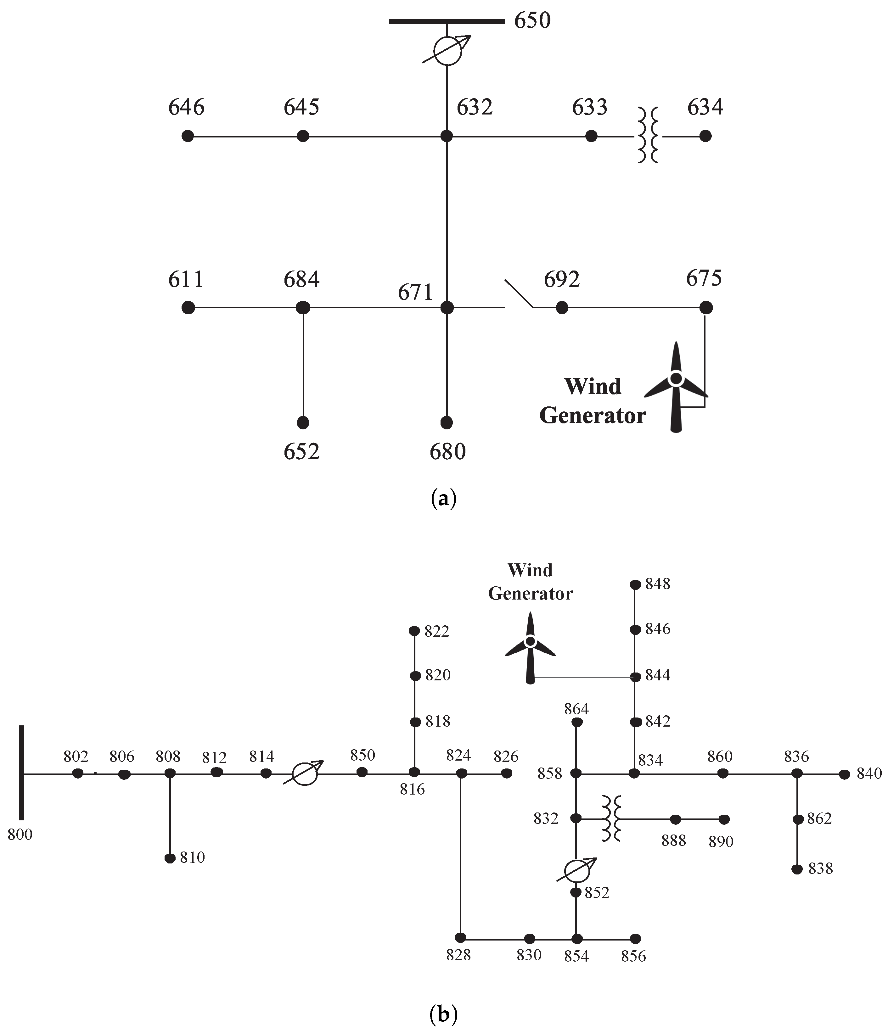
Figure 6.
The assumed output power of the wind generator.

Figure 7.
The modeled network topologies of 13 Node. (a) 13 Node WLAN Mesh; (b) 13 Node WLAN WiMax.

Figure 8.
The modeled network topologies of 34 Node. (a) 34 Node WLAN Mesh; (b) 34 Node WLAN WiMax.

Figure 9.
The operational flow of the application model.

Figure 10.
The power consumption in 13 and 34 node systems. (a) 13 Node system; (b) 34 Node system.

Figure 11.
The power loss and the voltage of 13 Node system. (a) Total power loss; (b) Voltage of 652 bus.
Figure 11.
The power loss and the voltage of 13 Node system. (a) Total power loss; (b) Voltage of 652 bus.

Figure 12.
The power loss and the voltage of 34 Node system. (a) Total power loss; (b) Voltage of 852 bus.
Figure 12.
The power loss and the voltage of 34 Node system. (a) Total power loss; (b) Voltage of 852 bus.
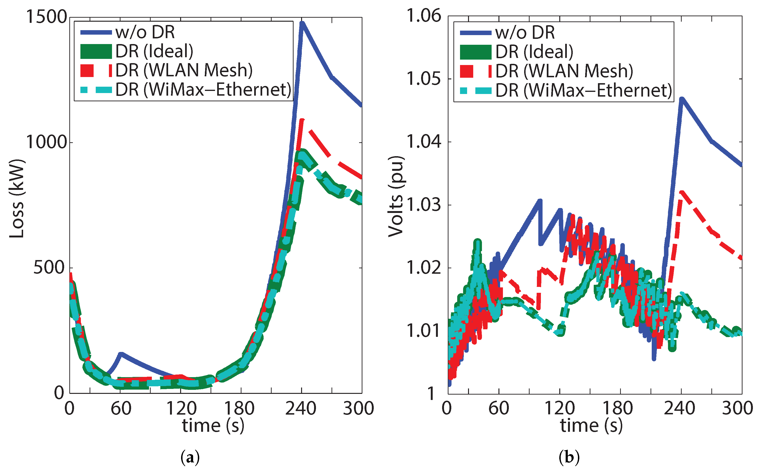
Figure 13.
The CDF of the packet transmission delay.
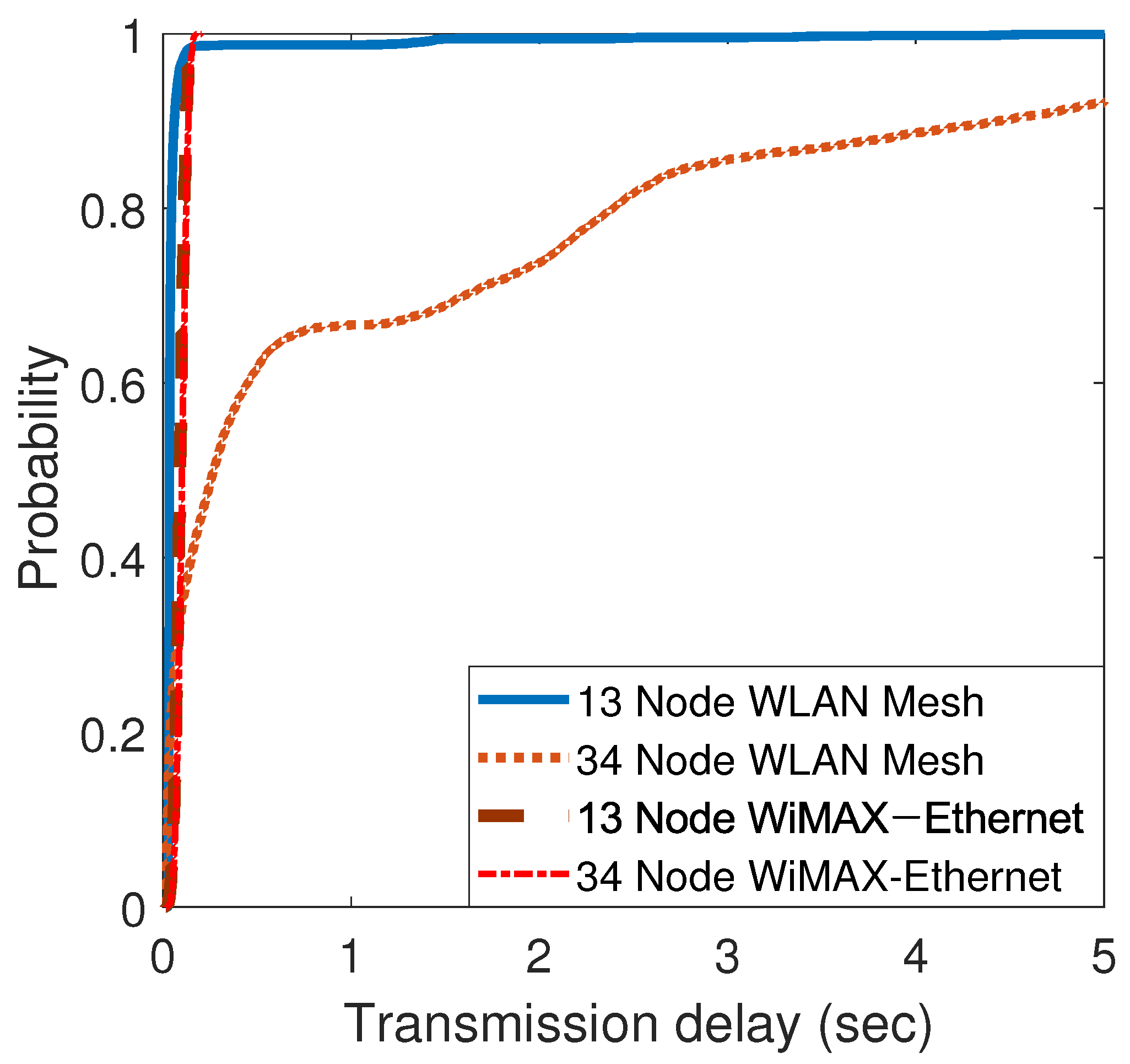
Figure 14.
The usage of memory and cpu of simulation scenarios. (a) Memory usage; (b) CPU usage.

Figure 15.
The simulation time of multiple smart grid systems.


Table 1.
Total cost of each scenario.
| 13 Node System | 34 Node System | |
|---|---|---|
| w/o DR | 679.272 | 362.568 |
| DR | 579.617 | 308.449 |
| Saving | 14.7% | 14.9% |
Table 2.
The power loss and the voltage of 13 Node system.
| Total Power Loss | Voltage Index | |
|---|---|---|
| w/o DR | 33,385 kW | 0.1533 |
| DR (Ideal) | 22,795 kW | 0.0741 |
| DR (WLAN Mesh) | 23,125 kW | 0.0783 |
| DR (WiMax-Ethernet) | 23,094 kW | 0.0825 |
Table 3.
The power loss and the voltage of 34 Node system.
| Total Power Loss | Voltage Index | |
|---|---|---|
| w/o DR | 136,180 kW | 0.4156 |
| DR (Ideal) | 94,545 kW | 0.2686 |
| DR (WLAN Mesh) | 119,340 kW | 0.6101 |
| DR (WiMax-Ethernet) | 95,412 kW | 0.2735 |
Table 4.
Execution time of simulation study.
| 13 Node WLAN Mesh | 34 Node WLAN Mesh | 13 Node WiMax-Ether | 34 Node WiMax-Ether | |
|---|---|---|---|---|
| OPNET execution time | 75.4 s | 568.4 s | 12.7 s | 57.3 s |
| # of OPNET events | 15,520,756 | 136,464,504 | 2,563,603 | 10,880,800 |
| OpenDSS execution time | 6.2 s | 38.7 s | 6.3 s | 43.7 s |
| # of OpenDSS events | 3764 | 16,497 | 3900 | 20,700 |
| Total execution time | 81.6 s | 607.1 s | 19.0 s | 101.0 s |
© 2018 by the authors. Licensee MDPI, Basel, Switzerland. This article is an open access article distributed under the terms and conditions of the Creative Commons Attribution (CC BY) license (http://creativecommons.org/licenses/by/4.0/).
Share and Cite
MDPI and ACS Style
Kim, H.; Kim, K.; Park, S.; Kim, H.; Kim, H. CoSimulating Communication Networks and Electrical System for Performance Evaluation in Smart Grid. Appl. Sci. 2018, 8, 85. https://doi.org/10.3390/app8010085
AMA Style
Kim H, Kim K, Park S, Kim H, Kim H. CoSimulating Communication Networks and Electrical System for Performance Evaluation in Smart Grid. Applied Sciences. 2018; 8(1):85. https://doi.org/10.3390/app8010085
Chicago/Turabian StyleKim, Hwantae, Kangho Kim, Seongjoon Park, Hyunsoon Kim, and Hwangnam Kim. 2018. "CoSimulating Communication Networks and Electrical System for Performance Evaluation in Smart Grid" Applied Sciences 8, no. 1: 85. https://doi.org/10.3390/app8010085
Note that from the first issue of 2016, this journal uses article numbers instead of page numbers. See further details here.