Novel Measurement Method for Determining Mass Characteristics of Pico-Satellites


School of Aeronautics and Astronautics, Zhejiang University, Hangzhou 310027, China
*
Author to whom correspondence should be addressed.
Appl. Sci. 2018, 8(1), 104; https://doi.org/10.3390/app8010104
Submission received: 7 December 2017
/
Revised: 6 January 2018
/
Accepted: 10 January 2018
/
Published: 15 January 2018
(This article belongs to the Section Mechanical Engineering)
Abstract
:The centroid and moment of inertia directly affect the dynamic characteristics of aircraft, and accurate mass characteristic measurements are crucial to adequately control aircraft attitude. This paper proposes a new measurement method for determining aircraft mass characteristics that can improve measurement precision when used in regard to pico-satellites. The measurement system is designed according to the principles of three-point measure and constant torque. The feasibility of the test method of this study for determining the mass characteristics is proved by using a dynamic simulation and an experimental analysis method. Through a number of standard workpiece tests, the deviation of the measurement system and effective compensation methods of the mass characteristics are obtained. The measurement system and compensation methods are applied to measure the mass characteristics of a pico-satellite, which can be detected by only one time clamping. The measurement system proposed herein can effectively improve measurement precision, as it was found that the accuracy of the centroid and the moment of inertia of the pico-satellite are less than 1 mm and 1.5 × 10⁻² kgm2, respectively. The proposed measurement system also has many advantages, such as a simple operation, high efficiency, small volume, and low cost.
1. Introduction
Mass characteristics provide the theoretical basis and the important parameters for aircraft design, flight attitude, and orbit control, and they are also important criteria for evaluating products [1]. The measurement of mass characteristics is widely used in aerospace, weapon systems, precision instruments, and industrial machinery. With continuous global development in the field of aerospace, the measurement of aircraft mass characteristics has gained attention by international scholars. When the centroid and moment of inertia of the aircraft’s high-speed movement cannot be accurately measured, the direction of aircraft flight and attitude will be very difficult to adjust, which can lead to loss of control of the aircraft. Improving the measurement precision of the aircraft mass characteristics has become an inevitable requirement of national science and technology development, and world scholars and research institutions are currently conducting research on the measurement algorithm and methodology of mass characteristics.
Bergman et al. [2] developed an algorithm for the estimation of spacecraft mass characteristics using only torque-producing actuators. This capability enhances the usefulness of an autopilot function that is capable of adapting to changes in the spacecraft’s mass characteristics. Boynton [3] presented a case history of instances where errors in measuring mass properties have occurred, and many of these challenges could have been avoided. Psiaki [4] developed a new algorithm that used on-orbit data to estimate the moment of inertia. The best estimates of the moment of inertia and scale factor in the reaction wheel obtained from the algorithm are better than those from preflight estimates. Qin et al. [5] theoretically presented the characteristics of an inertia measurement system with accelerometers and attitude control algorithm, and the validity of the attitude control algorithm was proved via a simulation and experiment on the ground. Bois et al. [6] presented a derived formula to calculate the moment of inertia using a trifilar suspension system and the measurement system errors were determined via a specific experiment. Dong [7] combined the batch least squares method and the extended Kalman filter to estimate inertia parameters to eliminate the influence of measurement noise on the results. Norman [8] presented a series of estimation schemes based on measurement algorithms to measure the mass characteristics of spacecraft. The validity of the algorithms was proved via comparing simulation and on-orbit data. Zhu [9] experimentally investigated the inertia characteristics measurements for vehicles and proposed an error analysis method. The results show that the method has a high accuracy for measuring the inertia parameters of vehicles. Chashmi [10] proposed a fast and generalized formulation to identify the moment of inertia of a spacecraft. The formulation has a larger scope of application than previous ones in the space industry.
Lee [11] proposed and validated a methodology to estimate the moment of inertia of the Cassini spacecraft, and the method estimated the moments and products of inertia of the spacecraft whenever telemetry data associated with the slewing of the spacecraft by the reaction wheels was available. Peterson [12] described the techniques used to measure mass characteristics for a series of spacecraft. The measured mass characteristics also provided the means for the aerodynamicists to derive the aerodynamic parameters obtained during the flight tests. Ma [13] proposed a novel on-orbit measure method for characteristics of the moment of inertia of spacecraft, while considering both estimation models with a known initial angular momentum and an unknown initial angular momentum. Hou et al. [14] and Tang [15] utilized an improved trifilar pendulum method to measure mass characteristics. Further, they proposed an error evaluation method for the measurement system, and the novel methods were proved by experiments. Hejtmánek et al. [16] presented a test method to determine the moment of inertia of a motor vehicle. A test platform was designed and the measurement error of the test platform was analyzed. Dudarenko et al. [17] presented a novel method to identify the moment of inertia and centroid of a rigid body applied to the work-energy principle. They proposed methods to process data and estimate system error. Zhang [18] designed a method to estimate the inertia for space debris. This method consisted of three phases: coarse and precise estimate of mass and estimate of the moments of inertia. Shakoori et al. [19] investigated three common measurement methods of moments of inertia and presented a new method to evaluate measurement error. The results of the analysis show that the bifilar torsional pendulum method has a lower error than other methods. Mondal [20] designed and optimized a mass property measurement system; therein, the air bearing and flexure applied to the measurement system greatly improve the measurement accuracy. Zhai [21] presented a new method for designing the optimal excitation of identifying inertia parameters, and the simulation results showed that the calculated optimal excitation has a good performance index and can produce accurate identification results even when some perturbations are considered. Fakhari [22] theoretically and experimentally investigated the effects of disturbances on the inertia measurement system. The disturbances could be eliminated via some solutions to improve measurement accuracy.
However, the above measurement algorithm and methodology mainly involve common measurement procedures for mass characteristics, and the measurement of centroid position can be achieved via three point weighting, suspension, and balancing method. There are three main safe and popular methods to measure the moment of inertia: period of free oscillation, torque, and pendulums methods [14,15,23]. However, there are several drawbacks to implementing these methods. They must use different machines to measure the centroid and moment of inertia, and in addition, the test body must be clamped many times and different fixture tools must be used when measuring the mass characteristics of different directions, and the high precision sensors must be used and a large number of test data need to be collected and processed; hence, those measurement methods are of high risk to the product, expensive, and time consuming.
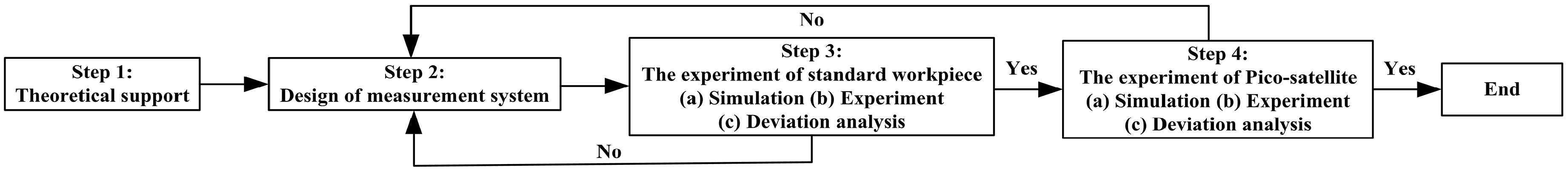
Hence, this paper proposes a new measurement method for determining mass characteristics, and the feasibility of this test method is proved by using a dynamic simulation and an experimental analysis method. A summary of the paper is shown in Figure 1. The measurement system for determination of the mass characteristics is designed and developed, and through a number of standard workpiece tests, the deviation of the measurement system and effective compensation methods of the mass characteristics are obtained. The measurement system and compensation methods are applied to measure the mass characteristics of a pico-satellite. In addition, the measurement system not only improves the accuracy of the centroid and moment of inertia determination of the pico-satellite, but it also has several advantages, such as a simple operation, high efficiency, small volume, and low cost.
2. The Measurement Principle of Mass Characteristic
2.1. Principles of Measurement of Mass Characteristics
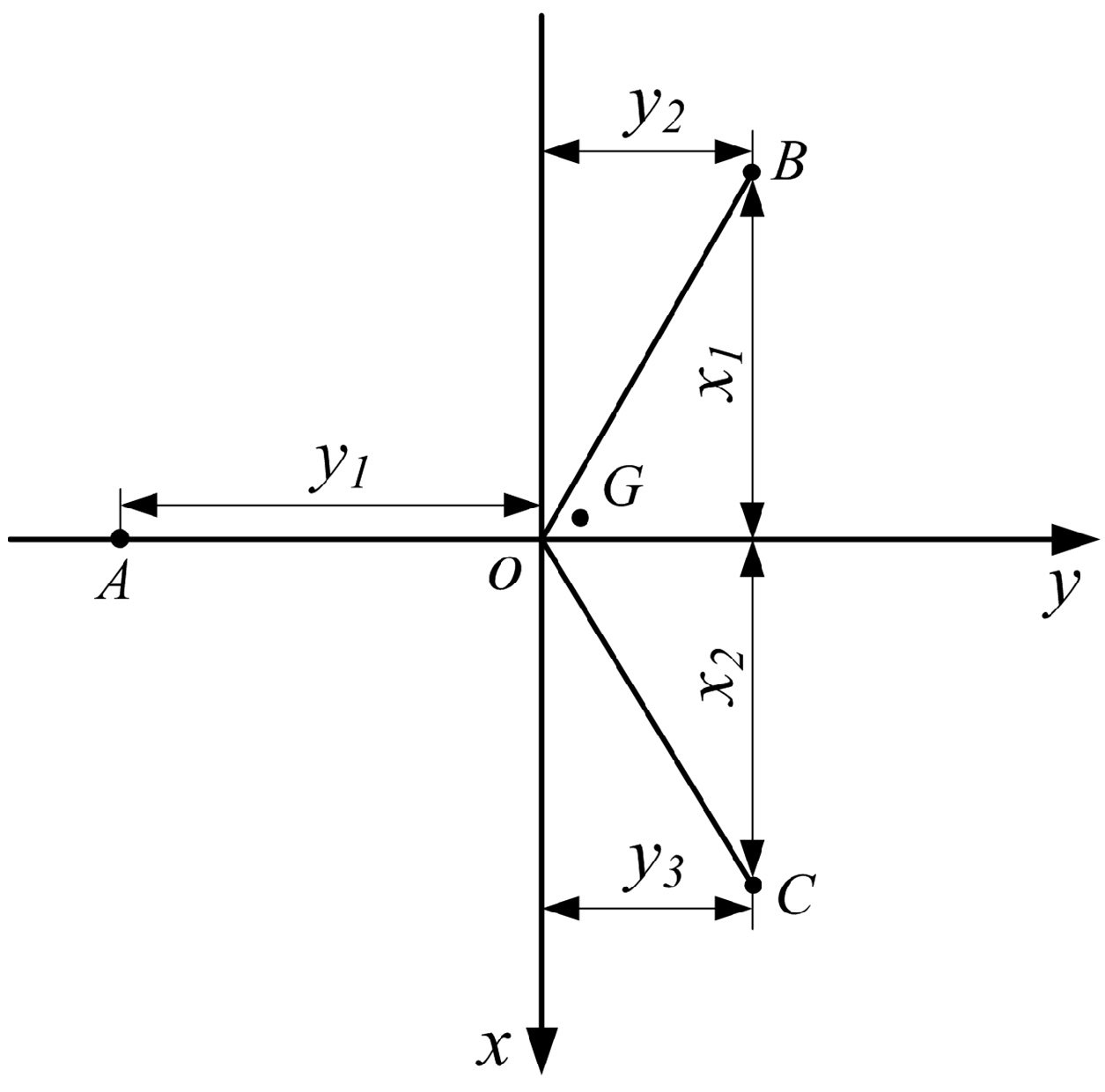
The test for determining the centroid is based on the principle of three-point measurement [24]. First, the measurement system uses a coordinate system (), which is located at the center of rotation, as shown in Figure 2. Three weighing sensors, which are identified as , , and ( mm), are located in the plane with an angle of 120° between them. Hence, the mass of the pico-satellite can be obtained:
where, , , and represent the measurement values of the total mass of the fixture tools and worktable of the three weighing sensors, , , and , respectively. , , and represent the measurement values of the total mass of the fixture tools, worktable, and pico-satellite of the three weighing sensors , , and , respectively. , , and are the satellite weights which are calculated according to , , , , , and in , , and three points, respectively. is the total mass of the pico-satellite.
According to the principle of moments [9], when the moment is considered from the -axis, the centroid of the pico-satellite in the -direction can be expressed as:
where , , and are the distances from the -axis, respectively.
When the moment is taken from the -axis, the centroid of the pico-satellite in the -direction can be expressed as:
where and are the distances from the -axis, respectively.
After the measurement system rotates by a 90° angle, , the centroid of the pico-satellite in the -direction can be obtained.
2.2. Test Principle for Determining the Moment of Inertia
According to the angular momentum theorem [25], the time derivative of the angular momentum of the particle system at any fixed point is equal to the vector sum of the moments of the external forces acting on that point . This can be expressed as:
where is the vector sum of the external moments of particle system, is the angular momentum, and is the time.
Angular momentum can be expressed as:
where is the moment of inertia, and is the angular velocity.
According to Equations (7) and (8), can be expressed as:
where is the angular acceleration.
When the different particle systems are identical to the external moment () of the same fixed point , can be expressed as:
When integration is used on both sides of Equation (10), it can be expressed as:
According to Equation (11), the final expression is:
In the actual measurement procedure, the external moment of the measurement system contains the output torque () of the motor, the friction torque () produced by the friction force of the reduction drive and bearings, and the air resistance torque () generated by the air. The sum of the external moments () can be expressed as:
Because and , the total moment of the actual measurement system is approximately equal to .
The moment of inertia of the fixture tools and worktable is , the motor starting acceleration time is , the rated angular velocity is , and the angular velocity at time () is . Hence the relationship of the angular velocity () and the start time of () can be expressed as:
Assuming the moment of inertia of the pico-satellite in the direction of rotation is , when the pico-satellite is equipped with the measurement system, the motor starting time is , the rated angular velocity is , and the angular velocity at time () is . Then, the relationship of the angular velocity () and the start time of can be expressed as:
When Equations (14) and (15) are in the same time (), the angular velocities of Equations (14) and (15) are and , respectively.
According to Equation (12), it can be expressed as:
Then, according to Equation (16), the moment of inertia of the pico-satellite () in the direction of rotation can be expressed as:
After the measurement system rotates 90°, the moments of inertia of the pico-satellite ( and ) in the other two directions can also be obtained.
3. Measurement System to Determine Mass Characteristics
The structural diagram of the mass characteristic measurement system is shown in Figure 3. The measurement system is mainly composed of a rack, servo motor (parameters are listed in Table 1), speed reducer (parameters are listed in Table 2), shaft coupling, bearings, spindle, worktable, guide rail, slider block, weighing sensors (parameters are listed in Table 3), angular velocity sensor (parameters are listed in Table 4), lifting platform, and fixture tools.
The lifting platform moves up and down to obtain data from the three weighing sensors, and the centroid of the pico-satellite can then be calculated.
The four screws are connected to the main shaft and worktable, and the servo motor drives the worktable through a speed reducer and the main shaft. The angular velocity sensor transmits the data to the computer, and the different positions and the states of the angular velocity can be obtained. Then, the moments of inertia of the pico-satellite can be calculated.
The design requirements for the measurement deviation of the mass characteristic measurement system are listed in Table 5.
4. Simulation and Experiment of the Standard Workpiece
To obtain the measurement accuracy of the measurement system and optimize the measurement results, a standard workpiece is used to perform the test, and the experimental data of the standard workpiece can be obtained. The standard workpiece is a hollow-walled cube with a uniform thickness of 8 mm, dimensions of mm3, and a total weight of 26.647 kg. The thickness of the worktable is 10 mm, and the position of the centroid of the standard workpiece is . The positional relationship between the standard workpiece and the mass characteristic measurement system is shown in Figure 4.
Solidworks was utilized to build the 3D standard workpiece model, which was modeled using the real mass attributes to determine the theoretical mass characteristic parameters. The theoretical parameters of the standard workpiece are listed in Table 6. The moment of inertia of the standard workpiece with respect to the -axis of the origin coordinate system is ; when the origin coordinate system is in the position of the centroid, the moment of inertia of the standard workpiece is .
4.1. Simulation Measurement of the Centroid of the Standard Workpiece
The 3D standard workpiece model was imported into Adams (Mechanical Dynamics Inc., Los Angeles, CA, USA, 2013), a multibody dynamics simulation solution software, to simulate the centroid and moment of inertia of the standard workpiece with the gravitational acceleration set to m/s2. The simulation data of the standard workpiece can be obtained at three points (, , and ), and the simulation measurement results are shown in Table 7.
4.2. Experimental Measurement of the Centroid of the Standard Workpiece
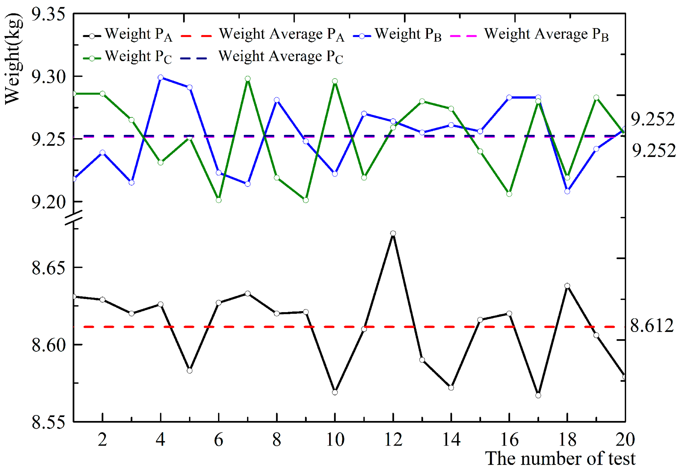
The moment of inertia of the standard workpiece was measured 20 times via the measurement system to reduce the changes in the results of the centroid determination caused by sensor deviation. The experimental results are shown in Figure 5, and the three curves represent the measurement values of sensors , , and , respectively. According to Equation (21), we can obtain the average values from the , , and sensors, which are 8.612 kg, 9.252 kg, and 9.252 kg, respectively, and the average values are used as the final experimental data. The comparison of the centroid of the standard workpiece between the simulation and experimental results is shown in Table 8.
It can be determined from Table 8 that there are deviations between the experimental and theoretical results in the actual measurement. The main factors that cause these deviations are parts processing deviation, assembly deviation, and weighing sensor deviation. Table 3 shows that the deviation of the weighing sensor is ±0.05%. It is assumed that the deviations are mainly affected by the weighing sensors in the measurement system, and the maximum deviation of the centroid in the -axis direction can be expressed as:
When kg, mm, and hence mm, and mm. Table 8 shows that the measurement accuracy in the -axis direction meets the design requirements. According to the principle of moments, the value of the weighing sensors increases as the three points approach the coordinate origin in the direction of the -axis. Table 8 indicates that the experimental coordinates () are mm and mm. The mass of each millimeter in the OA, OB, and OC directions is kg/mm, and therefore, the positions of the actual weighing sensors in the -axis direction are mm and mm, respectively. After compensation, the actual position of the centroid is (0, −0.09), and the deviations are , , and , respectively. The results show that the deviations meet the requirements of precision.
4.3. Simulation Measurement of the Moment of Inertia of the Standard Workpiece
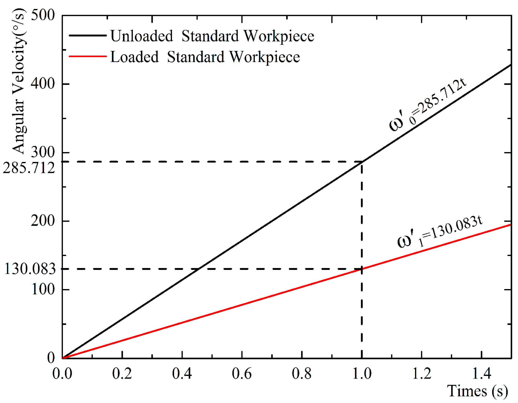
The 3D standard workpiece model was imported into Adams, and the gravitational acceleration and torque were set to m/s2 and Nm, respectively. The simulation values of the moment of inertia of the standard workpiece are shown in Figure 6. The equation represents the relationship between the angular velocity and time when the standard workpiece is not loaded. The equation is the relationship between the angular velocity and time when the standard workpiece is loaded. When is 1 s, the corresponding angular velocities ( and ) can be obtained. When the standard workpiece is not loaded, the moment of inertia of the measurement system is . According to Equation (17), the moment of inertia of the standard workpiece () can be obtained. The simulation results of the standard workpiece are summarized in Table 9.
4.4. Experimental Measurement of the Moment of Inertia of the Standard Workpiece
The moment of inertia of the standard workpiece was measured 100 times via the measurement system. In the actual measurements, the output torque of the servo motor was not an ideal constant. In reality, the output torque experienced certain fluctuations. The angular velocity when the servo motor started exhibited a great deviation. Therefore, it could collect the angular velocity and time of acceleration period of the servo motor to fit the average angular acceleration of motor , which can be expressed as:
The angular acceleration results obtained from the experimental measurements are shown in Figure 7. The two curves are the angular acceleration values measured 100 times when the measurement system is both not loaded and loaded with the standard workpiece, and according to Equation (24), the average values of these angular accelerations are 285.712°/s and 130.083°/s, respectively.
According to the average angular acceleration values, the relationship between the angular velocity and the motor starting time is shown in Figure 8. and demonstrate the relationship between the angular velocity and time when the standard workpiece is both not loaded and loaded, respectively. According to Equations (14)–(17), when is 1 s, the corresponding angular velocities of and can be obtained, and the moment of inertia of the standard workpiece () can also be obtained.
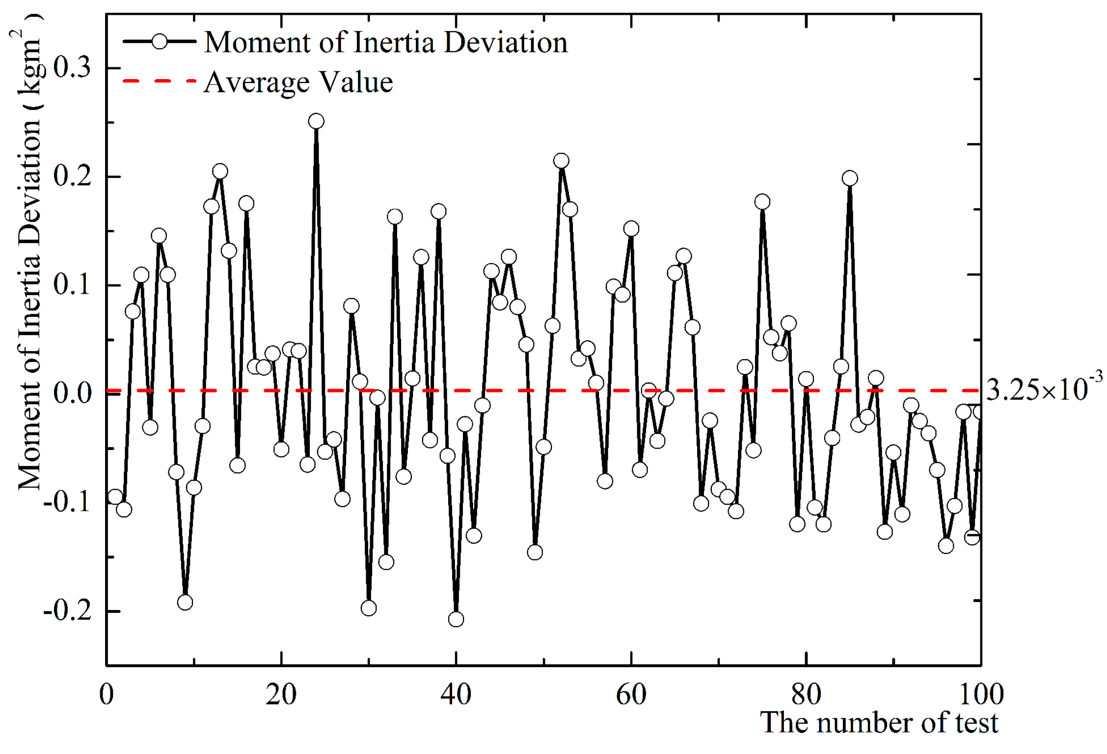
The deviation and comparison of the moments of inertia between the experimental and the theoretical values is shown in Figure 9 and Table 10. We know that the maximum value of the deviation is 4.105 × 10⁻² kgm2 and the minimum value of the deviation is −4.241 × 10⁻² kgm2 from Figure 9. The () in the table is the difference between the experimental and theoretical values of the moment of inertia.
Because the motor output torque exhibits fluctuation during the motor starting process, the angular acceleration changes with this change in the output torque. This affects the moment of inertia measurements, and this is confirmed in Figure 7. The accuracy of measurement results can be improved through using the method of angular acceleration, and this is confirmed in Figure 9.
5. Measurement of Mass Characteristics of the Pico-Satellite
The measurement characteristics of the measurement system can be obtained from the comparison between the standard workpiece simulation and the experimental data, and it can improve the accuracy of determining the mass characteristics of the pico-satellite. According to the layout of the pico-satellite, the theoretical mass characteristics can be obtained. To compare the pico-satellite experimental data and the theoretical values, the pico-satellite model was built using Solidworks and was given the real mass attributes to obtain the theoretical parameters of the mass characteristics. The pico-satellite parameters are listed in Table 11.
The measurement system was used to measure the mass characteristics of the pico-satellite, and the pico-satellite was equipped in different measuring states, as shown in Figure 10. In the vertical state, the origin coordinates of the pico-satellite coincide with the origin coordinates of the measurement system, as shown in Figure 10a. The coordinate systems of the pico-satellite horizontal position- and horizontal position- are shown in Figure 10b,c, respectively.
5.1. Determination of Centroid of Pico-Satellite
The measurement system measures the mass of the three points five times when the satellite is not loaded, and the average values are used for the final experimental results, as shown in Table 12. The measurement system also measures the mass of the three points five times when the satellite is loaded. Hence, the three-point mass of the pico-satellite in three states of Figure 10 was obtained, and the average values were used for the final experimental results. As noted in Section 4.2, mm and mm, according to Equations (5) and (6), and the experimental values of the pico-satellite in different states can be obtained. The comparison of centroid values between the experimental and theoretical results of the pico-satellite is shown in Table 13.
Table 13 shows that the actual deviation of the pico-satellite centroid is 0.766 mm, 1.271 mm, and 0.208 mm, respectively. These results satisfy the design requirements of the measurement system.
5.2. Measurement of the Moment of Inertia of the Pico-Satellite
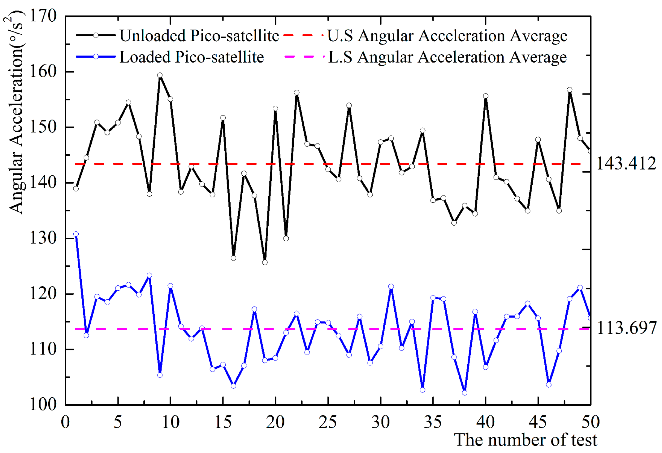
The measurement system measured the moment of inertia of the pico-satellite 50 times in different positions and states, and the experimental values obtained from the angular acceleration results are shown in Figure 11, Figure 12 and Figure 13. The curves in the figures represent the experimental values of the angular acceleration without the pico-satellite and with the pico-satellite, respectively. The dashed lines represent the averages of the angular acceleration.
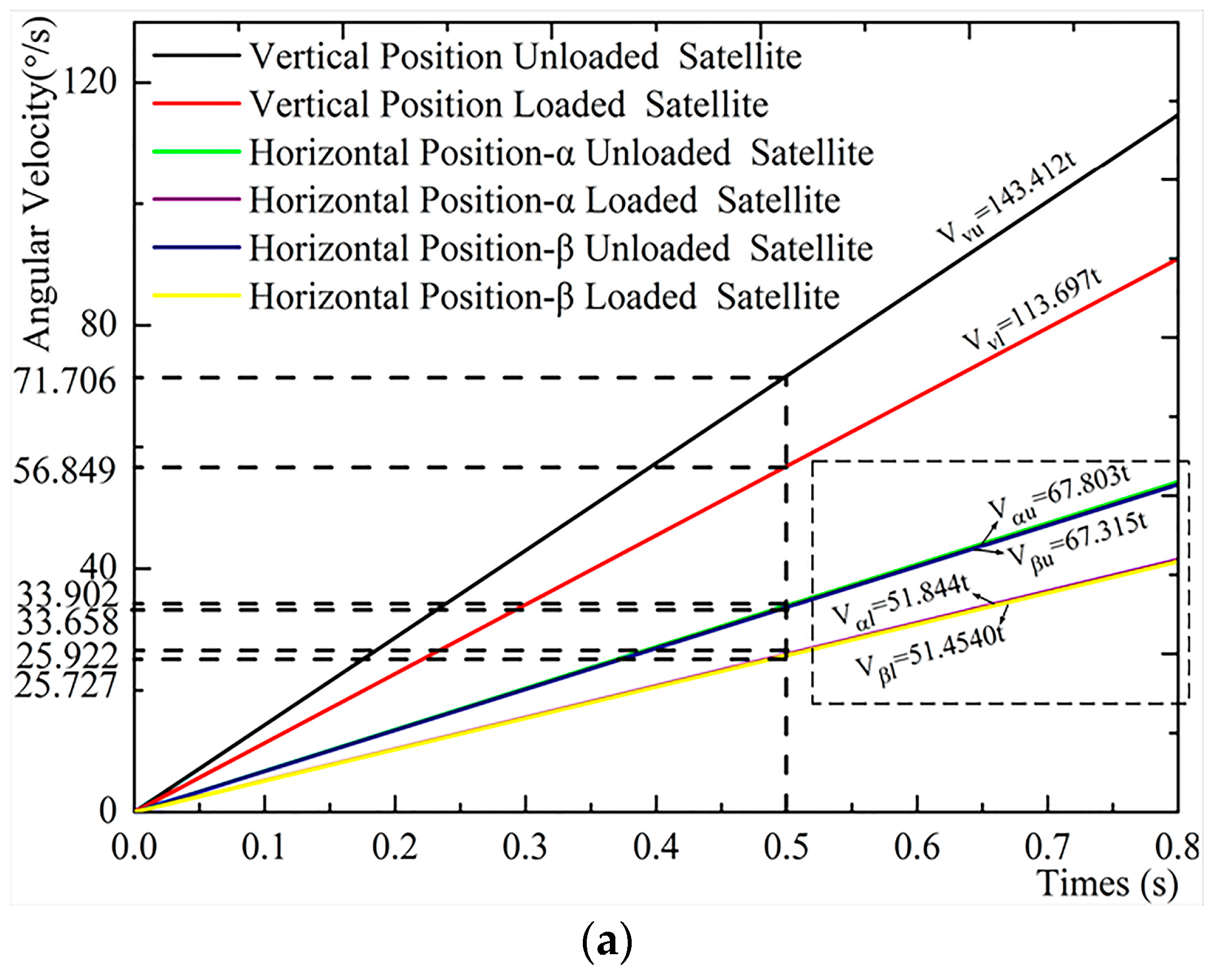
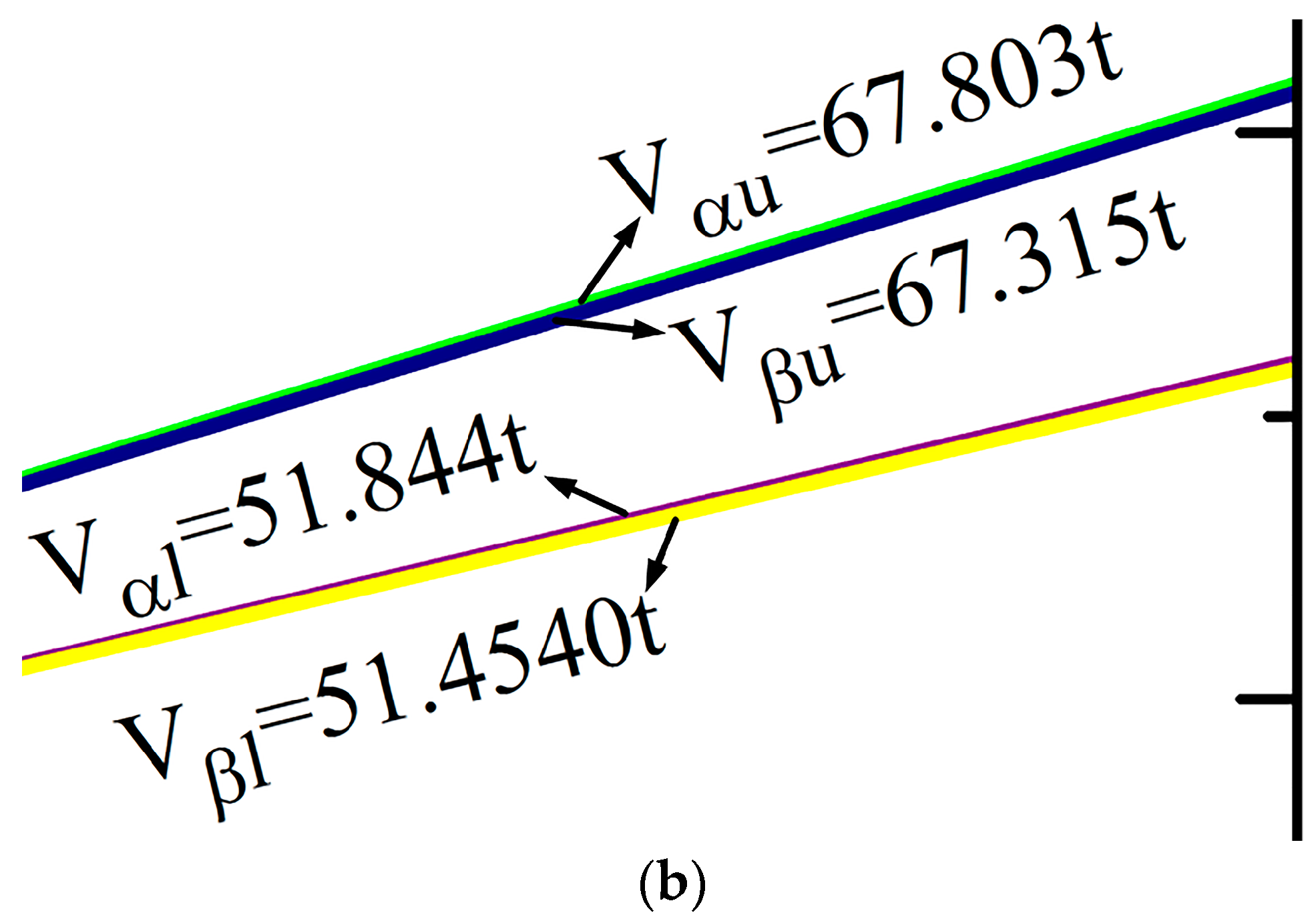
The relationship between the angular velocity and the motor starting time can be obtained based on the average values of the angular acceleration, as shown in Figure 14. In Figure 14, is the relationship between the angular velocity and time when the pico-satellite is not loaded in the vertical position. is the relationship between the angular velocity and time when the pico-satellite is loaded in the vertical position. is the relationship between the angular velocity and time when the pico-satellite is not loaded in the horizontal position-. is the relationship between the angular velocity and time when the pico-satellite is loaded in the horizontal position-. is the relationship between the angular velocity and time when the pico-satellite is not loaded in the horizontal position-. is the relationship between the angular velocity and time when the pico-satellite is loaded in the horizontal position-.
According to Equations (14)–(17), when is 0.5 s, the corresponding angular velocity values of and can be obtained. The moment of inertia of the measurement system is when the pico-satellite is not loaded, thus allowing us to determine the moment of inertia of the experimental value (). According to Equations (18)–(20), the moment of inertia of the pico-satellite can be obtained when the coordinate origin is located at the center of mass. The comparison of the moment of inertia between the experimental and theoretical results of the pico-satellite is shown in Table 14.
Table 14 also shows that the moment of inertia deviations of the pico-satellite are 1.7 × 10⁻³ kgm2, 1.49 × 10⁻² kgm2, and 1.37 × 10⁻² kgm2, respectively. The measurement results can also satisfy the design requirements of the measurement system.
6. Discussion
The measurement system deviations for determining the mass characteristics of the pico-satellite can be caused by several reasons. First, there are deviations between the 3D design, actual machining, and assembly of the measurement system. Second, there are deviations between the 3D design, actual machining, and assembly of the standard workpiece, work fixture, and pico-satellite that can affect the position of the centroid and moment of inertia. Third, the weighing and angular velocity sensors have a certain measurement deviation, which can lead to deviation in the centroid and moment of inertia. Moreover, the measurement system has friction resistance and air resistance, and the torque of the motor has periodic deviation, which could lead to the deviation of the angular velocity. Additionally, the horizontal tilt of the system can also lead to deviations of the centroid and moment of inertia.
The measurement system has application limits, and the motor torque parameters, weighing sensor parameters, experimental safety, and accuracy should be considered when determining these application limits. The weight range of the measurement object is 10–50 kg; the deviation range of the centroid is 0–250 mm; and the range of the moment of inertia is 0.08–1 kgm2. The measurement time of the centroid is less than 15 min, and the measurement time of the moment of inertia is less than 20 min, which is a small amount of time when considering the applicability of the measurement system. In addition, the deviation of the centroid and moment of inertia is less than 2.5 mm, 1.5 mm, 20 kgm2, and 0.6 kgm2 in the literature [9,15], respectively, and their accuracy of measurement is inferior to our measurement system. The cost of the measurement system is approximately $50,000 in the literature [25], and the assembly and test process are complicated and time consuming. Hence the mass characteristic measurement system developed herein has many benefits, such as its low cost (approximately $3000), simple processing and assembly, and easy operation.
7. Conclusions
(1) A measurement system for determining mass characteristics is developed based on the three-point measurement method and the constant torque measurement principle, and it can greatly improve the accuracy of the pico-satellite test, reduce the cost, and reduce the measurement time.
(2) The centroid and moment of inertia of the standard workpiece are measured via a comparison between the simulation and the experiment. The cause of the deviations is analyzed, and the error of the measurement is compensated. The deviation of the centroid and moment of inertia are 0.041 mm and 1.6 × 10⁻³ kgm2, respectively. The measurement results can satisfy the measurement design requirements.
(3) The measurement system was applied to measure the centroid and moment of inertia of the pico-satellite. The measurement results show that the centroid deviation is less than 1 mm, and the moment of inertia deviation is less than 1.5 × 10⁻² kgm2. The measurement results show that the precision of the measurement system can satisfy the measurement design requirements.
Author Contributions
Lai Teng made substantial contributions to design of the work, designed the experiment, collected data and implemented analysis, and drafted the work. Hao Yang made substantial contributions to collected data and implemented analysis, and drafted the work. Zhonghe Jin made substantial contributions to the conception of the work, and revised it critically for important intellectual content.
Conflicts of Interest
The authors declare no conflict of interest.
References
- Bacaro, M.; Cianetti, F.; Alvino, A. Device for measuring the inertia properties of space payloads. Mech. Mach. Theory 2014, 74, 134–153. [Google Scholar] [CrossRef]
- Bergmann, E.V.; Dzielski, J. Spacecraft mass property identification with torque generating control. J. Guid. Control Dyn. 1990, 13, 99–103. [Google Scholar] [CrossRef]
- Boynton, R. Mass properties measurement errors which could have been easily avoided. In Proceedings of the 58th Annual Conference of the Society of Allied Weight Engineers, San Jose, CA, USA, 24–26 May 1999. [Google Scholar]
- Psiaki, M.L. Estimation of a Spacecraft’s attitude dynamics parameters by using flight data. J. Guid. Control Dyn. 2005, 28, 594–603. [Google Scholar] [CrossRef]
- Qin, L.; Zhang, W.; Zhang, H.; Xu, W. Attitude measurement system based on micro-silicon accelerometer array. Chaos Solitons Fractals 2006, 29, 141–147. [Google Scholar] [CrossRef]
- Bois, J.L.D.; Lieven, N.A.; Adhikari, S. Error analysis in trifilar inertia measurements. Exp. Mech. 2009, 49, 533–540. [Google Scholar] [CrossRef]
- Dong, H.K.; Yang, S.; Cheon, D.I.; Lee, S.; Oh, H.S. Combined estimation method for inertia properties of STSAT-3. J. Mech. Sci. Technol. 2010, 24, 1737–1741. [Google Scholar]
- Norman, M.C.; Peck, M.A.; O’Shaughnessy, D.J. In-orbit estimation of inertia and momentum-actuator alignment parameters. J. Guid. Control Dyn. 2011, 34, 1798–1814. [Google Scholar] [CrossRef]
- Zhu, T.; Li, F. Experimental investigation and performance analysis of inertia properties measurement for heavy truck cab. Adv. Mech. Eng. 2015, 7. [Google Scholar] [CrossRef]
- Chashmi, S.Y.N.; Malaek, S.M. Fast estimation of space-robots inertia parameters: Amodular mathematical formulation. Acta Astronaut. 2016, 127, 283–295. [Google Scholar] [CrossRef]
- Lee, A.Y.; Wertz, J.A. In-Flight estimation of the Cassini Spacecraft’s inertia tensor. J. Spacecr. Rocket. 2002, 39, 153–154. [Google Scholar] [CrossRef]
- Peterson, W.L. Mass properties measurement in the X-38 project. In Proceedings of the 63rd Annual Conference of the Society of Allied Weight Engineers, Newport Beach, CA, USA, 17–19 May 2004. [Google Scholar]
- Ma, O.; Dang, H.; Pham, K. On-orbit identification of inertia properties of spacecraft using a robotic arm. J. Guid. Control Dyn. 2008, 31, 1761–1771. [Google Scholar] [CrossRef]
- Hou, Z.C.; Lu, Y.N.; Lao, Y.X.; Liu, D. A new trifilar pendulum approach to identify all inertia parameters of a rigid body or assembly. Mech. Mach. Theory 2009, 44, 1270–1280. [Google Scholar] [CrossRef]
- Tang, L.; Shangguan, W.B. An improved pendulum method for the determination of the center of gravity and inertia tensor for irregular-shaped bodies. Measurement 2011, 44, 1849–1859. [Google Scholar] [CrossRef]
- Hejtmánek, P.; Blatˇák, O.; Kucˇera, P.; Porteš, P.; Vancˇura, J. Measuring the yaw moment of inertia of a vehicle. J. Middle Eur. Constr. Des. Cars 2013, 11, 16–22. [Google Scholar] [CrossRef]
- Dudarenko, N.; Melnikov, V.; Melnikov, G. A method for inertia tensors and centres of masses identification on symmetric precessions. In Proceedings of the 6th International Congress on Ultra Modern Telecommunications and Control Systems and Workshops (ICUMT), St. Petersburg, Russia, 6–8 October 2014. [Google Scholar]
- Zhang, F.; Sharf, I.; Misra, A.; Huang, P.F. On-line estimation of inertia parameters of space debris for its tether-assisted removal. Acta Astronaut. 2015, 107, 150–162. [Google Scholar] [CrossRef]
- Shakoori, A.; Betin, A.V.; Betin, D.A. Comparison of three methods to determine the inertial properties of free-flying dynamically similar models. J. Eng. Sci. Technol. 2016, 11, 1360–1372. [Google Scholar]
- Mondal, N.; Acharyya, S.; Saha, R.; Sanyal, D.; Majumdar, K. Optimum design of mounting components of a mass property measurement system. Measurement 2016, 78, 309–321. [Google Scholar] [CrossRef]
- Zhai, K.; Wang, T.S.; Meng, D.B. Optimal excitation design for identifying inertia parameters of spacecraft. Acta Astronaut. 2017, 140, 370–379. [Google Scholar] [CrossRef]
- Fakhari, V.; Shokrollahi, S. A theoretical and experimental disturbance analysis in a product of inertia measurement system. Measurement 2017, 107, 142–152. [Google Scholar] [CrossRef]
- Brancati, R.; Russo, R.; Savino, S. Method and equipment for inertia parameter identification. Mech. Syst. Signal Process. 2010, 24, 29–40. [Google Scholar] [CrossRef]
- Fu, Y.X.; Jiang, W.S.; Qin, X.S.; Tan, X.Q. Key techniques for the integration of mass, mass and moment of inertia. Machinery 2014, 52, 60–63. [Google Scholar]
- Chen, S.L. The angular momentum theorem for the instantaneous axis. J. Cent. China Norm. Univ. 1988, 20, 135–138. [Google Scholar]
- Abdulghany, A.R. Generalization of parallel axis theorem for rotational inertia. Am. J. Phys. 2017, 85, 791–795. [Google Scholar] [CrossRef]
Figure 1.
A summary of the paper.

Figure 2.
Measurement coordinate system of the centroid.

Figure 3.
Pico-satellite schematic diagram (a) vertical position; (b) horizontal position.
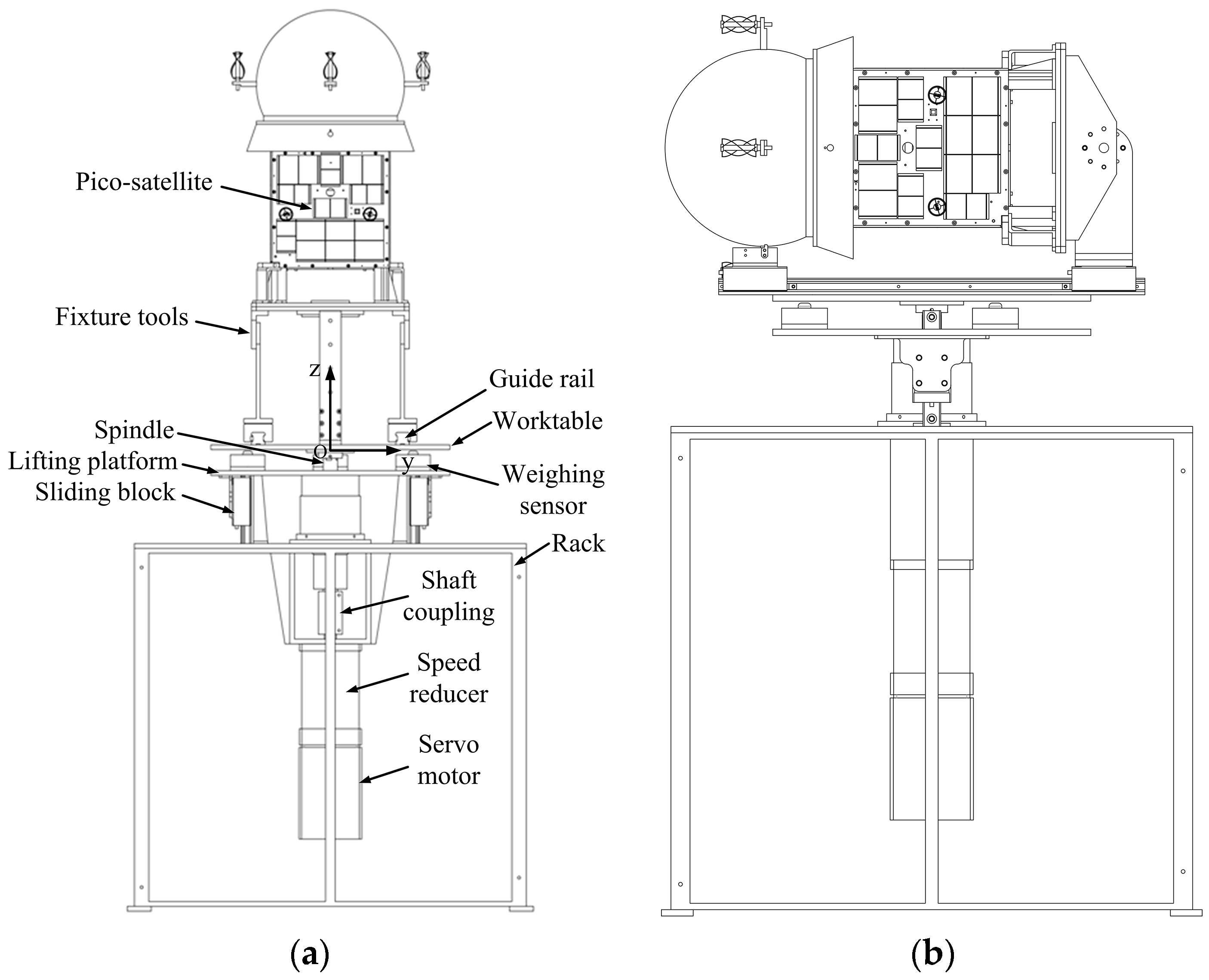
Figure 4.
The position relationship between the standard workpiece and mass measurement system (a) front view; (b) side view.
Figure 4.
The position relationship between the standard workpiece and mass measurement system (a) front view; (b) side view.
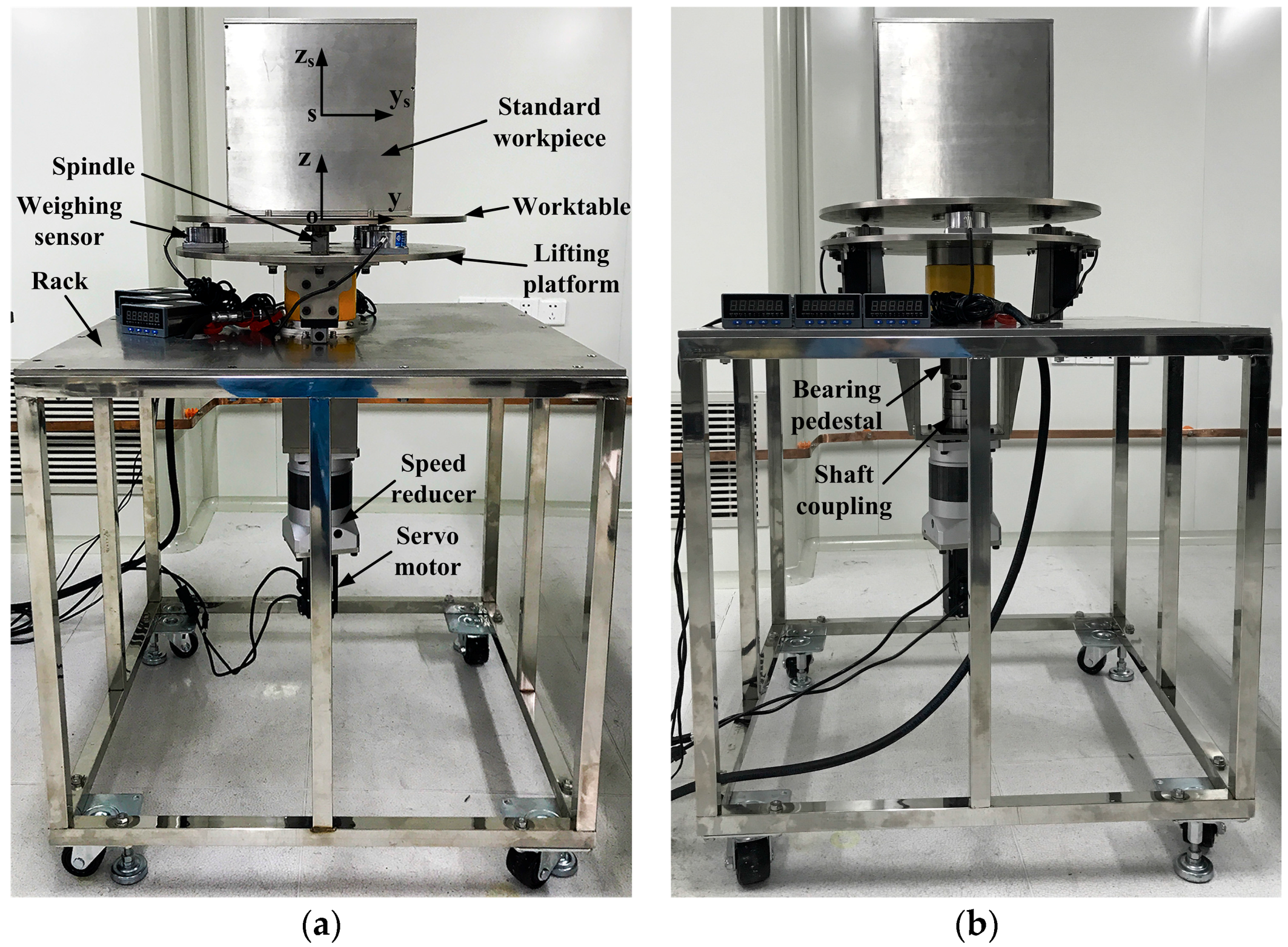
Figure 5.
Standard workpiece mass data at three points.

Figure 6.
The relationship between the angular velocity and time of standard workpiece in different states.
Figure 6.
The relationship between the angular velocity and time of standard workpiece in different states.
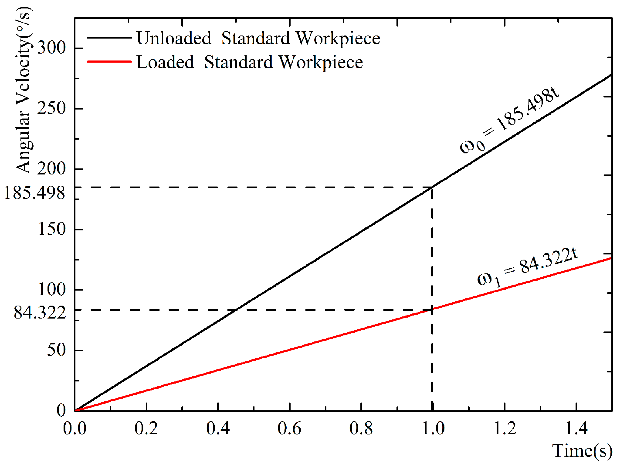
Figure 7.
Angular acceleration in different states.
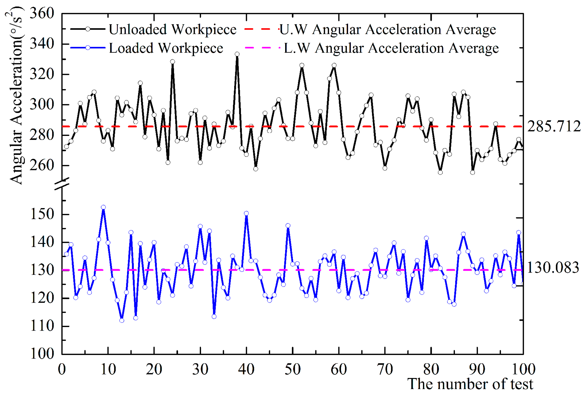
Figure 8.
The relationship between angular velocity and time in different states.

Figure 9.
The moment of inertia difference of the workpiece.

Figure 10.
Different measuring states (a) pico-satellite vertical position; (b) pico-satellite horizontal position-; (c) pico-satellite horizontal position-.
Figure 10.
Different measuring states (a) pico-satellite vertical position; (b) pico-satellite horizontal position-; (c) pico-satellite horizontal position-.
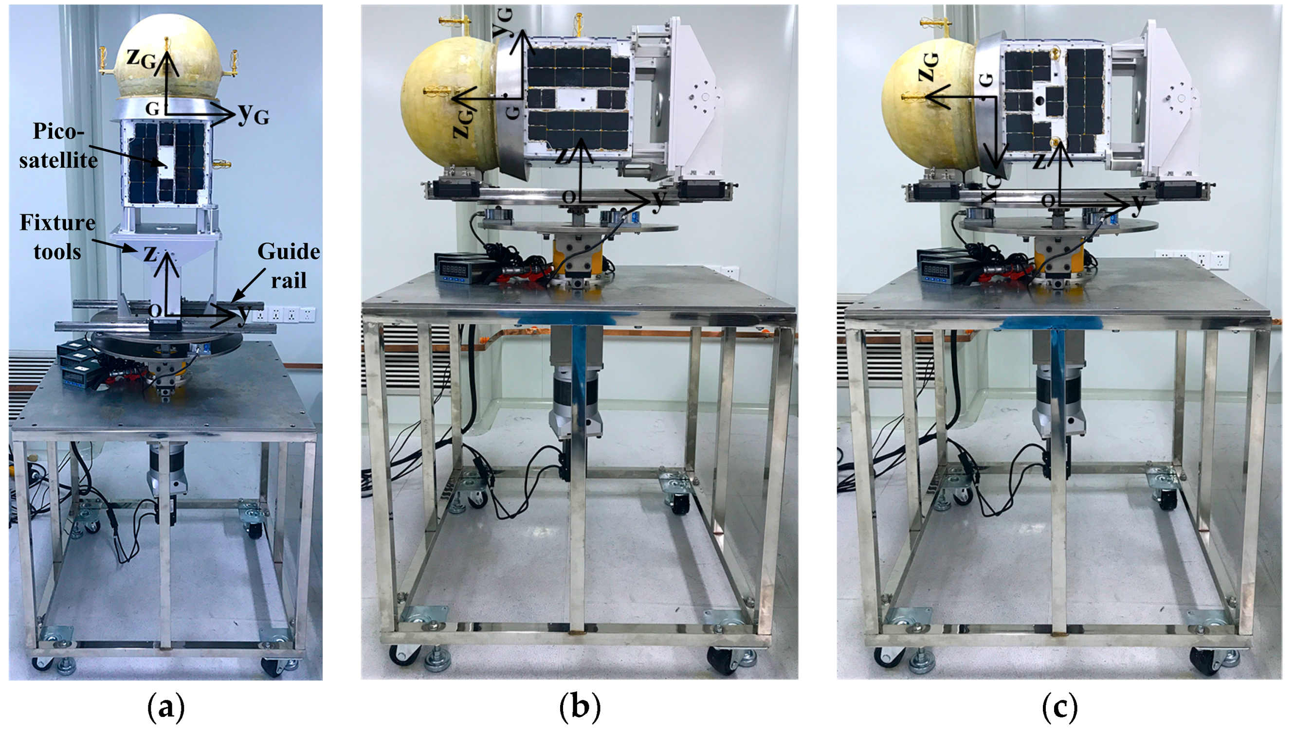
Figure 11.
Angular acceleration in different states at a vertical position.

Figure 12.
Angular acceleration in different states at horizontal position-.
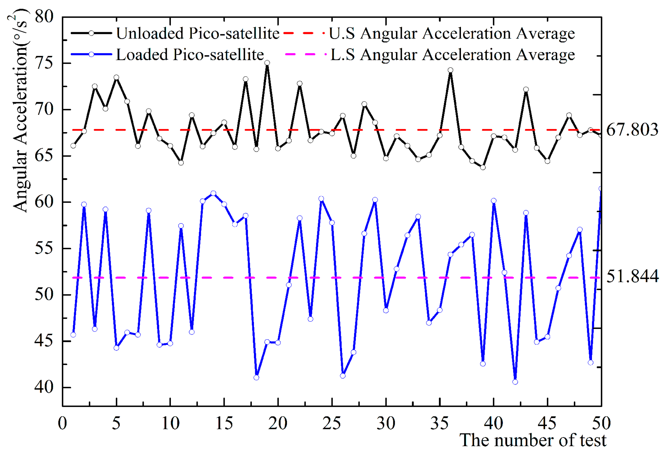
Figure 13.
Angular acceleration in different states at horizontal position-.
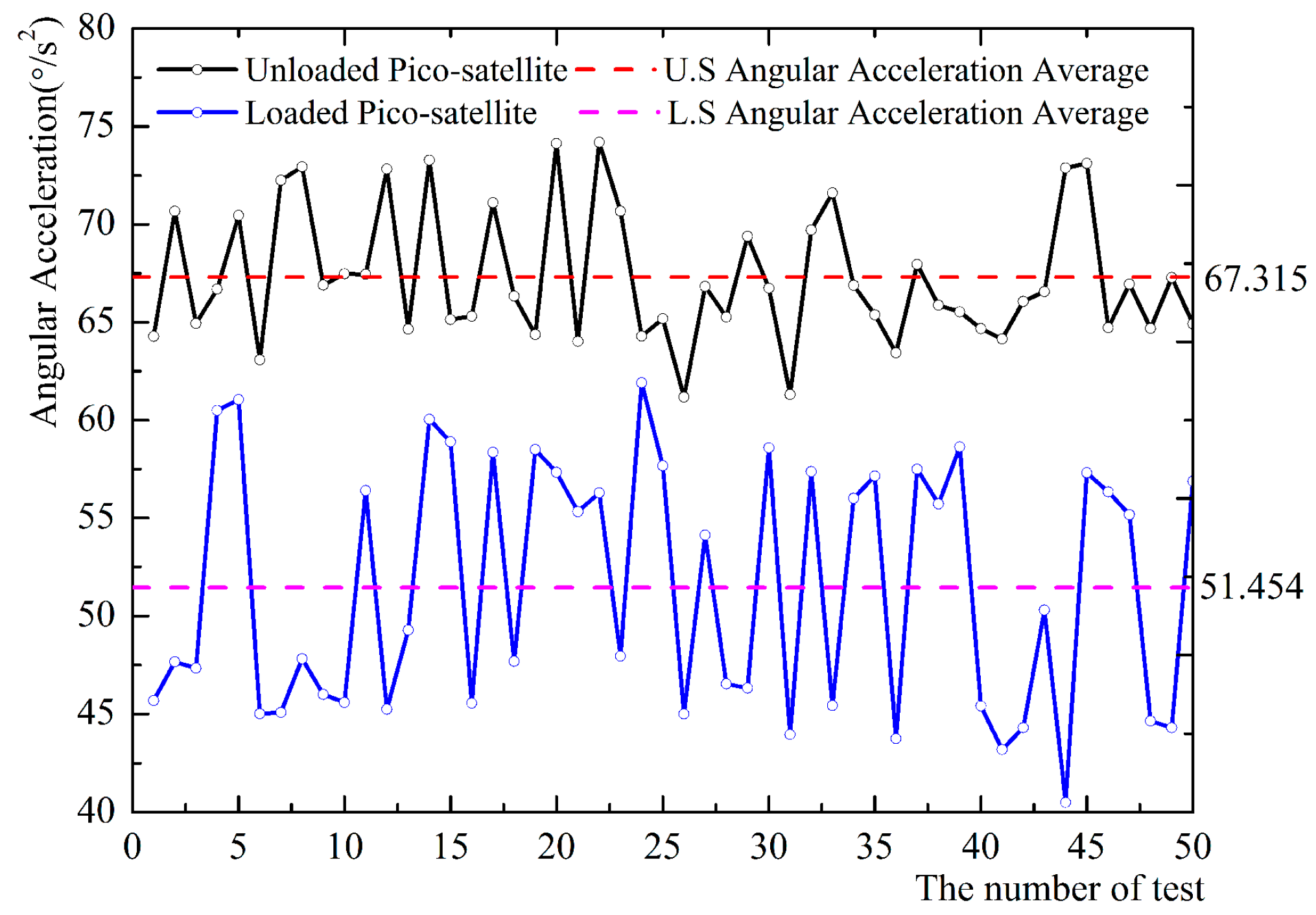
Figure 14.
(a) The relationship between angular velocity and time in different states; (b) the partial enlarged detail in the dash dot frame.
Figure 14.
(a) The relationship between angular velocity and time in different states; (b) the partial enlarged detail in the dash dot frame.


Table 1.
The main parameters of the servo motor.
| Motor Model | Rated Power (KM) | Rated Speed (rpm) | Rated Torque (Nm) | Peak Torque (Nm) |
|---|---|---|---|---|
| LCMT-04L02NB-60M01330B | 0.4 | 3000 | 1.27 | 3.8 |
Table 2.
The main parameters of the speed reducer.
| Model | Deceleration Ratio (i) | Unload Torque (Nm) | Rated Output Torque (Nm) | Maximum Output Torque (Nm) |
|---|---|---|---|---|
| LICHUAN-PLF120 | 20 | 0.6 | 250 | 500 |
Table 3.
The main parameters of the weighing sensor.
| Model | Supply Voltage (V) | Measuring Mileage (kg) | Measurement Accuracy (%) |
|---|---|---|---|
| XSB5-CHK1R2V0 | AC100–240 | 0–100 | ±0.05 |
Table 4.
The main parameters of the angular velocity sensor.
| Model | Supply Voltage | Angular Velocity Range (°/s) | Resolution Ratio of Angular Velocity (°/s) |
|---|---|---|---|
| WEITE-JY61 | DC3.3–5 V | ±2000 | 7.6 × 10⁻³ |
Table 5.
The design requirements of measurement system of mass characteristic.
| Centroid Deviation (mm) | Centroid Deviation (mm) | Centroid Deviation (mm) | Deviation of Moment of Inertia (kgm2) |
|---|---|---|---|
Table 6.
Standard workpiece theoretical parameters in solidworks.
| Mass (kg) | Centroid Coordinates (mm) | (kgm2) | (kgm2) |
|---|---|---|---|
| 26.647 | = −0.032, = 0.032, = 154.995 | 5.885 × 10⁻¹ | 5.885 × 10⁻¹ |
Table 7.
Simulation measurement results of the centroid of the standard workpiece in adams.
| Mass (kg) | Adams Simulation Coordinates (mm) | Solidworks Simulation Coordinate (mm) | Deviation (mm) |
|---|---|---|---|
| 8.880, | , | , | |
| 8.886, | , | , | |
| 8.881 |
Table 8.
The comparison of the centroid of the standard workpiece between simulation and experimental results.
Table 8.
The comparison of the centroid of the standard workpiece between simulation and experimental results.
| Mass (kg) | Experimental Value (kg) | Theoretical Value (kg) | Deviation between Theory and Experiment (kg) | Experimental Coordinate (mm) | Solidworks Theoretical Coordinate (mm) | Deviation (mm) |
|---|---|---|---|---|---|---|
| 8.612 | 8.880 | 0.268 | , | , | ||
| 9.252 | 8.886 | −0.366 | , | , | ||
| 9.252 | 8.881 | −0.371 |
Table 9.
Inertia simulation data in adams.
| Time (s) | (°/s) | (°/s) | (kgm2) | (kgm2) |
|---|---|---|---|---|
| 185.498 | 84.322 | 4.905 × 10⁻¹ | 5.885 × 10⁻¹ |
Table 10.
Standard workpiece rotation inertia test data.
| Time(s) | (°/s2) | (°/s2) | (kgm2) | (kgm2) | (kgm2) | Deviation (kgm2) |
|---|---|---|---|---|---|---|
| 285.712 | 130.083 | 4.905 × 10⁻¹ | 5.869 × 10⁻¹ | 5.885 × 10⁻¹ | 1.6 × 10⁻³ |
Table 11.
Pico-satellite parameters in solidworks.
| Mass (kg) | Centroid Coordinates (mm) | (kgm2) | (kgm2) | (kgm2) |
|---|---|---|---|---|
| 24.241 | = −0.173, = 8.688, = 581.196 | 5.724 × 10⁻¹ | 5.692 × 10⁻¹ | 2.8 × 10⁻¹ |
Table 12.
Unloaded satellite three-point experimental data.
| State | Mass (kg) | 1 | 2 | 3 | 4 | 5 | Average Value (kg) |
|---|---|---|---|---|---|---|---|
| Vertical Position | 10.627 | 10.635 | 10.639 | 10.627 | 10.620 | 10.630 | |
| 11.152 | 11.140 | 11.155 | 11.164 | 11.164 | 11.155 | ||
| 11.509 | 11.494 | 11.512 | 11.500 | 11.506 | 11.504 | ||
| Horizontal Position- | 15.582 | 15.216 | 15.574 | 15.570 | 15.574 | 15.503 | |
| 13.979 | 13.997 | 13.967 | 13.982 | 13.982 | 13.981 | ||
| 14.178 | 14.370 | 14.169 | 14.172 | 14.175 | 14.213 | ||
| Horizontal Position- | 15.199 | 15.209 | 15.212 | 15.216 | 15.216 | 15.210 | |
| 14.061 | 14.051 | 14.054 | 14.057 | 14.057 | 14.056 | ||
| 14.391 | 14.358 | 14.352 | 14.352 | 14.355 | 14.362 |
Table 13.
The centroid measurement results of the pico-satellite.
| State | Mass (kg) | 1 | 2 | 3 | 4 | 5 | Average Value (kg) | Experimental Coordinate Value (mm) | Theoretical Coordinate Value (mm) | Deviation (mm) |
|---|---|---|---|---|---|---|---|---|---|---|
| Vertical Position | 7.068 | 7.068 | 7.069 | 7.045 | 7.045 | 7.059 | 0.766 1.271 | |||
| 8.924 | 8.936 | 8.885 | 8.873 | 8.873 | 8.898 | |||||
| 8.754 | 8.769 | 8.751 | 8.781 | 8.766 | 8.764 | |||||
| Horizontal Position- | 14.268 | 14.261 | 14.258 | 14.256 | 14.267 | 14.262 | 0.433 0.208 | |||
| 5.286 | 5.314 | 5.299 | 5.323 | 5.326 | 5.310 | |||||
| 5.159 | 5.216 | 5.322 | 5.213 | 5.204 | 5.223 | |||||
| Horizontal Position- | 14.277 | 14.282 | 14.218 | 14.218 | 14.220 | 14.243 | 0.046 0.451 | |||
| 5.241 | 5.208 | 5.235 | 5.226 | 5.226 | 5.227 | |||||
| 5.342 | 5.168 | 5.372 | 5.376 | 5.372 | 5.326 |
Table 14.
The comparison of moment of inertia between experimental and theoretical results.
| Vertical Position | Horizontal Position- | Horizontal Position- | Center of Mass Moment of Inertia (kgm2) | Center of Mass Theory Moment of Inertia (kgm2) | Deviations (kgm2) | |
|---|---|---|---|---|---|---|
| (°/s) | 71.706 | 33.902 | 33.658 | 2.817 × 10⁻¹ 5.841 × 10⁻¹ 5.861 × 10⁻¹ | 2.8 × 10⁻¹ 5.692 × 10⁻¹ 5.724 × 10⁻¹ | 1.7 × 10⁻³ 1.49 × 10⁻² 1.37 × 10⁻² |
| (°/s) | 56.849 | 25.922 | 25.727 | |||
| (kgm2) | 1.087 | 2.395 | 2.395 | |||
| (kgm2) | 2.841 × 10⁻¹ | 7.373 × 10⁻¹ | 7.383 × 10⁻¹ |
© 2018 by the authors. Licensee MDPI, Basel, Switzerland. This article is an open access article distributed under the terms and conditions of the Creative Commons Attribution (CC BY) license (http://creativecommons.org/licenses/by/4.0/).
Share and Cite
MDPI and ACS Style
Teng, L.; Yang, H.; Jin, Z. Novel Measurement Method for Determining Mass Characteristics of Pico-Satellites. Appl. Sci. 2018, 8, 104. https://doi.org/10.3390/app8010104
AMA Style
Teng L, Yang H, Jin Z. Novel Measurement Method for Determining Mass Characteristics of Pico-Satellites. Applied Sciences. 2018; 8(1):104. https://doi.org/10.3390/app8010104
Chicago/Turabian StyleTeng, Lai, Hao Yang, and Zhonghe Jin. 2018. "Novel Measurement Method for Determining Mass Characteristics of Pico-Satellites" Applied Sciences 8, no. 1: 104. https://doi.org/10.3390/app8010104
Note that from the first issue of 2016, this journal uses article numbers instead of page numbers. See further details here.