Design, Analysis and Fabrication of a Novel Transverse Flux Permanent Magnet Machine with Disk Rotor

Abstract

The purpose of this paper is to propose a novel design for the transverse flux permanent magnet (TFPM) disk-rotor generator with E and I-shaped cores (TFPMDEIG). Disk-shape structure increases the machine’s power factor, allows for high rotational speeds, decreases centrifugal force over permanent magnets, and is employed in wind turbines, due to its compact structures. As for other advantages for this structure, one can point to the fact that there are as many windings as machine’s pole pairs; these windings become parallel by observing the polarity. In other words, the total power of this machine is distributed between pole pairs, increasing the overall reliability of the machine. In this paper, first, the initial design algorithm and the basic formulas governing the behavior of the proposed structure using the equivalent magnetic circuit for each pole are provided, and the three-dimensional finite element method (3D-FEM) is used for verification of the algorithm. To validate the simulation results (3D-FEM), then, a prototype has been fabricated and experienced. The experimental results are in good agreement with simulation results.

1. Introduction

Transverse flux permanent magnet machine (TFPMM) produces high power and high torque, which bring about less constraints of structure on electric load and magnetic load [1,2,3,4,5]. This has made TFPMM desirable for direct drive applications where a high torque is required at a low rotational speed, such as traction applications, free piston energy converter applications, wind turbines, and wave energy converters [4,6,7]. TFPMMs are also recognized as modulated pole machines [8,9]. The TFPMM usually has a toroidal armature winding, where the current runs parallel to the direction of rotation [10]. In other words, the plane of the magnetic flux path of a transverse flux machine is perpendicular to the moving direction [11]. Since the overall winding can link the Permanent Magnet (PM) fluxes from all the magnetic poles of the machine, TFPMM can reach higher torque when compared with the radial flux and axial flux machines [2,3,4,12,13]. Another advantage of the TFPMM is that the electrical and magnetic circuits of the machine are excellently decoupled [9]. The performance of the magnetic circuit is defined by the teeth and core-back of the machine. The number, size, and circumferential position of the teeth can be fixed individually based on the size of the coil, which specifies the electrical performance of the machine for a certain thermal limit. Moreover, as the magneto-motive force of the coil is distributed across all the teeth of the machine, an increase in the tooth number (effectively, a decrease in the pole pitch) results in an increase in the electrical loading of the machine [8,9,14]. TFPMMs suffer from a common set of drawbacks, namely a high cogging torque (and consequently a high torque ripple) [15], and a low power factor [16,17].

For most electric machines, the magnetic field analysis is often performed in the machine’s 2-D cross-sectional plane. However, the TFPMM has complicated 3-D flux components [6,18,19], and the machine’s cross-sectional plane encloses a current loop. Thus, modeling a TFPMM using a two-dimensional finite (2D-FE) model in the cross-sectional plane is not a valid decision. Design becomes more difficult and time-consuming for TFPMMs than for other electrical machines, because three-dimensional finite element (3D-FE) may be the only design method which can produce reliable results [20,21].

Another problem with TFPMMs is that it is difficult to make them with electrical laminated steels, due to their three-dimensional flux paths. In these machines, soft magnetic composite (SMC) materials are used to make the magnetic cores. SMC is composed of a surface with electrically insulated iron powder spots, which results in low eddy current losses, and magnetic and thermal isotropy. At a higher frequency, e.g., over 300 Hz, the eddy current losses of the SMC are much lower than that of laminated steels. Mechanically, this material can be used to produce magnetic cores by the highly matured powder metallurgic technology, which results in structures with extremely high productivity and low manufacturing costs. Thus, it is believed that SMC is appropriate for higher frequency applications, such as the high speed electrical machines and electrical machines with large numbers of pole pairs [22,23,24].

TFPMMs exist in the literature by a number of patents and scientific articles. The topologies of TFPMMs differ by structure, but the principles of their performance are the same [13,25].

The present paper proposes a novel transverse flux permanent magnet disk-rotor generator with E and I core (TFPMDEIG). Moreover, the rotor is of disk shape, because a cylindrical rotor increases the inductance of armature winding and decreases the machine’s power factor [26]. Among other advantages of the rotor-disk, it can be noted that this allows for high rotational speeds. On the other hand, employing this kind of generator in wind turbines is preferable, due to their compact structure. The centrifugal force over permanent magnets in disk structures is far less than in cylindrical structures. As for other advantages of this structure, one can point to the fact that there are as many windings as machine’s pole pairs, and these windings are connected in parallel by observing the polarity. In other words, the total power of this machine is distributed between pole pairs, increasing the overall reliability of the machine.

In this paper, the design of a TFPMDEIG is introduced in detail. The equivalent magnetic circuit model is built, and the initial design of the proposed generator is obtained by magnetic circuit method. A 200 W, one-phase, 50 Hz, eight-pole TFPMDEIG is designed. After the design process of TFPMDEIG, characteristic investigations based on three-dimensional finite element method (3D-FEM) validate the design procedure. The magnetic field of an electric machine is computed analytically, or numerically, via the 3D-FEM. In order to verify the design, the performance of the proposed design is tested through simulation and experiments. It is found from the results that the designed machine can meet the required specifications.

2. The Proposed Structure

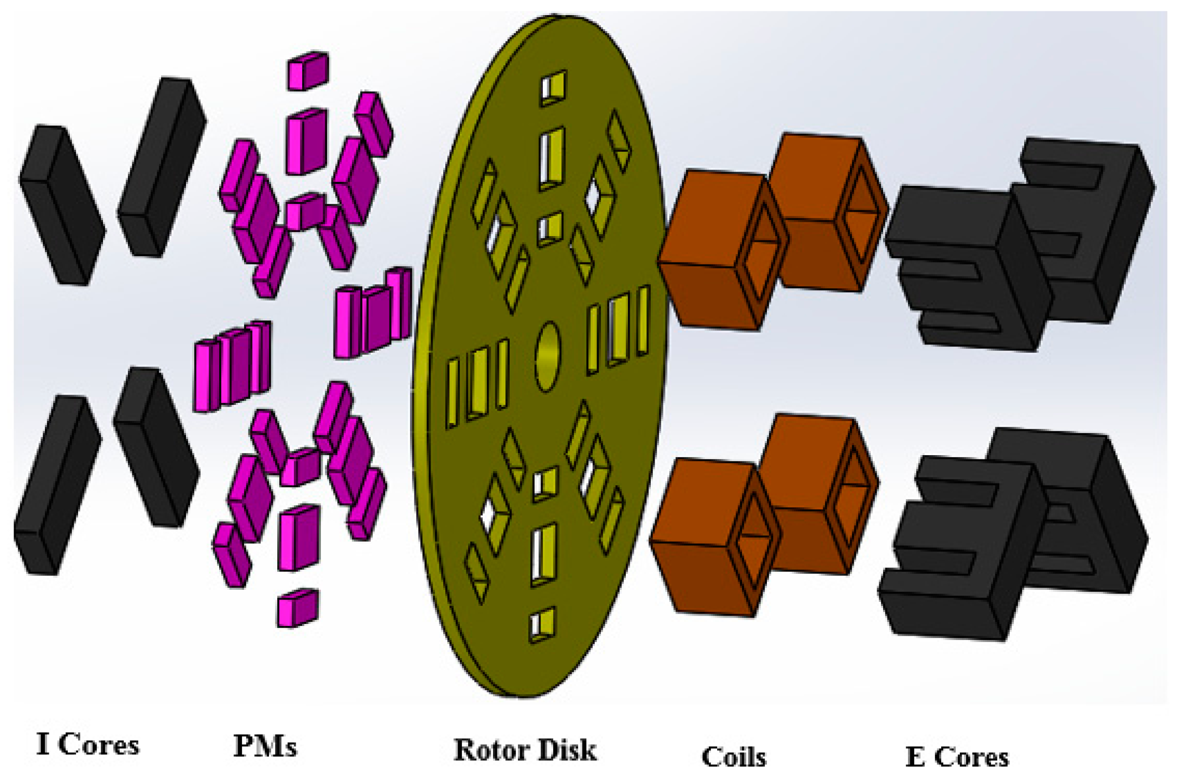
The general design of a single phase of this machine, as well as the introduction of different parts, is presented in Figure 1. In order to obtain a three-phase generator, three similar single phase modules (Figure 1), shifted in space by 120 electrical degrees, must be used [27].

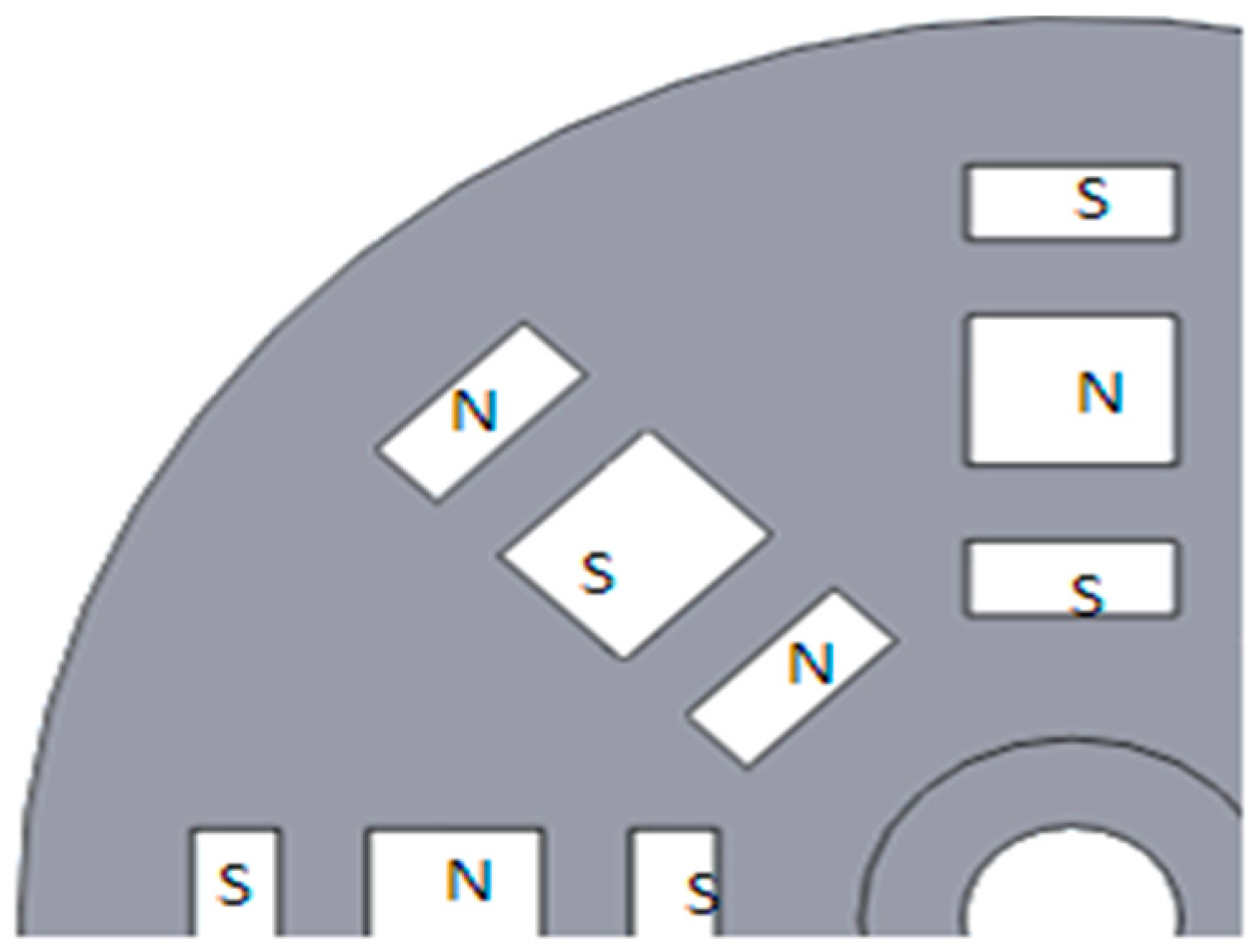
In this design, there are as many E and I-shaped cores as machine’s pole pairs. The winding of the machine is a simple coil, wrapped around the middle arm of the E-shaped core. These windings become parallel. As it has already been mentioned, having the same number of windings, pole pairs, and E & I-shaped cores, is one of the distinctive features that distinguish it from other structures of transverse flux machines. With this different structure, not only does getting higher output power become possible, but also, in case a winding gets in trouble, the generator can continue to operate with less power by removing that winding from the output circuit. On the other hand, having three rows of magnets, along with disk radius of the rotor, brings more equilibrium and balance for the rotor in the air gap length. The disk rotor of this machine is the place for permanent magnets. The disk of the rotor must be made of magnetic insulators in order to have a very little flux leakage between magnets over the disk, so that the flux easily enters into the air gap length. The placement of permanent magnets on the disk of rotor is depicted in Figure 2.

The stator body has the role of keeping the E and I-shaped cores fixed. The stator body material must be of magnetic insulators, to minimize the flux leakage between adjacent poles. All the dimensional parameters of this machine can be introduced in the following parts of the machine:

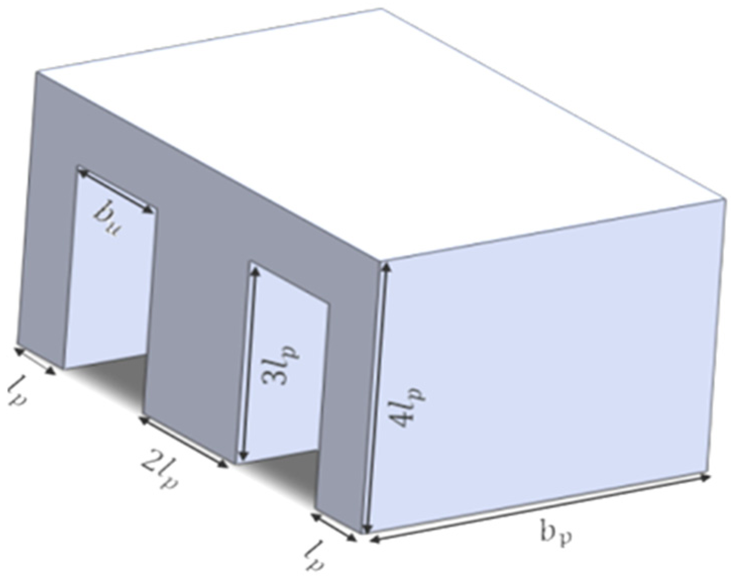
2.1. E-Shaped Core

The cross-sectional view of the E-shaped core is shown in Figure 3, with its dimensional parameters.

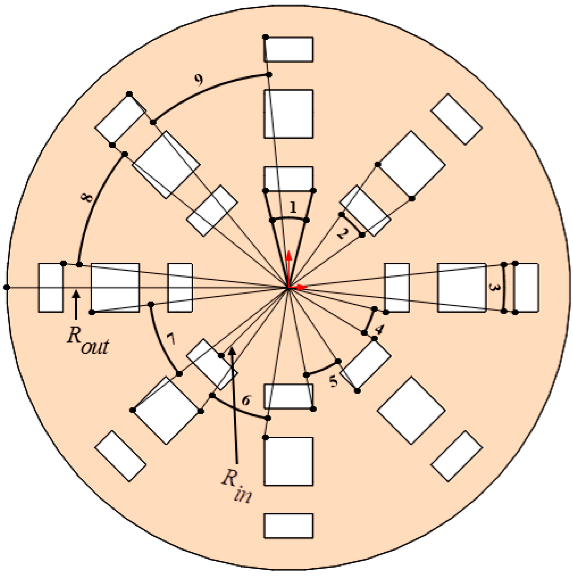
2.2. Rotor Disk Cross-Sectional View

The cross-sectional view of the rotor disk, along with its dimensional parameters, are shown in Figure 4.

Numerical parameters of Figure 4 are presented in

Table 1. Introducing determined dimensions in Figure 4.

Number	1	2	3	4	5	6	7	8	9
sign	$\alpha$	$\beta$	$\xi$	${\theta }_{g_1}$	${\theta }_{g_2}$	${\theta }_{g_3}$	${\theta }_{g_4}$	${\theta }_{g_5}$	${\theta }_{g_6}$

. It is noteworthy that the diameter of the rotor disk, which is similar to permanent magnet, is represented by the parameter $l_{pm}$.

3. The Algorithm of the Initial Design

In this section, the design process and basic dimensions of transverse flux permanent magnet machine are presented in detail. The mathematic equations used in the design are also proved or explained. The process of calculating dimensional parameters of the proposed machine, including obtaining nominal values and the main limitations, is as follows:

3.1. Main Design Parameters

The main design parameters are presented in

Table 2. The main design parameters.

Definition	Parameter	Value
Rated speed	$N_s[\mathrm{rpm}]$	750
Rated Power	$P_{out}[\mathrm{w}]$	200
Number of Phases	$m$	1
Frequency	$f[\mathrm{HZ}]$	50
Load Power Factor	$\cos \phi$	1
Rated Voltage (RMS (Root Mean Square))	$V_{out}[\mathrm{v}]$	70
Number of Poles	$p$	8

.

3.2. Adoptive Parameters

In a design problem, there might be cases in which some parameters must be selected as adoptive and independent ones. The values for these parameters must be selected considering items obtained by experience. In designing the machine, as unknown variables are more than equations, some design parameters are chosen as adoptive parameters, considering the definition of the problem and design limitations.

Adoptive parameters in the design of the proposed machine are presented in

Table 3. Adoptive parameters in designing the proposed machine.

Row	Definition	Parameter	Value
1	Coefficient current waveform	$k_i$	1.414
2	Coefficient power waveform	$k_p$	$0.5\cos \phi$
3	Magnetic relative permeability of vacuum	${\mu }_0$	$4\pi \times {10}^{-7}$
4	Magnetic relative permeability of E and I cores	${\mu }_r$	300
5	Magnetic relative permeability of permanent magnet	${\mu }_{rpm}$	1.0517
6	Ratio of $b_p$ to $l_p$	$k_l$	2.2727
7	Flux leakage coefficient in the air gap length	$k_{le}$	1.15
8	Ratio of distance between the center and side arm core of E-shaped ($b_u$) and the total length of the air gap lengths and the thickness of the permanent magnet ($l_{pm}+2g$)	$k_u$	1
9	The average of flux density in air gap length	$B_g\left[\mathrm{T}\right]$	0.8
10	Air gap length	$g\left[\mathrm{mm}\right]$	2
11	Residual flux density of the permanent magnet	$B_r\left[\mathrm{T}\right]$	1.32
12	Coercive force	$H_c\left[\frac{\mathrm{A}}{\mathrm{m}}\right]$	923000
13	Copper resistivity	${\mathsf{\rho }}_{cu}\left[\mathsf{\Omega }\cdot \mathrm{m}\right]$	$2.0052\times {10}^{-8}$
14	Current density	$J\left[\frac{\mathrm{A}}{{\mathrm{mm}}^2}\right]$	9

.

3.3. Computational Parameters

In this section, the machine’s dimensions are designed using the presented equations in each section.

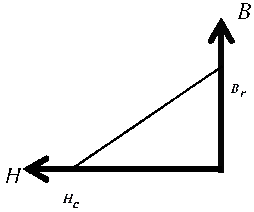
3.3.1. Computing the Thickness of the Permanent Magnet

To calculate the thickness of the permanent magnet, an equivalent magnetic circuit is used at the instance when the permanent magnets are placed exactly across the E-shaped core. The curve for changes of flux density over magnet according to the intensity of the permanent magnet field is shown in Figure 5.

Magnetic permeability coefficient of the permanent magnet (µ_pm) can be calculated from Figure 5. In fact, it can be said that µ_pm is the line slope of Figure 5. Accordingly, magnetic permeability coefficient of the permanent magnet (µ_pm) and its relative magnetic permeability coefficient (µ_rpm) are defined as Equations (1) and (2), respectively.

$${\mu }_{pm}=\frac{B_r}{H_c}={\mu }_{rpm}{\mu }_0$$

(1)

$${\mu }_{rpm}=\frac{{\mu }_{pm}}{{\mu }_0}=\frac{B_r}{{\mu }_0{H}_c}$$

(2)

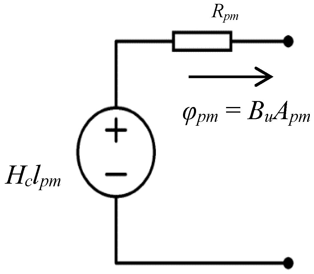
According to the above equations, the permanent magnet can be modeled as the magnetic Thévenin equivalent circuit shown in Figure 6.

In Figure 6, R_pm parameter represents interior reluctance of permanent magnet, and its value is calculated by Equation (3).

$$R_{pm}=\frac{H_c{l}_{pm}}{B_r{A}_{pm}}=\frac{l_{pm}}{{\mu }_{pm}{A}_{pm}}=\frac{l_{pm}}{{\mu }_0{\mu }_{rpm}{A}_{pm}}$$

(3)

According to the equivalent permanent magnet circuit and equivalent magnetic circuit of the machine, Equation (4) can be extracted for computation of permanent magnet thickness:

$$l_{pm}=\frac{2\times B_g\times B_r\times g}{H_c\times \left(B_r-B_g\right)\times {\mu }_0}$$

(4)

3.3.2. Computation of RMS (Root Mean Square) Current of Each Pole of the Machine

The RMS of current for each pole can be calculated through Equation (5):

$$I_{rmsp}=\frac{P_{out}}{(p/2)V_{out}cos\phi }$$

(5)

3.3.3. Computation of Fundamental Component Amplitude of the Induced Voltage in Each Winding Turn for the Proposed Design

According to changes of $k_l$ and $K_u$ coefficients, the following modes can be considered for presented angles in Figure 4:

$$\beta \ge ({\theta }_{g5}+\xi )/2\to \left\{\begin{array}{c}\xi \ge {\theta }_{g5}>{\theta }_{g3}>{\theta }_{g1}\\ {\theta }_{g5}>\xi \ge {\theta }_{g3}>{\theta }_{g1}\\ {\theta }_{g5}>{\theta }_{g3}>\xi \ge {\theta }_{g1}\\ {\theta }_{g5}>{\theta }_{g3}>{\theta }_{g1}>\xi \end{array}\right\}$$

$$\beta <({\theta }_{g5}+\xi )/2\to \left\{\begin{array}{c}\xi \ge {\theta }_{g1}\\ {\theta }_{g1}>\xi \end{array}\right\}$$

The steps in obtaining fundamental component amplitude of voltage for the first mode are explained here as an example:

Step one: in this step, the flux linking all winding turns of each pole, which is generated by the permanent magnet, is calculated at different rotor positions (the following positions):

(A).

The first position: the entire surface of the magnet across the E-shaped core (${\phi }_1$ flux)

(B).

The second position: a rotor displacement of ${\theta }_{g1}$ compared to the first position (${\phi }_2$ flux)

(C).

The third position: a rotor displacement of ${\theta }_{g3}$ compared to the first position (${\phi }_3$ flux)

(D).

The fourth position: a rotor displacement of ${\theta }_{g5}$ compared to the first position (${\phi }_4$ flux).

(E).

The fifth position: a rotor displacement of $({\theta }_{g5}+\xi )/2$ compared to the first position (${\phi }_5$ flux)

Step two: in this step, the voltages induced in each winding turn are calculated by derivation from flux diagram, considering rotor position (Equations (6)–(9)):

$$e_1=\frac{4\pi f\times \left({\phi }_1-{\phi }_2\right)}{p\times {\theta }_{g1}}$$

(6)

$$e_2=\frac{4\pi f\times \left({\phi }_2-{\phi }_3\right)}{p\times \left({\theta }_{g3}-{\theta }_{g1}\right)}$$

(7)

$$e_3=\frac{4\pi f\times \left({\phi }_3-{\phi }_4\right)}{p\times \left({\theta }_{g5}-{\theta }_{g3}\right)}$$

(8)

$$e_4=\frac{4\pi f\times \left({\phi }_4-{\phi }_5\right)}{p\times \left(\xi -{\theta }_{g5}\right)}$$

(9)

Step three: in this step, the fundamental component amplitude of the voltage induced in each winding turn for the proposed design is calculated using Fourier series (Equation (10)):

$$E_{11maxp}=\left(\frac{4}{\pi }\right)\times \left(\begin{array}{c}{e}_1\times \left(1-\cos ((p\times {\theta }_{g1})/2))\right)+\\ \begin{array}{c}{e}_2\times \left(\cos ((p\times {\theta }_{g1})/2))-\cos ((p\times {\theta }_{g3})/2))\right)+\\ \begin{array}{c}{e}_3\times \left(\cos ((p\times {\theta }_{g3})/2))-\cos ((p\times {\theta }_{g5})/2))\right)+\\ e_4\times \left(\cos ((p\times {\theta }_{g5})/2))\right)\end{array}\end{array}\end{array}\right)$$

(10)

3.3.4. Presenting the Output Equation for the Proposed Design

The output power of any electric machine can be computed by using Equation (11), ignoring the synchronous reactance and winding resistance [29]:

$$P_{out}=m(\frac{p}{2})k_i{k}_p{N}_p{E}_{11maxp}{I}_{rmsp}$$

(11)

The presence of $(\frac{p}{2})$ in Equation (11) is because of the fact that the number of paired poles and windings in this machine are the same.

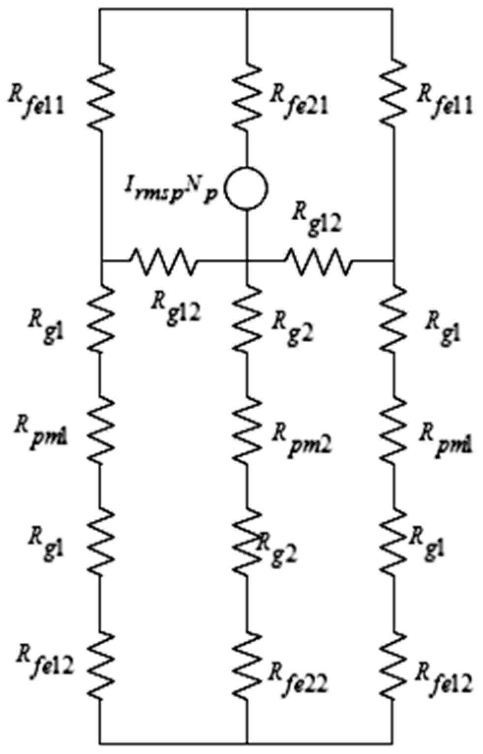
3.3.5. Computation of Synchronous Reluctance in Each Winding Turn (Initial Synchronous Reluctance)

To calculate initial synchronous reluctance, the following steps must be taken:

Step one: in this step, the reluctance observed across the winding must be obtained. For this purpose, the magnetic equivalent circuit given in Figure 7 must be used. The reluctance observed across the winding is represented by $R_t$.

The value for each definite reluctance of Figure 7 is computable using Equations (12)–(20):

$$R_{fe11}=\frac{b_u+5l_p}{{\mu }_0{\mu }_{rfe}{l}_p{b}_p}$$

(12)

$$R_{fe12}=\frac{b_u+2.5l_p}{{\mu }_0{\mu }_{rfe}{l}_p{b}_p}$$

(13)

$$R_{fe21}=\frac{3.5l_p}{2{\mu }_0{\mu }_{rfe}{l}_p{b}_p}$$

(14)

$$R_{fe22}=\frac{0.5l_p}{2{\mu }_0{\mu }_{rfe}{l}_p{b}_p}$$

(15)

$$R_{g1}=\frac{g}{k_{le}{\mu }_0{l}_p{b}_p}$$

(16)

$$R_{g2}=\frac{g}{2k_{le}{\mu }_0{l}_p{b}_p}$$

(17)

$$R_{g12}=\frac{b_u}{k_{le}{\mu }_0(2g+lpm)b_p}$$

(18)

$$R_{pm1}=\frac{l_{pm}}{{\mu }_{rpm}{\mu }_0{l}_p{b}_p}$$

(19)

$$R_{pm2}=\frac{l_{pm}}{2{\mu }_{rpm}{\mu }_0{l}_p{b}_p}$$

(20)

Step two: in this step, the initial inductance of the winding, and the initial synchronous reactance, can be calculated using the obtained reluctance in the previous step, through Equations (21) and (22):

$$L_{t1}=\frac{1}{R_t}$$

(21)

$$X_{s1}=2\pi f{L}_{t1}$$

(22)

3.3.6. Computing Wire Diameter and the Resistance in Each Winding Turn (the Initial Resistance) of the Winding $R_{a1}$

Firstly, considering the current density of the copper conductor, the cross-sectional area of the wire is computed by Equation (23), in order to determine the wire diameter:

$$A_{cuw}=\frac{I_{rmsp}}{J}$$

(23)

Now, if the conductor cross-section is considered to be circular, wire diameter will be calculated according to Equation (24):

$$D_w=2\sqrt{\frac{A_{cuw}}{\pi }}$$

(24)

To calculate the winding initial resistance, the resistivity of copper is used (Equation (25)):

$$R_{a1}=\frac{1.65{\rho }_{cu}\left(2l_p+2b_p\right)}{A_{cuw}}$$

(25)

3.3.7. Computing Final No Load Voltage of the Generator

The fundamental harmonic of final no load voltage, $E_f$(RMS), will be calculated according to Equation (26):

$$N_p=\frac{E_f}{V_{out}}$$

(26)

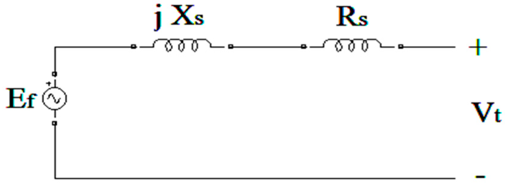
The number of winding ($N_p$) can be calculated using the synchronous machine equivalent circuit presented in Figure 8, and the nonlinear Equation (27):

$$N_p{V}_{out}-\left|\left(N_p{R}_{a1}+j{N}_p^2{X}_{s1}\right)I_{rmsp}{e}^{-j\phi }+V_{out}\right|=0$$

(27)

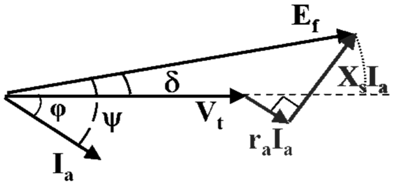
3.3.8. Computation of Machine’s Power Angle ($\delta$) in Full Load Mode

Figure 9 shows a vector diagram of the generator’s voltage in leading mode.

The machine’s power angle can be calculated using the voltage vector diagram of the machine and Equation (28).

$$\delta =ta{n}^{-1}\left(\frac{X_s{I}_{rmsp}cos\phi -R_a{I}_{rmsp}sin\phi }{V_{out}+X_s{I}_{rmsp}sin\phi +R_a{I}_{rmsp}cos\phi }\right)$$

(28)

The flowchart of the proposed TFPMDEIG for the initial design is shown in Figure 10.

Using all the design equations presented above, all dimensions and parameters of the machine are calculated. These dimensions are shown in

Table 4. Machine’s dimensions and computational parameters.

Row	Definition	Parameter	Value
1	Inner radius of the rotor disk	$R_{in}\left[\mathrm{mm}\right]$	40.1
2	Outer radius of the rotor disk	$R_{out}\left[\mathrm{mm}\right]$	120
3	Thickness of permanent magnet	$l_{pm}\left[\mathrm{mm}\right]$	7
4	Size of the core of E-shaped side arm	$l_p\left[\mathrm{mm}\right]$	11
5	Thickness of E-shaped core	$b_p\left[\mathrm{mm}\right]$	25
6	The length between the middle and the side arm of E-shaped core	$b_u\left[\mathrm{mm}\right]$	11
7	Turns of winding	$N_p$	1450
8	Main harmonic of induced voltage	$E_f\left[\mathrm{V}\right]$	115.28
9	Resistance	$R_a[\mathsf{\Omega }]$	46.54
10	Synchronous Reactance	$X_s[\mathsf{\Omega }]$	50.03
11	Power angle	$\delta °$	19.84

.

4. Finite-Element Analysis (FEA)

3-D FEM is employed to analyze the magnetic circuit. The investigation provides an overall depiction of the different parts of the suggested generator saturation levels, and excerpts their characteristics. The fundamental FEA equations are presented as Equation (29)–(31) [30].

$$\nabla \times \overrightarrow{B}=\mu \overrightarrow{J_s}$$

(29)

$$\nabla \times \overrightarrow{J_s}=-\sigma \frac{d\overrightarrow{B}}{dt}$$

(30)

$$\overrightarrow{B}=\nabla \times \overrightarrow{\mathsf{\Psi }}$$

(31)

where $\overrightarrow{B}$, $\overrightarrow{J_s}$, $\overrightarrow{\mathsf{\Psi }}$, $\sigma$, and $\mu$, are the magnetic flux density, current density, magnetic vector potential electrical conductivity, and magnetic permeability, respectively. If $\overrightarrow{H}$ is taken as the magnetic field intensity, previous equations result in Equation (32):

$$\nabla \times \left(\frac{1}{\sigma }\nabla \times \overrightarrow{H}\right)+\frac{\partial \overrightarrow{B}}{\partial t}=0$$

(32)

where the vector fields are represented by first-order edge elements, and the scalar fields by second-order nodal unknowns. Field equations are combined with circuit equations for conductors. The numerical solutions of Equations (29)–(31) involve a finite element discretization methodology. Due to the complexity of magnetic field distribution in the axial and radial spaces of TFPMDEIG, the 3-D FEM is employed to analyze its electromagnetic characteristics. Three-dimensional FEM perfectly calculates the different components of the flux density. The design was simulated using the JMAG Designer 10.5 software package (JSOL Corporation, Tokyo, Japan).

The first step in modeling by means of 3-D FEM is to draw the geometry of the problem. This can be done by tools in the software, or by a drawing technical software, such as Solid Works. Figure 11 shows the drawn geometry of a pair of poles in this generator.

The proposed generator in this paper has 8 poles, and the magnetic and geometric pattern of a pair of poles is repeated according to the number of paired poles. Therefore, modeling only a pair of poles is enough for balanced performance analysis and achieving the desired goals. After geometric drawing, the material for each section must be determined. This is done considering

Table 5. Properties for material of the TFPMDEIG.

Generator Parts	Material
E and I cores	Laminated steel with permeability coefficient 300
Rotor Core	Paper sheet with phenolic resin
Permanent Magnet	NeFeBr 45
Winding	Copper

.

It must be noted that it is possible to use SMC, instead of laminated steel, for construction of the E and I cores. In this research, however, SMC was not used for the following reasons:

(1)

The low frequency and the rotor’s low rotation speed,

(2)

The severe difficulties with acquiring SMC cores in a small quantity.

5. Simulation Results

After finishing the processing stage, the step for extracting the results, known as post-processing, starts.

Simulation results are presented in two steps, i.e., static and dynamic analyses.

5.1. Static Analysis

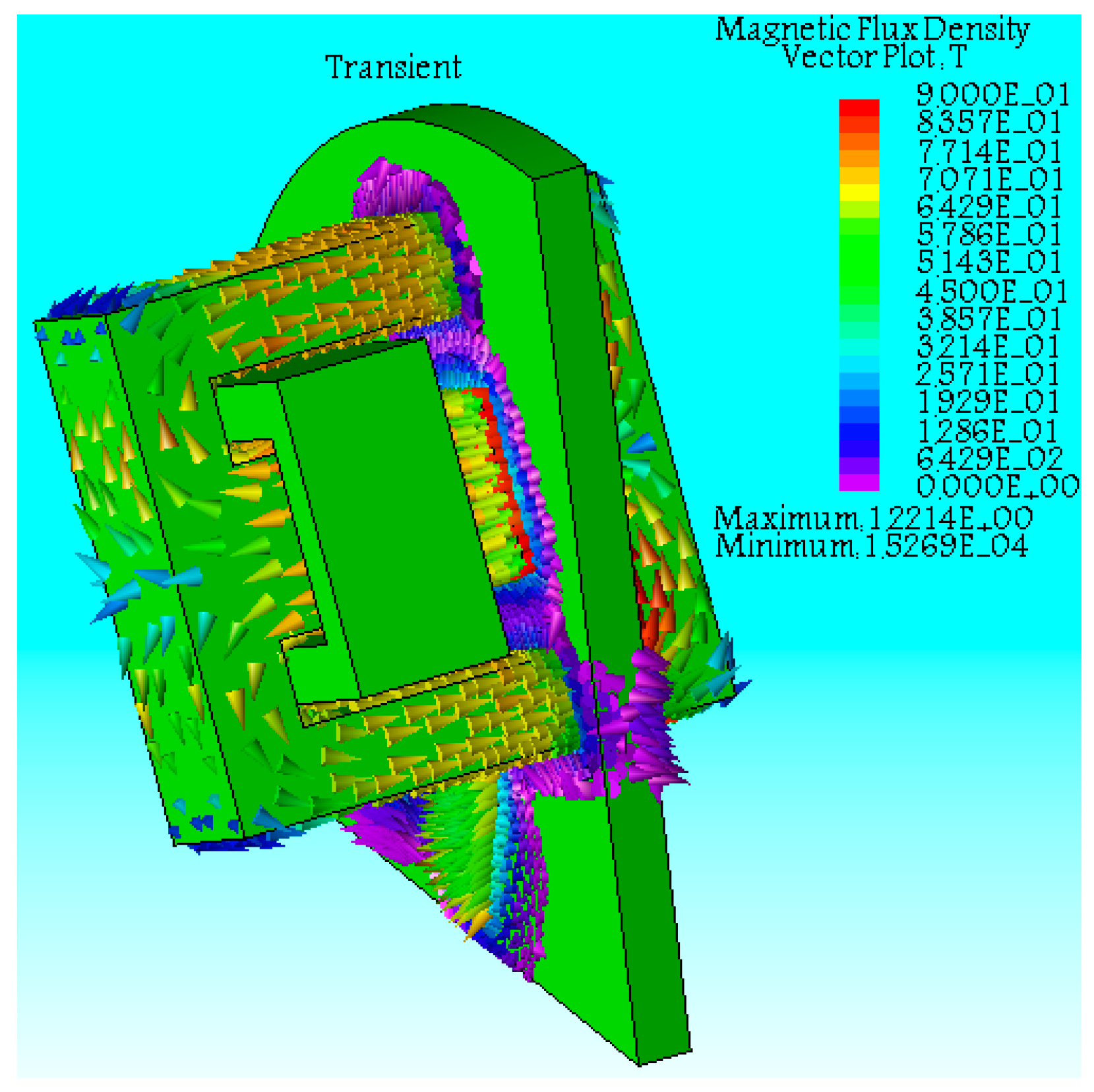
Currents in windings are considered to be zero, and magnets are exactly opposite the E-shaped cores. In this mode, an operating point with average flux density of 0.800123 Tesla is obtained. On the other hand, by changing the winding current from minimum to maximum, the operating point changes from 0.6563 to 0.9437 Tesla.

In open circuit mode, the distribution of flux density is only because of magnets. Figure 12, as a contour plot, shows the distribution of flux density of magnetic field in initial rotor position.

Also, in this mode, the lines of magnetic flux density in a pair of pole of the machine are shown in Figure 13.

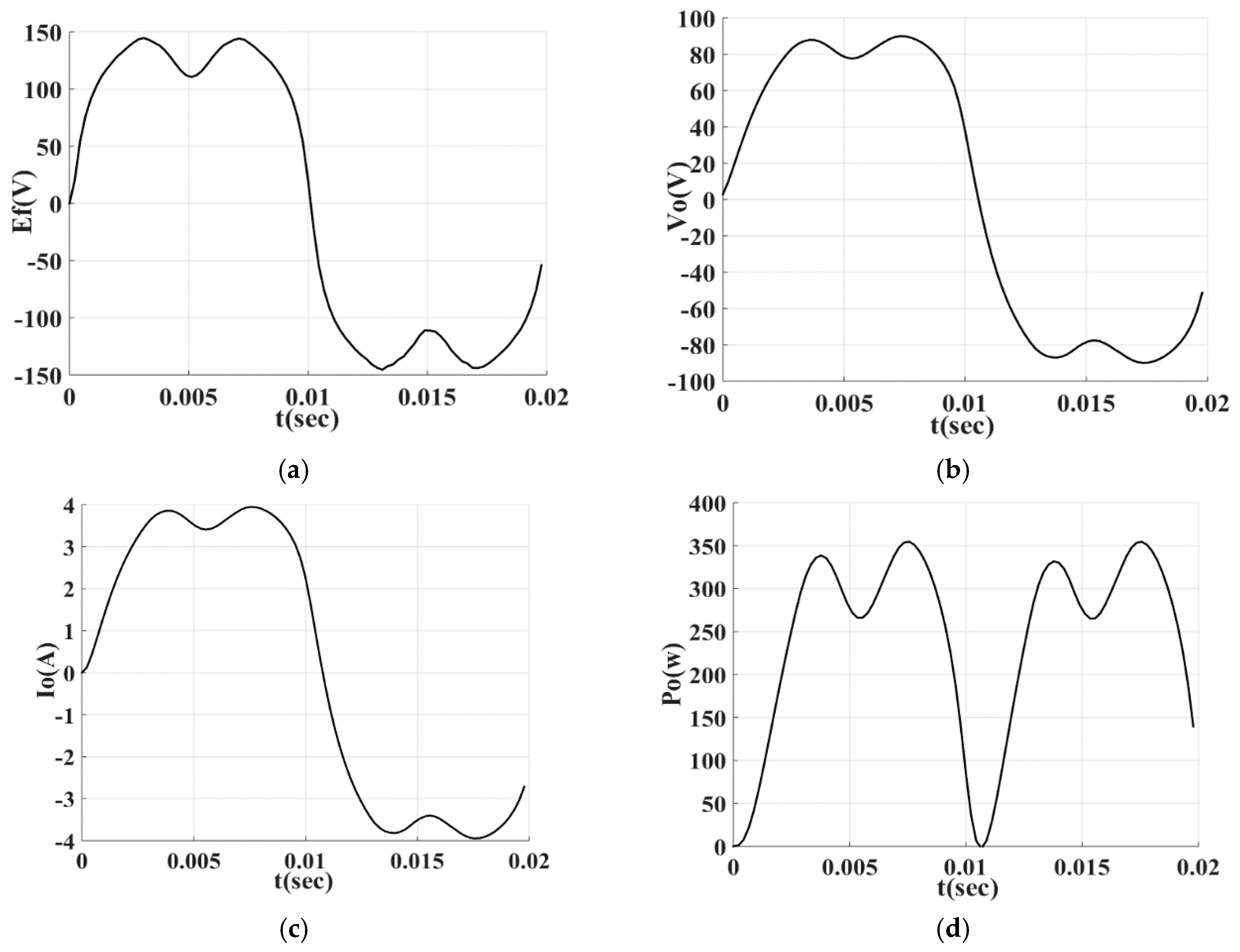
5.2. Dynamic Analysis

The no-load voltage curve, the output voltage curve, output current curve, and output power curves at full load are plotted in Figure 14.

More analysis on results from 3-D FEM is discussed in Section 7.

6. Prototyping and Testing of the Designed TFPMDEIG

A prototype is fabricated to assess the validity of the proposed TFPMDEIG. The experimental results are in good agreement with the 3-D FEM analyses. The fabricated TFPMDEIG is shown in Figure 15a. The manufacture of the proposed generator can be described in the following three steps:

1-

Rotor disk: The rotor disk is made of paper sheet with phenolic resin (Figure 15b). Permanent magnets have been fixed by glue on it.

2-

The stator body: the stator body is made of compact plastic with a thickness of 25 mm. The stator body holds the stator cores (E and I core) (Figure 15c,d). The location of the stator core is carved by CNC (computer numerical control) milling machine.

3-

E and I-shaped cores: E and I-shaped cores are made of silicon steel. In order to reduce core losses, E and I-shaped cores are laminated.

Figure 16 shows the experimental platform of the TFPMDEIG, consisting of an inverter drive (VFD (variable-frequency drive)), an asynchronous motor, the TFPMDEIG, a resistive load and an oscilloscope. The prototype is driven by the asynchronous motor, which is fed by the frequency converter. Experiments on the TFPMDEIG are of two types; no load, and load tests. In the latter case, a resistive load is used.

The no-load voltage curve, output voltage curve, output current curve, and output power curves at full load, are plotted in Figure 17.

7. More Results and Discussion

Table 6. Key motor parameters.

Definition	Parameter	Initial Algorithm Results	3D-FEA Results	Experimental Results
No load voltage (Amplitude)	$E_f^{\max }[\mathrm{V}]$	171.35	169.36	164.78
Main harmonic no load voltage (Amplitude)	$E_{f1}^{\max }[\mathrm{V}]$	163.03	161.77	158.42
Output voltage (Amplitude) for full load	$V_{ofl}^{\max }[\mathrm{V}]$	101.23	105.32	98.30
Main harmonic full load voltage (Amplitude)	$V_{o1fl}^{\max }[\mathrm{V}]$	98.99	102.05	96.19
Full load current (Amplitude)	$I_{ofl}^{\max }[\mathrm{V}]$	4.49	4.46	4.26
Main harmonic full load current (Amplitude)	$I_{o1fl}^{\max }[\mathrm{V}]$	4.68	4.60	4.31
THD * of no load voltage	THD	28.12%	30.99%	29.06%
THD output voltage in full load condition	THD	24.52%	25.54%	15.49%
THD output current in full load condition	THD	24.52%	25.42%	15.19%
Armature Resistance	$R_a[\mathsf{\Omega }]$	11.63	-	11.8
Synchronous Reactance	$X_s[\mathsf{\Omega }]$	12.51	13.63	14.11
No load voltage (Effective value)	$E_f[\mathrm{V}]$	115.28	114.02	112.01
Output voltage (Effective value) for full load	$V_{ofl}[\mathrm{V}]$	70	72.12	68.02

* Total Harmonic Distortion.

summaries the key parameter comparison between the initial algorithm, 3D-FEM, and experiment results. It can be seen that the analysis results of the TFPMDEIG match well with the experiment ones.

It can be seen that voltage THD or current THD is high. This phenomenon in the proposed generator looks normal, because the air gap length is high. To decrease THD, the generator must be made with a high number of poles.

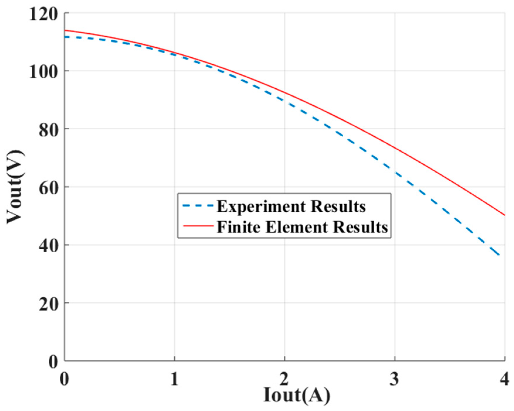
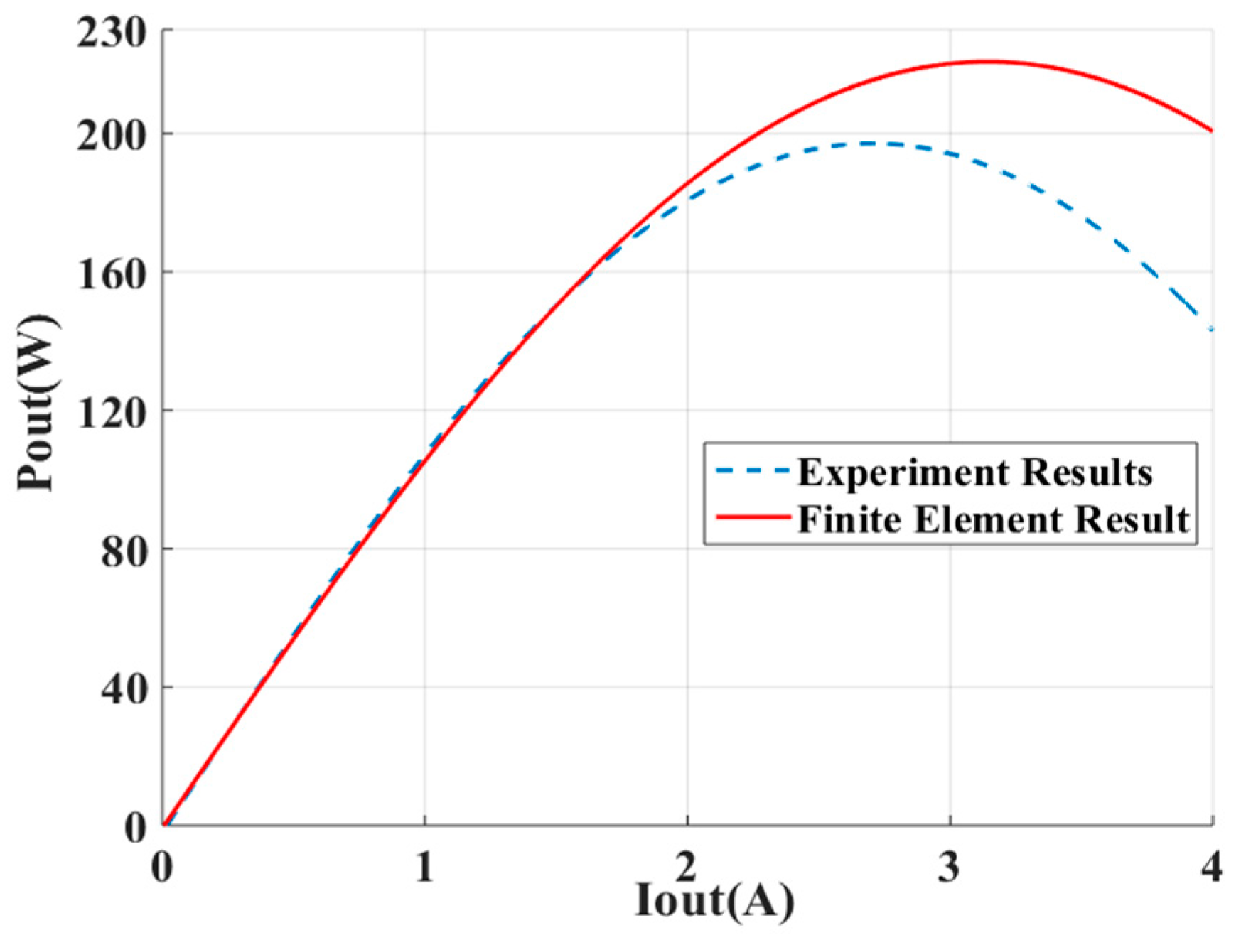
Figure 18 shows the variation of the output voltage versus load current. Figure 19 shows the output power versus the load current. With increasing load current, and approaching the rated current, the difference between the FEA results and the experimental results becomes larger. The 3-D FEM results and the experimental results are thus in good agreement, up to the nominal current. If the current is increased further than this value, then the errors become more substantial. The main contributors to the discrepancies between the FEA results and the experimental results are as follows: (a) weakening of the PMs; difference between the no-load voltages obtained from the 3D-FEA and the experimentally measured no-load voltage (Figure 19 for $I_{out}=0$) settles the weakening of the PMs; (b) armature resistance increases with the heat produced by passing current through the winding; (c) three dimensional leakage flux pathways. These pathways affect the synchronous reactance.

8. Conclusions

A new structure for a transverse flux permanent magnet generator has been presented. This generator, in addition to the advantages of transverse flux machines, has the benefits of a disk machine. In general, the disk structure has the following advantages: (1) allows for high rotational speeds; (2) makes the manufacture simpler, by using laminated steel sheets. The generator design was initially done by theoretical analysis, based on the initial algorithm. A typical low power TFPMDEIG was designed. The obtained parameters for the TFPMDEIG were verified by the model analysis via 3D-FEM. The 3D-FEM modified and moderated the design parameters based on electromagnetic field analysis. The flux density agreed well in air gap length of the proposed generator, which was compared between 3-D FEM and initial algorithm results at no-load condition. The dynamic electromagnetic analysis of the TFPMDEIG was performed in different loads, and the variation of output power and output voltage versus current was obtained. The generator was fabricated, and the resulting prototype TFPMDEIG was subjected into the experimental test. For nominal condition, there is a good agreement between the simulations and the experimental results. As the load current increases beyond the nominal value, the discrepancies between the simulations and the experimental results become greater. One of the major reasons for these discrepancies is that the PMs used in the experimental setup were weaker than those used in the simulations. Additionally, as the load current increases, the temperature of the armature windings increases, causing the armature resistance to rise. This was not accounted for during the simulations.