Energy Prediction of Access Points in Wi-Fi Networks According to Users’ Behaviour

Abstract

Some maintenance tasks in Wi-Fi networks may involve removing an access point due to several reasons. As a result, the new infrastructure registers a different number of roamings in the access points according to the users’ behaviour, with a certain energy impact added to the consumption caused by the own operations of the devices. This energy effect should be understood in order to tackle the measures aimed at planning the infrastructure deployment. In this work, we propose a methodology to predict the energy consumption in the access points of a Wi-Fi network when we remove a particular device, based on a twofold support. We predict the number of roamings following a method previously validated; on the other hand, we assess the relationship between roamings and energy in the full infrastructure, using the data collected from a high number of network users during a given time in order to reflect the users’ behaviour with the maximum accuracy. From this knowledge, we can infer the energy prediction for a different environment where the roamings are predicted using techniques based on recommender systems and machine learning.

1. Introduction

The Access Point (AP) is one of the most important communication devices present in Wi-Fi networks. In any wireless network deployment, maintenance or enhance task, it is desirable to preserve a good balance between economic cost and performance, especially when we deal with environments subjected to a high number of users, such as a university campus, where students, professors and employees demand a lot of network resources. The economic cost comes from not only the number of devices and their unitary cost, but also the workload due to the users demanding network access through APs.

The usual operations of the APs involve certain energy levels, different for each device according to its location and physical characteristics. Usually, current APs are powered by Power Over Ethernet (PoE) systems, which transmit data and electric power together using Ethernet cables. This technology speeds up the network deployment, with the corresponding cost savings due to the reduction of the materials needed. The possibility to use the popular RJ-45 Ethernet connector for this purpose [1] simplifies the maintenance works of the infrastructure and allows the control and measurement of both data and energy in the AP by means of a specialised software. Thus, software tools can assign the power in the APs analysing the frequency spectrum in order to select the optimal power and channel, according to the interferences and regional rules. Nevertheless, once this power basis is selected, the main source of variability in the energy levels come from the operations oriented to satisfy the demand of network access by the users. In this work, we focus our research interest in this second energy component, where the energy is strongly related with the users’ activity.

The users’ activity can be registered using software tools that monitor modern wireless networks. These tools identify the interaction between users and APs, as well as the energy levels in the devices. The longer we monitor the network, the more data we obtain. A careful study of this data can give us valuable information about the users’ behavior and its effect on the energy levels in the APs. This information is useful for planning the network deployment or enhancing it through maintenance tasks related with the APs, whose energy impact should be previously evaluated.

Particularly, in this work we focus our attention on general maintenance, consisting of removing a determined AP due to changes in the organisation of spaces, rooms and buildings (which is very usual in academic environments). This removal produces a certain energy impact on the remaining APs in the network, coming from the users’ behavior when they request network access, resulting in a different infrastructure. In this situation, if we knew how the energy pattern of the network would be after removing a determined AP, we could study which of the remaining APs should be reinforced if the energy consumption increases too much. This reinforcement can be either adding another device to the proximity of the punished AP, or replacing it with another device with higher performance. Both possibilities imply a new expense. Therefore, predicting the energy consumption is very useful for us in order to analyse determined situations with the purpose of reducing economic costs and guaranteeing the quality of service.

What is the energy impact in the APs after removing one of them? This question can be answered by predicting the number of roamings for the new infrastructure and establishing a relationship between the number of roamings and the energy levels in the access points. For this purpose, it is necessary to collect data of the network usage by a high number of network users during enough time in order to reflect the users’ behavior with the maximum accuracy. From this knowledge, we can infer the energy prediction for a different environment where the roamings are predicted using techniques based on machine learning and big data analysis. In this sense, the relevance of our proposal lies in predicting the energy in the APs through a novel method that connects this energy with the predicted roamings after removing an AP, considering a relationship based on point coefficients.

Within the wide range of prediction techniques in the machine learning field, Recommender Systems (RS) [2] are good choice upon which to base the roamings’ prediction and, from it, the energy prediction of the APs. Recommender Systems represent a well-proven prediction technique because they analyse in depth the relationship between users and tasks, evaluated by scores or performances. In our case, we consider the relationship between network users and access points, evaluated by the number of roamings that each user registers in each AP; therefore, the users’ habits are strongly considered in the prediction.

The remainder of this paper is structured as follows. After going over some related works in Section 2, Section 3 presents a novel methodology for predicting the energy impact on the APs after removing a particular device, based on the roamings prediction for the resulting infrastructure. In Section 4, we detail the experimental framework based on a real-world wireless environment where a great amount of data was collected, that is analysed in Section 5. Next, we present in Section 6 the results of the energy prediction according to the methodology described before. Section 7 presents an experimental validation of the proposed prediction method. Last, a discussion of the results is left for Section 8.

2. Related Works

Access Points play an important role in the planning, prediction or optimisation of wireless networks. Several of these aspects, such as optimal location and radio characteristics of the devices, have a certain effect on the energy levels of the APs and other communication elements. For example, there are methods for reducing power consumption in communication terminals by adjusting the radio transmission range [3] and for minimising the energy consumption in wireless networks [4]. Other aspects related with users’ behaviour have an energy impact too. Our work focuses on the connection between the number of roamings established by the users and the energy consumption in the APs. Like this focus, security levels and energy consumption are connected in a module for the Internet of Things (IoT) based on Wi-Fi protocol [5].

Many prediction tasks for the deployment or maintenance of Wi-Fi networks consider APs as a basic element to take into account. Thus, predicting the density of neighbouring APs and the corresponding data traffic of Wi-Fi networks [6] allows the sharing of cellular and Wi-Fi networks in the same spectrum [7], and the prediction of the data quota that user management facilitates to design network infrastructures where data pricing is significant [8].

The prediction efforts in wireless networks also focus on the users’ location and data traffic. Principally, a location prediction method based on nonlinear time series analysis of the arrival and residence times of users in relevant places is applied to predict their future movements [9]. Secondly, a method that considers terminal distribution to predict the throughput of an AP in a simulated network is proposed in [10]. In addition, although we could know the traffic demand (with the corresponding energy impact), it is difficult to predict it due to its highly dynamic nature, which should be considered when applying routing solutions. For example, tools for network routing under dynamic data demand are shown in [11], where the traffic is predicted by studying the traces collected at APs by means of time series analysis; and a network-based routing algorithm [12] and a meta-director framework [13] were developed to obtain optimal paths in cloud computing massive infrastructures in order to minimise the energy consumed by the users’ requests.

Mobility and services are also predicted in wireless networks. For example, mobility is described in [14] by the mobile node’s next AP using prediction agents related to an AP in Wi-Fi networks. Besides, there are networks where the demand of resources and services can be predicted for optimisation tasks. Thus, application workloads in enterprises are predicted in [15] considering performance modelling and capacity planning, according to demand patterns in order to design recommendation services.

Our prediction methodology finds common points with other works where, although they consider different aspects of the Wi-Fi networks, machine learning and big data analysis offer an interesting starting point to predicting tasks. For example, statistical [16] and learning methods [17] are considered for prediction purposes, like traffic patterns and database workloads.

The optimal placement of wireless devices, such as APs or routers, has been also widely studied in [18]. These studies are interesting for our purposes. The initial deployment of the APs can determine the probablity of a determined device to be removed facing certain maintenance works as space reorganisation. Thus, if we have different options to plan initial deployments, we should choose the solution that offers less probability of assigning APs in places with a high risk to be changed in the future (for example, proximity to divisible rooms). Many of these studies of initial optimal deployments consider different parameters as optimisation goals; for our interest, we should consider coverage [19], rather than lifetime, economic cost, failure risks, etc.

Lastly, we mention a previous work where we validated a methodology based on Recommender Systems (RS) for predicting the number of roamings in the APs [20] after removing one of them. As many wireless networks cannot collect energy data from the APs, we can take advantage of this previous work in order to initialise a new approach for predicting energy data, where we establish a quantified relationship between the number of roamings and the energy consumption.

3. An Energy Prediction Proposal

We propose a methodology for predicting the energy in the APs once one of them has been removed from the wireless network, considering the data (energy and roamings) collected previously during a large period. This methodology starts from the prediction of the number of roamings for the simulated infrastructure. Next, we study the relationship between this number and the energy used in the APs in order to propose a new approach to the energy prediction of the APs in such scenario.

Figure 1 shows the prediction proposal, which consists of three phases for the prediction works: Studying the current network status and the relationship between number of roamings and energy use in the APs (phase #1); predicting the number of roamings after removing an AP (phase #2); and predicting energy use of the APs in the new infrastructure (phase #3). The figure shows an additional work with regard to the experimental validation, which will be explained in a later section.

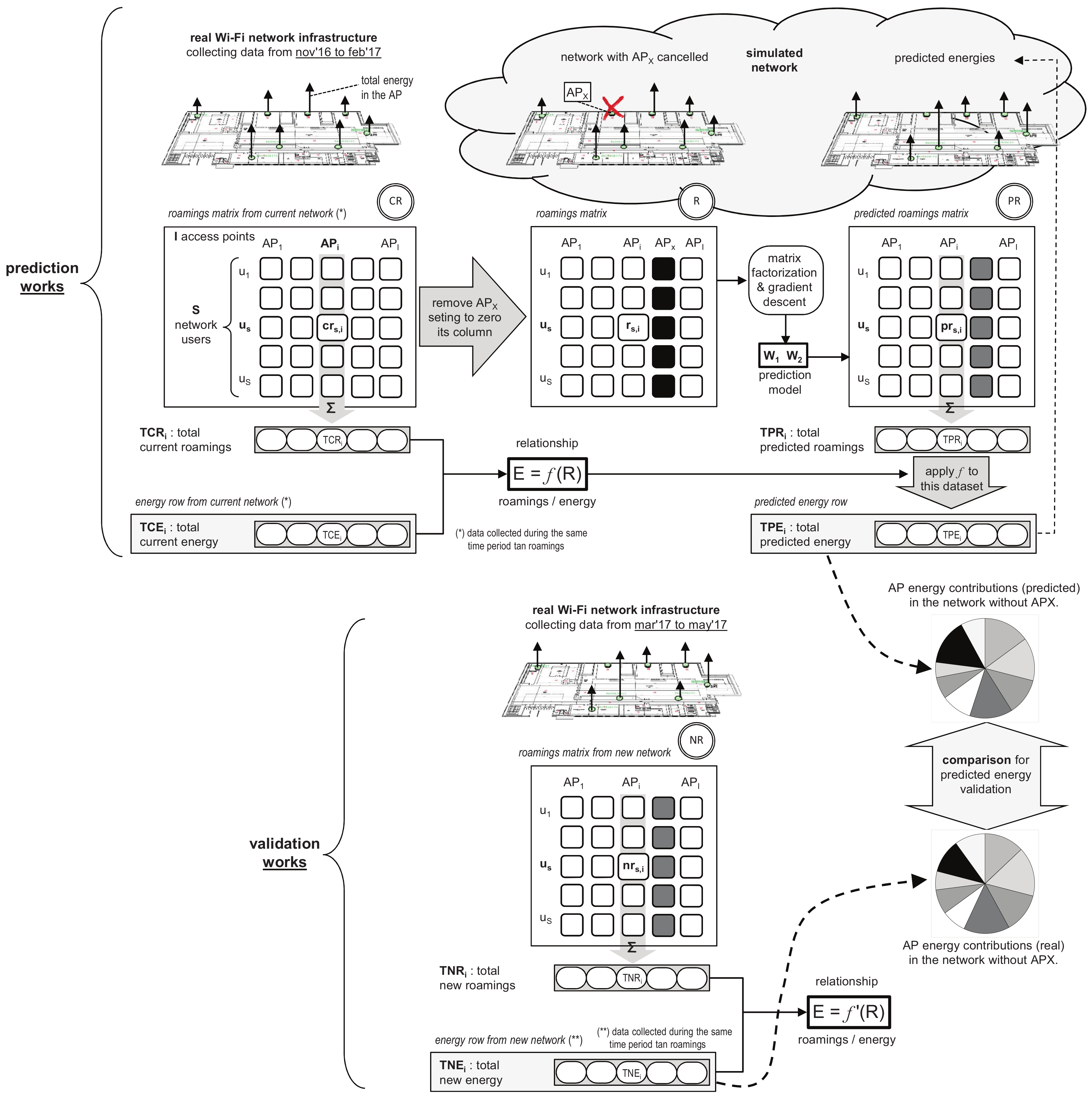
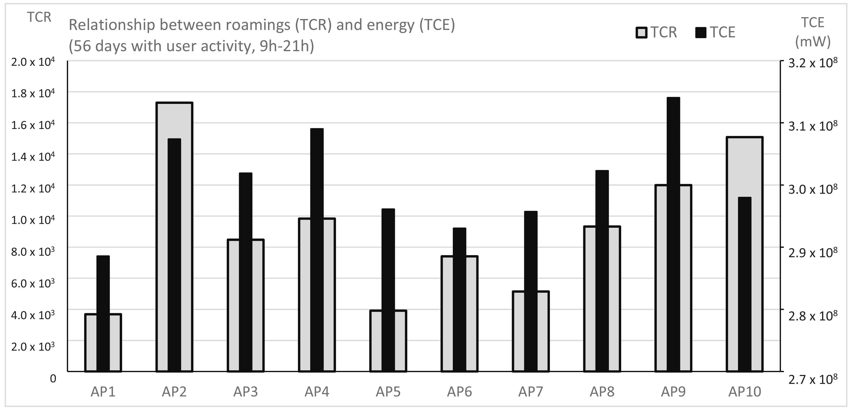
3.1. Current Network Status and Relationship between Energy and Roamings

We start from a full Wi-Fi infrastructure composed of a set of APs (left side of Figure 1). We collect two kinds of data along the time for a high number of network users: energy use in each AP, and number of roamings that users establish in them. From these data sets we build a matrix of roamings and an array of energies.

The matrix $CR$ (Current Roamings) is composed of S rows and I columns, where S is the number of network users and I is the number of access points. Each ${cr}_{s,i}$ in the matrix represents the number of roamings that user s has registered in the AP i during the period considered. From this matrix, we form the array $TCR$ (Total Current Roamings) with the sum of each column, that gives us the total number of roamings established in the corresponding AP.

The array $TCE$ (Total Current Energy) is composed of the total energy used in each AP along the period, which has a certain contribution of the users’ activity determined by the number of roamings.

We can establish a relationship between $TCR$ and $TCE$ or, in other words, between users’ activity and energy. A first approach to the energy impact in the APs due to the users’ activity would be to consider a function based on point coefficients. Thus, for each AP i there is a coefficient $C_i$ that connects proportionally the number of roamings ($TC{R}_i$) and energy ($TC{E}_i$), as we express in (1). This proportional function based on point coefficients allows us to make a reasonable prediction of the energy if the corresponding number of roamings in the AP changes.

$${TCE}_i=C_i{TCR}_i=C_i\sum _{s=1}^S{cr}_{s,i}$$

(1)

Finally, the longer spent collecting data and more network users, the higher the accuracy of the prediction model, because of the users’ habits are better registered by means of the number of roamings established in each AP.

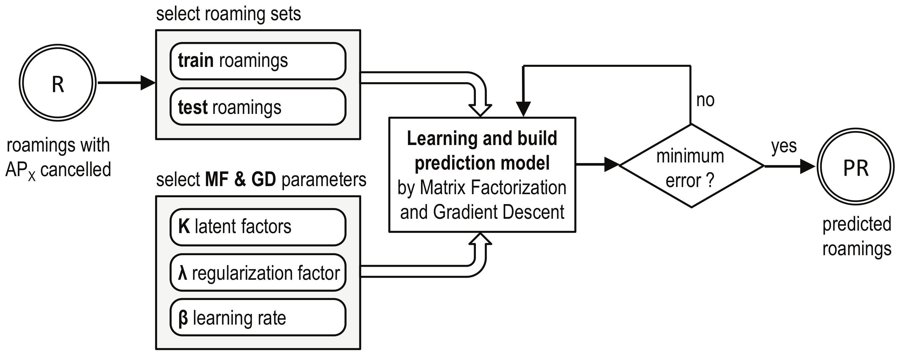
3.2. Predicting Roamings after Removing an Access Point

The removal of an AP can be due to several reasons, related to the infrastructure maintenance or planning. In this second phase of the energy prediction proposal (middle of Figure 1), we take advantage of a methodology inspired on RS and validated empirically, where the number of roamings can be predicted after removing an access point, as basis for a energy prediction in the simulated network.

The model starts from a matrix R (Roamings) built from $CR$ after performing two operations: First, we set to zero the roamings in the column corresponding to the AP removed. Second, we establish a set of cells ($D^{unk}$), distributed along the entire matrix following a particular strategy, as unknown values of roamings (they will be predicted), whereas the remaining cells are considered as known roamings ($D^{knw}$). In addition, we choose a set of training values as subset of known roamings ($D^{train}\subseteq D^{knw}$) to train the prediction model. This model will be more accurate if we consider a wider $D^{train}$, because it is built from more observed data. Last, we select a set of test roamings and also known values ($D^{test}\subseteq D^{knw}$), although usually much smaller than $D^{train}$, in order to validate the model by using the Root Mean Squared Error (RMSE) criterion (2).

$$RMSE=\sqrt{\frac{{\sum }_{s,i\in D^{test}}{(r_{s,i}-{\widehat{r}}_{s,i})}^2}{|D^{test}|}}$$

(2)

The prediction model considers Matrix Factorisation (MF). This technique approaches R to the product $W1W{2}^T$, where W1 and W2 are matrices of sizes ($S\times K$) and ($I\times K$) respectively. The s-th row $w{1}_s$ of $W1$ contains the K features that describe the user s and the i-th row $w{2}_i$ of $W2$ contains K corresponding features for the AP i. Then, the number of roamings $r_{s,i}$ given by the user s in the AP i is predicted as ${pr}_{s,i}$ according to (3), where k identifies the latent factor from 1 to K. Therefore, a new matrix $PR$ is built from R with the predicted values for the unknown roamings.

$${pr}_{s,i}=\sum _{k=1}^K\left(w{1}_{s,k}w{2}_{i,k}\right)={\left(W1W{2}^T\right)}_{s,i}$$

(3)

The methodology to predict the number of roamings by each user in each AP follows several steps as we can see in Figure 2. Initially, we select the train and test roaming datasets from R, and the main parameters for the learning phase (number of latent factors, learning rate and regularisation factor). Then, we define a prediction model in the learning phase by using MF, and learn it considering $D^{train}$ by using the algorithm Gradient Descent (GD) [21] in order to find the best values for W1 and W2. The optimal values are generated iteratively from the differences between real and predicted values. Once the model (both matrices) is obtained, we measure its goodness predicting the values of $D^{test}$ and calculating the difference with the real values by using the RMSE criterion. Last, all the values of the roaming matrix R are predicted from the optimal model found, in order to build the entire matrix $PR$.

Learning the model by GD means finding the optimal solutions W1 and W2, for a particular K. In this process, the initial solutions can be randomly chosen as positive real numbers generated from the normal distribution $N(0,{\sigma }^2)$ with standard deviation ${\sigma }^2=0.01$. Then, we calculate the difference $e_{s,i}$ (4) between real and predicted values in order to obtain the error (5).

$$e_{s,i}=p_{s,i}-{\widehat{p}}_{s,i}=p_{s,i}-\sum _{k=1}^K\left(w{1}_{s,k}w{2}_{i,k}\right)$$

(4)

$$err=\sum _{(s,i)\in D^{train}}{e}_{s,i}^2$$

(5)

This error is minimised updating W1 and W2 iteratively, which is very efficient in handling large datasets [22]. Gradient Descent needs to know, for each data, in which direction to update the values of $w{1}_{s,k}$ and $w{2}_{i,k}$. This can be known calculating the gradient of $e_{s,i}^2$ applied to $w{1}_{s,k}$ and $w{2}_{i,k}$ (6) and (7). After obtaining the gradient, we can update the values of $w{1}_{s,k}$ and $w{2}_{i,k}$ to $w{1}_{s,k}^{\prime }$ and $w{2}_{i,k}^{\prime }$ in the opposite direction to the gradient, according to Equations (8) and (9) respectively, where $\beta$ is the learning rate.

$$\frac{\partial }{\partial w{1}_{s,k}}{e}_{s,i}^2=-2e_{s,i}w{2}_{i,k}=-2(p_{s,i}-{\widehat{p}}_{s,i})w{2}_{i,k}$$

(6)

$$\frac{\partial }{\partial w{2}_{i,k}}{e}_{s,i}^2=-2e_{s,i}w{1}_{s,k}=-2(p_{s,i}-{\widehat{p}}_{s,i})w{1}_{s,k}$$

(7)

$$w{1}_{s,k}^{\prime }=w{1}_{s,k}-\beta \frac{\partial }{\partial w{1}_{s,k}}{e}_{s,i}^2=w{1}_{s,k}+2\beta e_{s,i}w{2}_{i,k}$$

(8)

$$w{2}_{i,k}^{\prime }=w{2}_{i,k}-\beta \frac{\partial }{\partial w{2}_{i,k}}{e}_{s,i}^2=w{2}_{i,k}+2\beta e_{s,i}w{1}_{s,k}$$

(9)

The iterative process ends when a stop criterion has been reached, for example, when a predefined number of iterations has been performed. Nevertheless, we choose a stop criterion when the error is greater or equal than the previous one, which means its minimum value has been reached; this provides higher accuracy, but could imply more computing effort in some cases.

In order to prevent large values of the factor vectors (over-fitting), we add a term to $e_{s,i}^2$ (10), where $\lambda$ is the regularisation term. Therefore, the newer gradients (11) and (12) update the values in W1 and W2 according to (13) and (14) respectively.

$$e_{s,i}^2={(p_{s,i}-{\widehat{p}}_{s,i})}^2+{\lambda \left(\right|\left|W1\right||}^2+{\left|\right|W2\left|\right|}^2)$$

(10)

$$\frac{\partial }{\partial w{1}_{s,k}}{e}_{s,i}^2=-2e_{s,i}w{2}_{i,k}+\lambda w{1}_{s,k}$$

(11)

$$\frac{\partial }{\partial w{2}_{i,k}}{e}_{s,i}^2=-2e_{s,i}w{1}_{s,k}+\lambda w{2}_{i,k}$$

(12)

$$w{1}_{s,k}^{\prime }=w{1}_{s,k}-\beta \frac{\partial }{\partial w{1}_{s,k}}{e}_{s,i}^2=w{1}_{s,k}+\beta (2e_{s,i}w{2}_{i,k}-\lambda w{1}_{s,k})$$

(13)

$$w{2}_{i,k}^{\prime }=w{2}_{i,k}-\beta \frac{\partial }{\partial w{2}_{i,k}}{e}_{s,i}^2=w{2}_{i,k}+\beta (2e_{s,i}w{1}_{s,k}-\lambda w{2}_{i,k})$$

(14)

The criterion RMSE applied on $D^{test}$ acts as a goodness measure of the model. Once W1 and W2 are obtained, the number of roamings performed by the user s in the AP i can be predicted by (3). The prediction is useful when we do not know the number of roamings (they have not been recorded) or for suggesting other APs according to the users’ behavior.

Lastly, we build a new array, $TPR$ (Total Predicted Roamings), composed of the I values where each of them (${TPR}_i$) represents the sum of the S roamings in $PR$ corresponding to ${AP}_i$. This array will be used in the next phase of the energy prediction proposal.

3.3. Energy Prediction for the Simulated Network

In the last phase of our proposal, we make a prediction of the energy used in the APs for the simulated network environment. The users’ activity that would be registered in the AP removed in the former network is now turned to other APs. The roamings prediction calculated in the second phase tried to answer to the question of what amount of the users’ activity has been taken by the other APs. Thus, this amount of roamings ($TPR$) should have the corresponding effect on the energy of the APs.

As we expect that the number of roamings has a proportional effect on the energy of the APs, we can export the relationship determined by the point coefficients $C_i$ in (1) during the first phase to the simulated environment, assuming the values of these coefficients remain constants. Consequently, we can build the array $TPE$ (Total Predicted Energy), where each element $TP{E}_i$ is given by (15) and represents the total energy predicted for the access point i.

$${TPE}_i=C_i{TPR}_i=C_i\sum _{s=1}^S{pr}_{s,i}$$

(15)

4. Experimental Environment

We consider a real wireless environment for collecting data for the experiments: two floors of the library building in the central campus of the University of Extremadura (UEX), Spain. This Wi-Fi network is composed of 10 access points accessed by a high number of users along the academic year.

4.1. Access Point Technology

The AP devices considered for the experiments were Alcatel-Lucent IAP-215 from Aruba Networks. They have dual radio $3\times 3$ MIMO technology and support standards 802.11ac at 1.3 Gbps in 5 GHz band and 802.11n at 450 Mbps in 2.4 Ghz band. The APs are focused on high-performance Wi-Fi environments with medium users’ density (up to 256 simultaneous users and 16 BSSIDs or Virtual APs per radio). The devices are configured as hive in Instant AP mode under InstantOS operating system from Aruba. At the same time, the hive is monitored by Nodowifi, a management tool from UEX.

The APs have 6 integrated omnidirectional downtilt antennae (3 per radio) with a maximum gain per antenna of 5 dBi. Nevertheless, the maximum gain of the antenna operating in the same band is 6.9 dBi at 2.4 Ghz and 8.8 dBi at 5 GHz. The power and channel assignment in the installed APs is driven by Adaptive Radio Management (ARM) technology from Aruba, which analyses the frequency spectrum in order to select the optimal power and channel, according to the regional configuration and the interferences and signals received from other devices. In any case, the power is selected in the range from 13 dBm to 18 dBm in both radios.

The IAP-215 device has a CPU Freescale P1010 800 MHz, 256 MB SDRAM and 32 MB flash memories. The processor has a 45 nm, low power single core e500, with 36-bit physical addressing, double-precision floating-point support, 32 KB L1 separated caches and 256 KB L2 cache, 3 Ethernet 10/100/1000 Mb/s enhanced ports, TCP/IP acceleration and classification capabilities, and integrated security engine supporting several crypto algorithms.

Lastly, the power of the APs is supplied by PoE (Power Over Ethernet) of 48 VDC with 802.3af compliance. The maximum operational energy consumption is 14.9 W, the minimum with radius is 4.5 W, and the power base emitting both radios at 18 dBm without connected users is 7 W. The efficiency of the PoE energy conversion to 12 VDC is around 88%.

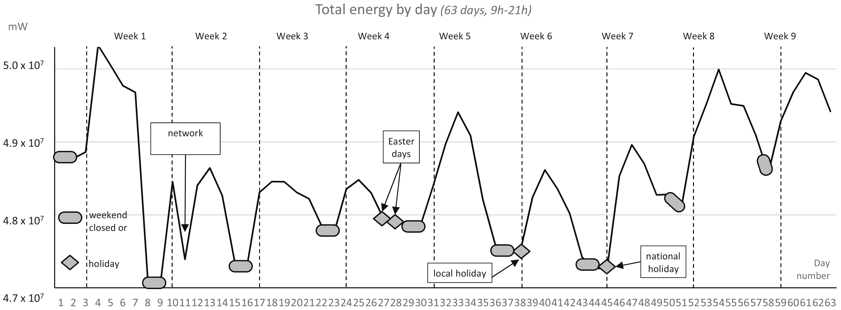
4.2. Collecting Data

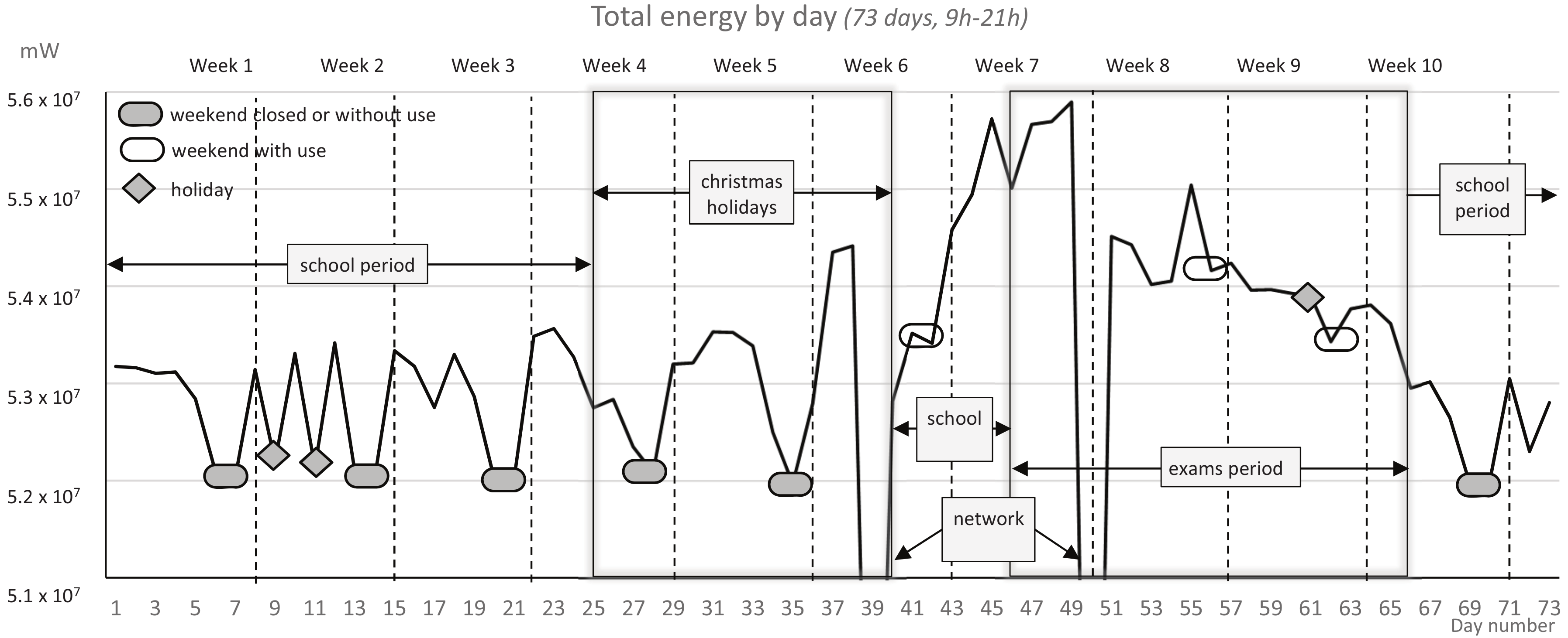
The energy and roaming data were collected via shell and stored in a table of a SQL database. In addition, we generated two different datasets according to two possible time slots to further analysis: full (24 h/day) or reduced time slot (12 h/day, corresponding to the interval from 9:00 to 21:00). The reason for considering a reduced time slot was to acquire a closer knowledge of the effect of the users’ behavior on the energy, since the usual activity of the network users is given during this time slot in the library building.

With regard to the energy use in each AP, we collected the data at regular intervals during an enough long period (we took into account that the network failed some hours in two days):

• Period: 73 days.
• Start time: 28 November 2016, at 00 h:00 m:01 s.
• End time: 8 February 2017, at 23 h:59 m:01 s.
• Sampling interval: 60 s.
• Total energy measures collected: 1,048,240 samples = 104,824 samples by AP.

With regard to the number of roamings registered in each AP during the same period, we know the corresponding number to each network user: 2937 users considering all day (24 h/day) and 2907 users considering the range 9 h to 21 h (12 h/day).

Another possibility to collect the roaming data was to map roamings with MAC addresses instead of user identifications. Nevertheless, we decided to go with identifications since they reflect the users’ behaviour better: the same user can access the AP using different devices (laptops, smartphones), so we can obtain roaming registers from different MACs that correspond with the same user. In addition, we considered the number of roamings instead of traffic data because we pursuit to reflect the users’ behavior regarding the use of the network infrastructure instead of reflecting elements outside of the AP demand, as this could be the types and characteristics of the communication content.

When there is not a login due to a failed connection, the database registers it under a special user identification, so we exclude this data. Besides, we exclude another special user that identifies the connection of external users through anonymous logins using tunnels.

5. Data Analysis

Before predicting the energy in a Wi-Fi network where an access point was removed, it is important to analyse the current network infrastructure in order to decide some aspects for building the prediction model. For example, we should exclude some days where the characteristics of the data collected could lead to a misinterpretation of the prediction results, as we go on to explain.

5.1. Total Energy Used in the Access Points in the Period

Figure 3 shows the daily evolution of the total energy of the APs during the period, although we only consider the time slot of interest (12 h daily, from 9:00 to 21:00).

We can distinguish some periods in the full period of 73 days, where the effects of the users’ behaviour on the energy were different. First, there is a 16-day period corresponding with the Christmas holidays; in this period, the library was open for many days (8), although the network failed during one of them. The proximity of the exam period favoured regular user activity during this period. In addition, the library closed for 3 holidays and 6 weekends (some of which included these holidays). The roamings data corresponding to these days were not considered for generating the prediction model, because they do not represent users’ activity; the energy data is only represented by regular operations of the access points.

Besides, there were four weekends where the library opened in order to allow students to prepare for their exams; we considered the roaming and energy data of these weekends within the prediction model. Also, the library remained opened during the exam period with a great users’ activity, because of a number of students higher than ordinary days. This had a corresponding effect on the energy use. These days, together with two school periods (ordinary days), are suitable for the prediction model. Lastly, there were two days where the network was unavailable. The data registered were not roamings, but energy; since this energy was due only to normal operations excluding the users’ impact, we have not considered these two days in order to avoid an significant distortion in the prediction model.

In view of the above considerations, we set a period of 56 days to elaborate the prediction model. This period corresponds with the full period of 73 days excluding 2 days with the network unavailable; 12 days on weekends and 3 holidays. The resulting days include two school periods and the exam period, as well as some days over the Christmas holidays while the library was open.

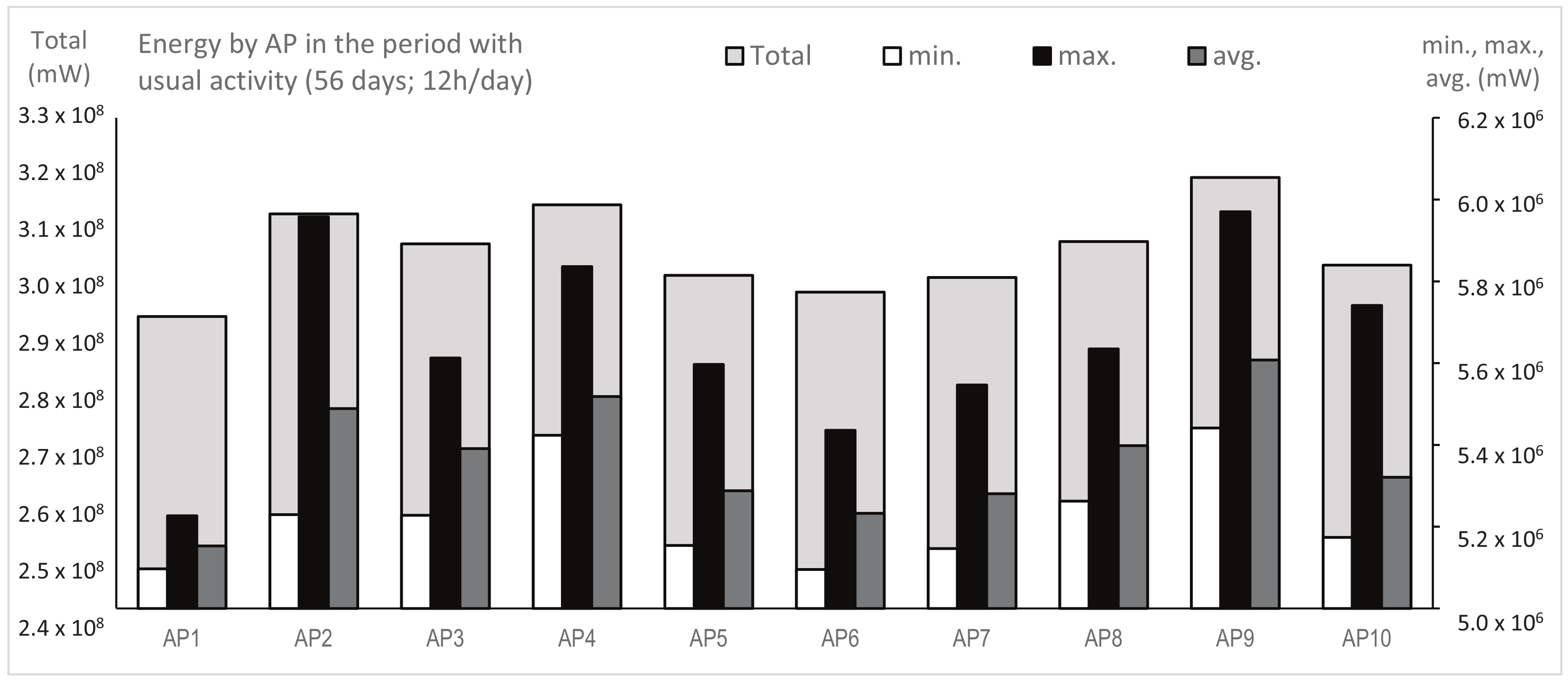
5.2. Energy Use by AP in the Period

Figure 4 shows the minimum, maximum, average and total energy in each AP, considering the valid period (56 days with users’ activity) and the usual time slot (9:00 to 21:00). We can see $A{P}_9$ and $A{P}_1$ used more and less energy respectively, whereas $A{P}_8$ is at a middle level; this is the reason why we chose $A{P}_8$ to be removed from the network in order to make the roaming and energy prediction.

Out of the time slot of interest, we know the minimum energy (from 4 to 4.8 W) is reached around 5:00, when the APs reboot following a programmed schedule. Once the radios start, and according to the assigned power (from 13 dBm to 18 dBm), the energy use climbs to 7 W approximately.

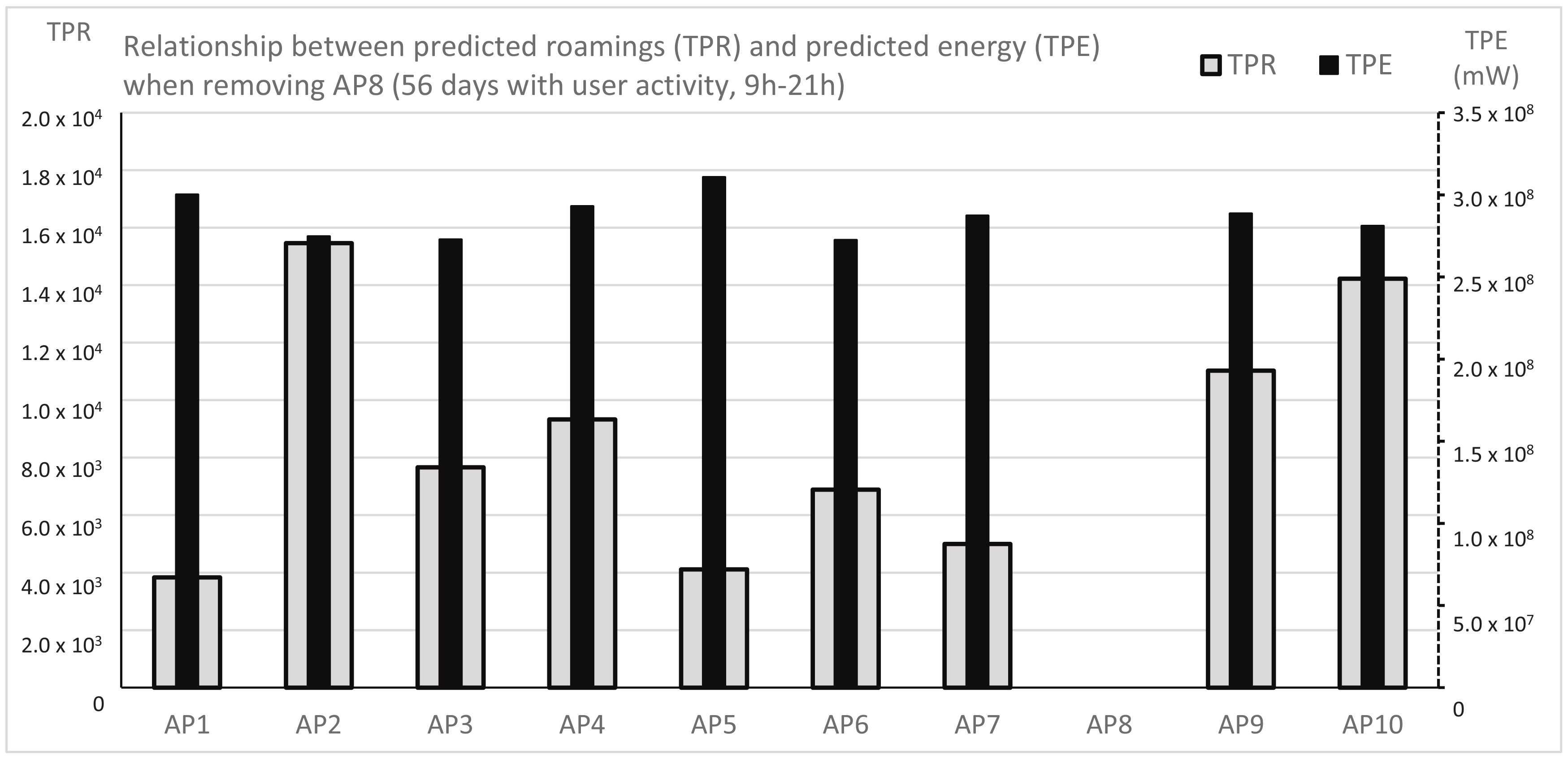
6. Energy Prediction

In this section, we present the results of the energy and roamings prediction of the network after removing $A{P}_8$, following the three phases described in Section 3.

First, we analyse the full network infrastructure during the valid period (56 days, time slot 9:00–21:00) from the collected data and the relationship between roamings and energy. After obtaining the total energy measured in each AP as the array $TCE$, the number of roamings by user in each AP as the matrix $CR$, and the total roamings by AP as the array $TCR$, we calculate the coefficients array C according to (1). These coefficients represent the effect of the users’ behaviour (expressed as the number of roamings) on the energy used in the APs. This effect is unique for each AP, because of their particular characteristics (placement, level of interferences, wire lengths, etc.), hence the point relationship.

Figure 5 shows graphically the proportional point relationship between energy (bars $TCE$) and roamings (bars $TCR$) in the APs during the period for the full network infrastructure. This relationship is given by the coefficients C.

Secondly, we bring up a simulated network removing $A{P}_8$. First, we build R from $CR$ setting to zero the roamings corresponding to $A{P}_8$. At the same time, we select the unknown values in $CR$ according to a strategy where we select just one cell by row as an unknown value, following successive column positions; this guarantees enough representation in the matrix to force the learning algorithm to consider varied characteristics of users and access points, as it was validated in [20]. Next, we elaborate the prediction model defined by W1 and W2, both calculated using MF and GD, according to their main parameters: training and test datasets, latent factors, the learning rate and the regularisation term.

The values for these parameters were chosen carefully, according to the characteristics of the prediction context (nature of the problem, size of the training dataset, etc.), since certain values can be good in some contexts and worse in others. K has to do with the factors related to the network context and users’ behavior; it is not known and is difficult to identify, although it might be not very high. The convergence of GD is affected by the value of $\beta$; although the most usual case is to select a fixed value, it also can be adjusted automatically (if the algorithm does not converge or for accelerating the convergence) or adaptively selected [23,24]. Last, $\lambda$ could affect the accuracy of the prediction error, although it can be chosen from a wide range of values with no worries. For these reasons, we ran many prediction experiments in a similar context (prediction of roamings in a larger Wi-Fi network), considering different values of K, $\beta$ and $\lambda$ [20]. Specifically, the experiments for choosing the best K considered a large network composed of 37 APs and 1517 users collecting roamings during 30 days, and they selected K values from 2 to 100. After calculating the corresponding predictions, we observed that higher K values caused worse predictions. As the factorization models are implicitly able to encode latent factors of users and APs, the intuition behind using MF is that there should be some latent features that determine how a user interacts an AP. The experiments done reported good predictions for K = 4, so these factors could be, apart from typical success login and wrong login, connection time and signal strength, for example. With regard to $\beta$ and $\lambda$, we ran a set of experiments in the similar context considering the same values for both them: 100, 75, 50, 25, 10, 5, 2.5, 1, 0.5, 0.1, 0.05, 0.01, and 0.005. We found out that the pair {$\beta$ = 1, $\lambda$ = 75} reported the minimum prediction error.

Once we obtained the optimal prediction model, we generated the matrix $PR$ which contains the predicted number of roamings for the simulated network, as we can see in Figure 6. From matrix $PR$, we obtained the array $TPR$ with the total number of predicted roamings for each AP. Obviously, the corresponding value of $TPR$ for $A{P}_8$ is zero.

In the last phase, we calculated the predicted energy in the simulated network, storing it in the array $TPE$. These values were calculated from the array $TPR$ and the point coefficients C obtained in the first phase, according to (15). Figure 6 shows the array $TPE$ with the predicted energy, which was the main goal of our research proposal.

7. Experimental Validation

Figure 1 includes a work phase for the experimental validation of the proposed prediction method. The validation comes from collecting new energy and roaming data in the same wireless network where $A{P}_8$ was really removed. Obviously, the corresponding new period is different to the one considered for the prediction works, because it is later and can have a different number of days. However, this circumstance does not impede the validation works for two reasons. On the one hand, the users’ behaviour is supposed to be similar in two different periods when both consider enough working days in the same academic environment; on the other hand, the users’ behaviour is responsible for the roaming distribution among the different access points of the network, with the corresponding effect in their energy consumption.

The experimental validation starts by removing $A{P}_8$ from the wireless network, not in a simulation mode as in the prediction, but in reality. The resulting network is called the “new network” from this point onwards. Next, we collect roaming and energy data in the access points during a determined period. Once we stop collecting data, we can calculate the relationship between roamings and energy for the new network. Finally, we compare the energy distribution among the access points of the new and simulated networks for a qualitative validation of the prediction method proposed.

Figure 7 shows the period considered for collecting data in the new network. It consists of 63 days, 40 of which were working days with usual academic activity, useful for comparison purposes (the building was closed for 22 days and the network failed one day). As in the prediction works, we filter the collected data for the daily time slot reduced (12 h, from 9:00 to 21:00), because the usual network demand takes place in that slot. The new period considers the activity of 3083 users.

We build three datasets from the collected data:

• $NR$ (“New Roamings”). It is a $S\times I$ matrix, where S is the number of users ($S=3083$) and I is the number of APs ($I=10$). The cell $n{r}_{s,i}$ is the number of total roamings due to user s in the AP i during the entire period. As $A{P}_8$ was removed, the entire column $i=8$ is set to zero in the matrix.
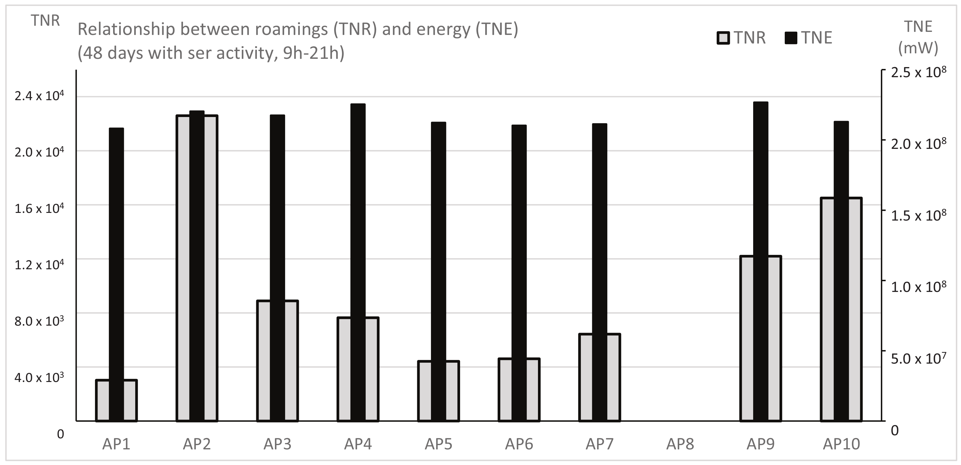
• $TNR$ (“Total New Roamings”). It is an array of size I where $TN{R}_i$ is the number of roamings stablished in the AP i by all the users during the period. This value is calculated by adding the entire column i in $NR$.
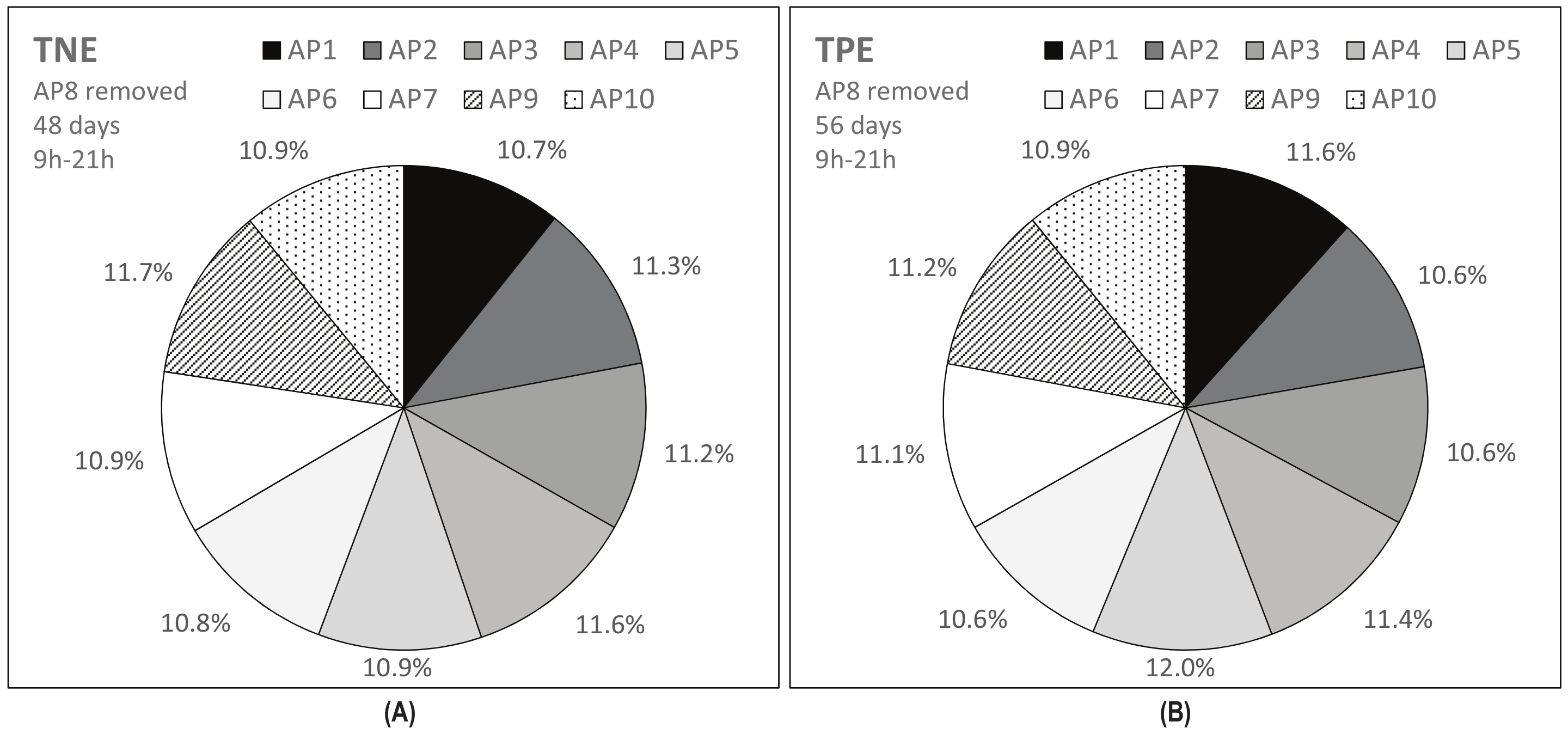
• $TNE$ (“Total New Energy”). It is an array of size I where $TN{E}_i$ is the total energy in the AP i in the period. As in the prediction, the energy values in this array are filtered to consider only the period (40 days) where the network was available for the users. Therefore, we assure these energy values show the users’ behaviour.

We can calculate the relationship between users’ activity ($TNR$) and energy consumption in the access points ($TNE$) by means of point coefficients $C{N}_i$ (16), following a similar formula as for the prediction process. The link between both datasets is reasonable because the roamings were generated during the days when the network was available for the users, which are the same days taken into account to calculate the array $TNE$.

$${TNE}_i=C{N}_i{TNR}_i=C{N}_i\sum _{s=1}^S{cnr}_{s,i}$$

(16)

The experimental validation of the prediction proposal comes from the comparison between the $TPE$ and the $TNE$ datasets. The first dataset contains the energy predicted in the APs of the simulated network during the first period; these energies were obtained applying the prediction model to the entire network using $TCR$ (roamings) and $TCE$ (energies). The second dataset contains the energy in the APs of the new network during the second period. From the $TPE$ and the $TNE$ we calculate, for the two periods considered, the energy rates in each AP due to users’ behaviour. Hence, the comparison among the corresponding rates checks the validity of the prediction model, because the users’ behavior is similar in periods with the same characteristics of network availability and use when the same AP is removed. We can say that the experimental validation is successful if the energy distribution among the access points is similar in both periods, because the rates represent the energy contribution in each AP due to users’ behaviour.

Figure 8 shows the energy distribution among the access points when we remove $A{P}_8$. The graph on the left side (A) corresponds with the simulated network obtained from the prediction model, whereas the right side (B) shows the distribution in the new network. We can check that the rates are very similar in both cases, confirming the validity of the prediction method proposed under a qualitative point of view. More accurate results could be obtained just using optimal learning rate and regularisation factor, different training datasets, and new point coefficients formula, among other possibilities.

We can show an additional qualitative validation comparing the relationships between roamings and energies in the network without $A{P}_8$. Figure 6 shows how predicted roamings ($TPR$) and predicted energy ($TPE$) in the simulated network are related between them through point coefficients $C_i$ (1). In the same way, Figure 9 shows the link between roamings ($TNR$) and energy ($TNE$) in the new network through point coefficients $C{N}_i$ (16).

Both figures can be compared under a qualitative point of view, because the periods for collecting data in full and new networks are different. Comparing the corresponding columns in both figures for each access point, we can check that they keep similar proportions, which adds another support to the validity of the prediction proposal.

8. Discussion

Figure 6 allows us to know the amount of energy in each access point that increases or decreases after removing $A{P}_8$ in the Wi-Fi network, as we can see in Figure 10. This information is very useful for planning maintenance tasks in the network infrastructure. Of course, we can apply this methodology to any access point, repeating the calculations accordingly for the simulated environment.

It is important to emphasize that the relationship between predicted roamings and energy is based on coefficients obtained from real data. This guarantees that each point coefficient takes into account the particular characteristics of the corresponding access point (wire length, transmission power, interferences, etc.). These particular and different characteristics of each access point explains how we observe higher energies in some cases where the number of roamings is smaller, and vice versa. Consequently, our energy prediction proposal has the advantage of being based not on theoretical constructions, but on experimental frameworks that take into account the particular factors of each wireless infrastructure.

Future works can improve our proposal. In this sense, we plan to validate the prediction method by checking the effect of cancelling other access points different to $A{P}_8$ (considering enough period size) and considering other wireless infrastructures and environments where users reflect other behaviours. Besides, we would like to go more deeply into the relationship between roamings and energy, extending the point coefficients formula to obtain a more accurate one and considering smaller sampling periods for collecting energy data.

References

1. Petroski, J. Power over Ethernet thermal analysis with an engineering mechanics approach. In Proceedings of the 2016 32nd Thermal Measurement, Modeling Management Symposium (SEMI-THERM), San Jose, CA, USA, 14–17 March 2016; pp. 50–56. [Google Scholar]
2. Jannach, D.; Zanker, M.; Friedrich, G. Recommender Systems: An Introduction; Cambridge University Press: Cambridge, UK, 2011. [Google Scholar]
3. Hamamoto, R.; Takano, C.; Obata, H.; Aida, M.; Ishida, K. Setting Radio Transmission Range Using Target Problem to Improve Communication Reachability and Power Saving. In Ad Hoc Networks, Proceedings of the 7th International Conference (AdHocHets 2015), San Remo, Italy, 1–2 September 2015; Mitton, N., Kantarci, M.E., Gallais, A., Papavassiliou, S., Eds.; Springer: Cham, Switzerland, 2015; pp. 15–28. [Google Scholar]
4. Konstantinidis, A.; Yang, K. Multi-objective K-connected Deployment and Power Assignment in WSNs using a problem-specific constrained evolutionary algorithm based on decomposition. Comput. Commun. 2011, 34, 83–98. [Google Scholar] [CrossRef]
5. Venckauskas, A.; Jusas, N.; Kazanavicius, E.; Stuikys, V. Identification of Dependency among Energy Consumption and Wi-Fi Protocol Security Levels within the Prototype Module for the IoT. Elektron. Elektrotech. 2014, 20, 132–135. [Google Scholar]
6. Zhang, H.; Chu, X.; Guo, W.; Wang, S. Coexistence of Wi-Fi and heterogeneous small cell networks sharing unlicensed spectrum. IEEE Commun. Mag. 2015, 53, 158–164. [Google Scholar] [CrossRef]
7. He, H.; Shan, H.; Huang, A.; Cai, L.X.; Quek, T. Proportional Fairness-Based Resource Allocation for LTE-U Coexisting with Wi-Fi. IEEE Access 2016, 5, 4720–4731. [Google Scholar] [CrossRef]
8. Shen, Y.; Jiang, C.; Quek, T.Q.S.; Zhang, H.; Ren, Y. Pricing equilibrium for data redistribution market in wireless networks with matching methodology. In Proceedings of the 2015 IEEE International Conference on Communications (ICC), London, UK, 8–12 June 2015; pp. 3051–3056. [Google Scholar]
9. Scellato, S.; Musolesi, M.; Mascolo, C.; Latora, V.; Campbell, A.T. NextPlace: A Spatio-temporal Prediction Framework for Pervasive Systems. In Pervasive Computing, Proceedings of the 9th International Conference (Pervasive 2011), San Francisco, CA, USA, 12–15 June 2011; Lyons, K., Hightower, J., Huang, E.M., Eds.; Springer: Berlin/Heidelberg, Germany, 2011; pp. 152–169. [Google Scholar]
10. Hamamoto, R.; Takano, C.; Obata, H.; Ishida, K. Improvement of Throughput Prediction Method for Access Point in Multi-rate WLANs Considering Media Access Control and Frame Collision. In Proceedings of the 2015 Third International Symposium on Computing and Networking (CANDAR), Sapporo, Japan, 8–11 December 2015; pp. 227–233. [Google Scholar]
11. Dai, L.; Xue, Y.; Chang, B.; Cao, Y.; Cui, Y. Integrating Traffic Estimation and Routing Optimization for Multi-Radio Multi-Channel Wireless Mesh Networks. In Proceedings of the 27th Conference on Computer Communications (INFOCOM 2008), Phoenix, AZ, USA, 13–18 April 2008. [Google Scholar]
12. Baker, T.; Al-Dawsari, B.; Tawfik, H.; Reid, D.; Ngoko, Y. GreeDi: An energy efficient routing algorithm for big data on cloud. Ad Hoc Netw. 2015, 35, 83–96. [Google Scholar] [CrossRef]
13. Baker, T.; Ngoko, Y.; Tolosana-Calasanz, R.; Rana, O.F.; Randles, M. Energy Efficient Cloud Computing Environment via Autonomic Meta-director Framework. In Proceedings of the 2013 Sixth International Conference on Developments in eSystems Engineering, Abu Dhabi, UAE, 16–18 December 2013; pp. 198–203. [Google Scholar]
14. François, J.M.; Leduc, G. AP and MN-Centric Mobility Prediction: A Comparative Study Based on Wireless Traces. In NETWORKING 2007. Ad Hoc and Sensor Networks, Wireless Networks, Next Generation Internet: 6th International IFIP-TC6 Networking Conference, Atlanta, GA, USA, 14–18 May 2007, Proceedings; Akyildiz, I.F., Sivakumar, R., Ekici, E., Oliveira, J.C.D., McNair, J., Eds.; Springer: Berlin/Heidelberg, Germany, 2007; pp. 322–332. [Google Scholar]
15. Gmach, D.; Rolia, J.; Cherkasova, L.; Kemper, A. Workload Analysis and Demand Prediction of Enterprise Data Center Applications. In Proceedings of the 2007 IEEE 10th International Symposium on Workload Characterization, Boston, MA, USA, 27–29 September 2007; IEEE Computer Society: Washington, DC, USA, 2007; pp. 171–180. [Google Scholar]
16. Ghosh, A.; Jana, R.; Ramaswami, V.; Rowland, J.; Shankaranarayanan, N.K. Modeling and characterization of large-scale Wi-Fi traffic in public hot-spots. In Proceedings of the 2011 IEEE INFOCOM, Shanghai, China, 10–15 April 2011; pp. 2921–2929. [Google Scholar]
17. Duggan, J.; Chi, Y.; Hacigumus, H.; Zhu, S.; Cetintemel, U. Packing light: Portable workload performance prediction for the cloud. In Proceedings of the International Conference on Data Engineering, Brisbane, Australia, 8–12 April 2013; pp. 258–265. [Google Scholar]
18. Younis, M.; Akkaya, K. Strategies and techniques for node placement in wireless sensor networks—A survey. Ad Hoc Netw. 2008, 6, 621–655. [Google Scholar] [CrossRef]
19. Vilovic, I.; Burum, N. Location Optimization of WLAN Access Points Based on a Neural Network Model and Evolutionary Algorithms. J. Control Meas. Electron. Comput. Commun. 2014, 55, 317–329. [Google Scholar] [CrossRef]
20. Rodriguez-Lozano, D.; Gomez-Pulido, J.; Lanza-Gutierrez, J.; Duran-Dominguez, A.; Fernandez-Diaz, R. Context-aware prediction of access points demand in Wi-Fi networks. Comput. Netw. 2017, 117, 52–61. [Google Scholar] [CrossRef]
21. Koren, Y.; Bell, R.; Volinsky, C. Matrix Factorization Techniques for Recommender Systems. Computer 2009, 42, 30–37. [Google Scholar] [CrossRef]
22. Bottou, L. Large-Scale Machine Learning with Stochastic Gradient Descent. In Proceedings of the 19th International Conference on Computational Statistics, Paris, France, 22–27 August 2010; Springer: Heidelberg, Germany, 2010; pp. 177–186. [Google Scholar]
23. Zhang, R.; Gong, W.; Grzeda, V.; Yaworski, A.; Greenspan, M. An Adaptive Learning Rate Method for Improving Adaptability of Background Models. IEEE Signal Process. Lett. 2013, 20, 1266–1269. [Google Scholar] [CrossRef]
24. Ranganath, R.; Wang, C.; Blei, D.M.; Xing, E.P. An Adaptive Learning Rate for Stochastic Variational Inference. In Proceedings of the 30th International Conference on Machine Learning, Atlanta, GA, USA, 17–19 June 2013; pp. 1–9. [Google Scholar]
Figure 1. Methodology for predicting the energy in the access points after removing one of them.
Applsci 07 00825 g001
Figure 2. Methodology to generate a prediction model from Matrix Factorisation and Gradient Descent. This model will predict the number of roamings in each AP produced by each user considering a Wi-Fi infrastructure where a particular AP has been cancelled.
Applsci 07 00825 g002
Figure 3. Daily evolution of the energy of the access points in the period, considering the time slot from 9:00 to 21:00.
Applsci 07 00825 g003
Figure 4. Minimum, maximum, average and total energy in each AP, considering the valid period (56 days with users’ activity) and the usual time slot (9:00 to 21:00).
Applsci 07 00825 g004
Figure 5. Proportional point relationship between energy ( T C E ) and roamings ( T C R ) in the APs during the period for the full network, given by the coefficients C.
Applsci 07 00825 g005
Figure 6. Energy prediction ( T P E ) in the simulated network, obtained from the roamings predicted ( T P R ) considering the same point coefficients C that define the relationship between roamings and energy for the full network.
Applsci 07 00825 g006
Figure 7. Daily evolution of the energy of the access points in the new period for validation purposes, considering the time slot from 9:00 to 21:00.
Applsci 07 00825 g007
Figure 8. Energy distribution among the APs in the simulated network (A) and new network (B).
Applsci 07 00825 g008
Figure 9. Proportional point relationship between energy ( T N E ) and roamings ( T P R ) in the APs during the period for the new network, given by the coefficients C N .
Applsci 07 00825 g009
Figure 10. Increase of the energy in the APs after removing A P 8 .
Applsci 07 00825 g010