1. Introduction
The automobile industry is immensely working to transform conventional road vehicles into partial/full autonomous vehicles. SAE International and NHTSA have classified six levels of driving autonomy from “no automation” to “full automation” [
1,
2]. In particular, from the lane-keeping assistance system [
3] to fully automated maneuvering [
4,
5,
6], Steer-by-Wire (SbW) technology is playing a fundamental role in advanced driving assistance systems [
7]. Nissan introduced the first commercialized SbW system in 2013 with the Infiniti Q50 vehicle [
8,
9]. The SbW system delivers better overall steering performance with comfort, reduces power consumption, provides active steering control, and significantly improves the passenger safety. Compared with a conventional steering system, the SbW system has replaced the mechanical shaft between the steering wheel and front wheels with two actuators, controllers, and sensors. The first actuator steers the front wheels and the second actuator provides steering feel feedback to the driver, obtained from the road and tire dynamics.
Over the last decade, many researchers have proposed a number of control techniques to compensate for the system parameter variation, change in road conditions, and external disturbances for obtaining the robust performance of the SbW system. In [
10,
11], sliding mode based control schemes are proposed for a partially known SbW system with unknown lumped uncertainties to track the reference signal. However, it is hard to classify the wide range of nominal parameters under the sideslip, and the robust performance may not be guaranteed over different road conditions. In [
12,
13,
14,
15,
16], the upper bound sliding mode control (SMC) technique is proposed for the bounded unknown SbW system parameters and uncertain dynamics. However, the process of obtaining these proper bounds is not evident. In [
17,
18,
19,
20] proportional-derivative (PD) control is proposed to follow the driver’s steering wheel signal closely. However, under uncertain dynamics, it is difficult to achieve satisfactory performance with a conventional control scheme. In [
21] cornering stiffness and chassis side slip angle are estimated to calculate the self-aligning torque. The authors used the proportion of estimated torque as a feedback to the driver for artificial steering feel. In [
22] three suboptimal sliding mode techniques are evaluated for yaw-rate tracking problem in over-actuated vehicles. In [
23,
24], adaptive control is implemented for path tracking via SbW system and the authors estimated the sliding gains by considering the known steering parameters and cornering coefficients. However, they did not use any mechanism to stop the estimation. Consequently, the controller could lead to saturation by estimating too large a sliding gain. In [
25,
26] the authors proposed a hyperbolic tangent function with adaptive SMC based schemes to counter the effect of self-aligning torque. In [
27] the frictional torque and self-aligning torque are replaced by a second-order polynomial function that acts as an external disturbance over the SbW system. The authors proposed an adaptive terminal SMC (ATSMC) to estimate the upper bounds of parameters and disturbance.
Apart from the control design, a robust estimation methodology is also needed for the SbW system to estimate the vehicle states, uncertain parameters, and tire–road conditions for eliminating the effect of external disturbances from the controller. For instance, in recent years Kalman filter (KF) and nonlinear observers have gained much more attention from researchers; for example, in [
28] a dual extended KF is used to estimate vehicle states and road friction. In [
29] the authors estimated five DOF vehicle states and inertial parameters, such as overloaded vehicle’s additional mass, respective yaw moment of inertia, and its longitudinal position using the dual unscented KF by considering the constant road–tire friction over a flat road. In [
30,
31,
32] a fixed gain based full-state nonlinear observer is designed to estimate the longitudinal, lateral, and yaw velocities of the vehicle. However, for good estimation performance the observer gains must be tuned to a wide range of driving conditions. In order to reduce the burden of gain tuning from a-nonlinear observer [
33], employed linear matrix inequality based convex optimization to obtain the gains of reduced order observer for estimating vehicle velocities. In [
34] the authors implemented an adaptive gain based sliding mode observer to estimate the battery’s charging level and health in electric vehicles.
In this paper first, we have established the adaptive sliding mode observer (ASMO) and the Kalman filter (KF) to simultaneously estimate the vehicle states and cornering stiffness coefficients by using the yaw rate and the strap down [
35] lateral acceleration signals. Then, based on the simultaneously estimated dynamics, the two-fold adaptive global fast sliding mode control (AGFSMC) is designed for SbW system vehicles, considering that the steering parameters are unknown. In the first fold, estimated dynamics-based control (EDC) is utilized to stabilize the impact of self-aligning torque and frictional torque. In the second fold, the AGFSMC is developed to estimate the uncertain SbW parameters and eliminate the effect of residual disturbance left out from the EDC. The adaptation capability of the proposed scheme not only intelligently handles the tire–road environmental changes, but also adapts the system parameters and sliding gains according to the different driving conditions.
Finally, for avoiding overestimations of parameters and gains, discontinuous projection mapping [
36] is incorporated to stop the estimation and adaptive mechanism as the tracking error converges to the designed dead zone bounds [
37]. In the simulated results section, the comparative study will show the effectiveness of the proposed AGFSMC scheme, which ensures that the tracking error and sliding surface converge asymptotically to zero in a finite time.
The rest of the paper is structured as follows: In
Section 2 and
Section 3, vehicle dynamics modeling and SbW system modeling with external disturbance are discussed. In
Section 4, the ASMO and KF are established to estimate the vehicle states and parameters. In
Section 5, the AGFSMC scheme is developed for the SbW system and the convergence analysis with bounded conditions is discussed in detail.
Section 6 describes the simulation results and findings to validate the proposed scheme, followed by the last section that concludes the paper.
2. Vehicle Dynamics Modeling
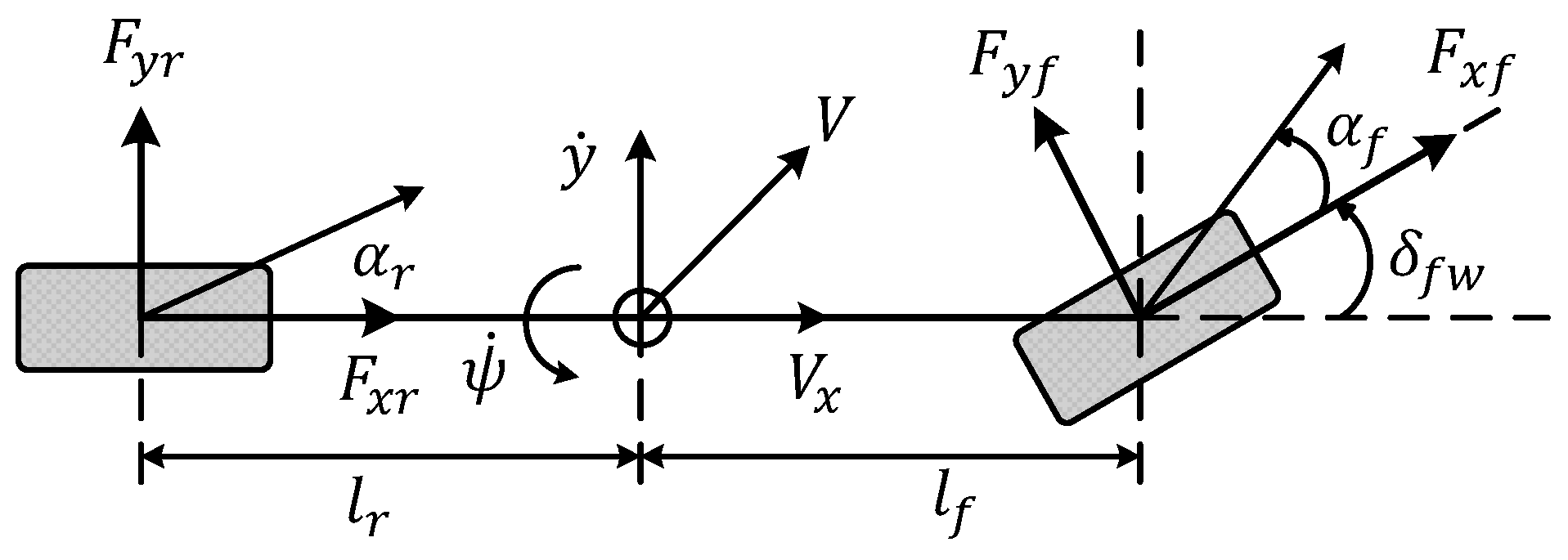
Figure 1 illustrates the simplest bicycle model of a vehicle, which has a central front wheel and a central rear wheel, in place of two front and two rear wheels. The vehicle has two degrees of freedom, represented by the lateral motion
and the yaw angle
. According to
Figure 1, the dynamics along the
axis and yaw axis are described as [
38,
39]:
where
, and
. are the acceleration with respect to the
axis motion, yaw rate, and yaw acceleration, respectively.
and
represent the distance of front and rear axles from the center of gravity, respectively.
and
are the mass of vehicle and the moment of inertia along the yaw axis, respectively.
denotes the longitudinal vehicle velocity at the center of gravity.
and
are the longitudinal forces of the front and rear wheels, respectively.
and
are the lateral frictional forces of front and rear wheels, respectively, as shown in
Figure 1.
In order to simplify the model, it is assumed that longitudinal forces
are equal to zero and by using the small angle approximation, i.e.,
, the simplified dynamics can be modeled as follows:
For small slip angles, the lateral frictional forces are proportional to slip-angle
and
at the front and rear wheels, respectively. Therefore, lateral forces are defined as:
where
where
and
are the front and rear tires’ cornering stiffness coefficients.
denotes the steering angle of front wheels, which is considered the same for both front wheels, and factor
accounts for two front and two rear wheels, respectively.
By using the small angle approximation
[
38], Equations (7) and (8) can be written as:
Substituting Equations (5), (6), (9) and (10) into Equations (3) and (4), the state space model is represented as:
where
3. Steer-by-Wire System Modeling
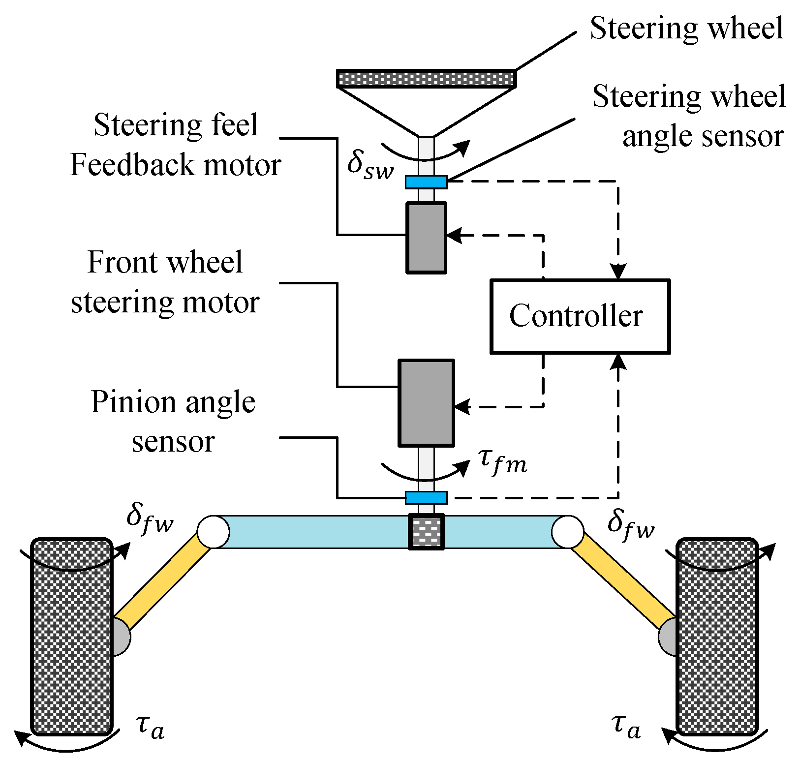
Figure 2 depicts the standard model of SbW system for road vehicles. As shown, the steering wheel angle sensor is used to detect the driver’s reference angle and the feedback motor is used to provide the artificial steering feel.
Similarly, the front wheel angle is detected by the pinion angle sensor. Based on the error between the reference angle and the front wheel angle, the control signal is provided to the front wheel steering motor to closely steer the front wheels according to the driver’s reference angle.
The equivalent second-order dynamics of the front wheels’ steering motor is expressed as follows [
10,
15]:
where
and
are the equivalent moment of inertia and the equivalent damping of the SbW system, respectively.
is the front wheels’ steering motor control input and
is the steering ratio between the steering wheel angle and the front wheels’ angle, given by
.
It is known that many modern road vehicles use the variable steering ratio. Therefore, dividing both sides of Equation (13) by
eliminates the impact of the variable steering ratio from the proposed control scheme without compromising the steering performance. Thus, the dynamics of SbW system can be written as:
where
where
and
are the moment of inertia of the front wheels and the front wheel steering motor, respectively.
and
are the damping factors of the front wheels and the front wheel steering motor, respectively.
When the vehicle is turning, the steering system experiences torque that tends to resist the attempted turn, known as self-aligning torque
. It can be seen from
Figure 3 that the resultant lateral force developed by the tire manifests the self-aligning torque. The lateral force is acting behind the tire center on the ground plane and tries to align the wheel plane with the direction of wheel travel. Therefore, the total self-aligning torque is given by [
14]:
where
is the pneumatic trail (the distance between the application point of lateral force
to the center of tire),
is the mechanical trail, also known as the caster offset, which is the distance between the tire center and the point where the steering axis intersects with the ground plane.
By substituting Equations (5) and (9) into Equation (19),
can be written as:
Moreover,
is the coulomb frictional torque acting on SbW system, expressed as [
23]:
where
is the normal load on front axle,
is the coeffient of friction,
is the vehicle’s weight without any external load, and
signum function is used to identify the direction of the frictional torque.
The stability of the SbW system mainly depends on the road and environmental conditions. The uncertain road surface such as dry, wet, or icy can produce considerable variations in the tire cornering stiffness coefficients , which can adversely affect the controller performance. Therefore, to estimate the vehicle states and the uncertain parameter variation, the cooperative ASMO and KF are designed in the next section.
4. ASMO and KF
In this section, we will first design the ASMO for yaw rate and lateral velocity , and then use the KF parameter estimator to estimate the tire cornering stiffness coefficients under varying road conditions.
In order to design the observer, a few assumptions are made, such as: the yaw rate
is directly measurable from yaw rate sensor; and the vehicle’s longitudinal velocity is obtained from
, where
is the effective tire radius and
is the averaged free wheels angular speed measured from the wheel encoders. Moreover, it is considered that there is no effect of gravitation acceleration
on the lateral acceleration
, such that the
measurement model is defined as [
29]:
Therefore, the lateral velocity can be obtained from a strapdown algorithm [
35] as follows:
where
is the prior lateral velocity.
The conventional sliding mode observer (SMO) for vehicle states (Equation (11)) can be designed as:
where
, and
are the elements of Equation (12) with nominal
and
;
and
are the observer gains, which must satisfy the following conditions, such that:
where
and
.
The road surface variation is a critical factor for tuning the observer gains and during the design process. Any inappropriate selection of and will significantly reduce the SMO performance, resulting in a possible deviation of state estimation from the original trajectory.
Due to the aforementioned fact, an adaptive gain based sliding mode observer [
34] is proposed, which improves the estimation performance by adapting the observer gains according to tire road conditions. Therefore, Equations (25) and (26) are changed to new forms, as follows:
where the ASMO gain adaptation law for
is expressed as:
where
, is strictly positive time varying adaptive ASMO gain.
is a positive scalar used to adjust the adaption speed.
are small positive constants used to activate the adaptation mechanism with the condition defined in Equation (31); therefore, as the error converges to the bound
in finite time,
will stop increasing.
For convergence proof, the Lyapunov function of ASMO for lateral velocity is defined as:
where
is the adaptive gain convergence error.
The derivative of
, with the consideration that
, is obtained as follows:
Thus, by considering Equation (27):
Similarly, the Lyapunov function
for yaw rate convergence error
and adaptive gain convergence error
can be written as:
The time derivative of Equation (35) will asymptotically converge to zero, , by considering and .
Remark 1. In the practical implementation, the direct strapdown of lateral acceleration may incorporate the small continuous noise to the lateral velocity that can diverge the ASMO estimation over time. Therefore, to deal with the issue, a lateral velocity-based damping term [40] is added to cancel out the incremental noise. Now Equation (24) can be written as:where is an adjustable small damping parameter. Remark 2. The designed ASMO may encounter high-frequency chattering due to the discontinuous signum function ; therefore, it is replaced by the continuous function , such that Equations (29) and (30) are rewritten as: The estimation performance of the ASMO for lateral velocity and yaw rate primarily depends upon the knowledge of tire cornering stiffness coefficients
and
, which are unknown in practice and cannot be measured directly from the onboard vehicle sensors. Therefore, a Kalman filter (KF) [
41] is proposed in cooperation with ASMO to estimate these stiffness coefficients under different tire–road conditions. Once the KF estimates a sufficient set of tire cornering stiffness coefficients, the parameter estimation can be switched off.
The KF algorithm [
41] for tire cornering stiffness estimation is given in
Table 1.
denotes the estimate error covariance, is the process noise covariance, and is the measurement noise covariance, whereas represents the sensor’s zero-mean white noise.
The tire cornering coefficients vector
and the measurement
, consisting of the lateral acceleration
, are defined as:
where
It is to be noted that the tire cornering stiffness coefficient’s vector
is considered as constant, therefore, the time derivative of
is zero, (
. Then,
and
can be written in Euler’s discretized form as:
where
and
are the zero mean process noise and measurement noise, respectively.
In order to improve the estimation performance and the convergence accuracy of KF, the difference , known as residual, is utilized to switch off the KF estimator. Therefore, on the basis of a bounded condition is selected, such that when reaches the specified bound , the KF will stop the estimation process and thereafter the estimated parameters will become constant until exceeds the specified condition. is the small positive constant.
Thus, the estimated tire cornering stiffness-based ASMO for Equations (37) and (38) is revised as:
5. AGFSMC Control Design
In this section, the estimated dynamics-based adaptive global fast sliding mode control (AGFSMC) is designed in two steps to estimate the uncertain steering parameters and eliminate the effect of varying tire–road disturbance forces, so that the front wheels asymptotically track the driver’s reference command in finite time.
The tracking error
between the front wheel angle
and the scaled reference hand wheel angle
is defined as:
The combination of linear sliding surface and the terminal sliding surface is known as the global fast terminal sliding surface,
, which is defined as [
42]:
where
and
), are strictly positive constants, and
and
, are positive odd numbers, such that
.
Thus, the time derivative of
is obtained as:
can be written as:
where
is expressed as:
Thus, for stabilizing the SbW system (Equation (14)) and exponentially converging the tracking error (Equation (45)) to zero, the two-step closed loop control law
for the SbW system is designed as:
where, in the first step, the estimated dynamics based control (EDC)
, is designed to counter the tire–road disturbance acting on the SbW system as follows:
where
, is the estimated self-aligning torque, which is computed from the best set of estimated vehicle states and front wheel cornering stiffness provided by the ASMO and KF.
is the nominal frictional torque obtained from the nominal set of vehicle parameters, such as mass, nominal coefficient of friction, and the geometry of the vehicle.
Both
and
are expressed as:
where
, and
are the observed vehicle states and the front wheel’s estimated cornering stiffness, as worked out in the previous section, respectively.
, and
are the nominal system parameters.
Second, to tackle the residual disturbance left by the EDC and estimate the uncertain steering parameters, the adaptive global fast sliding mode control (AGFSMC)
is designed as follows:
where
is the estimated parameter’s vector and
is the signal feedback vector; they are defined as follows:
Moreover, and , ) are the fixed and adaptive gains used to control the convergence speed of AGFSMC, respectively, and is the prior control input obtained at the time step .
Therefore, the adaptation laws for updating the
and
are designed as:
where
is the diagonal positive definite gain matrix used to tune the parameter adaptation speed.
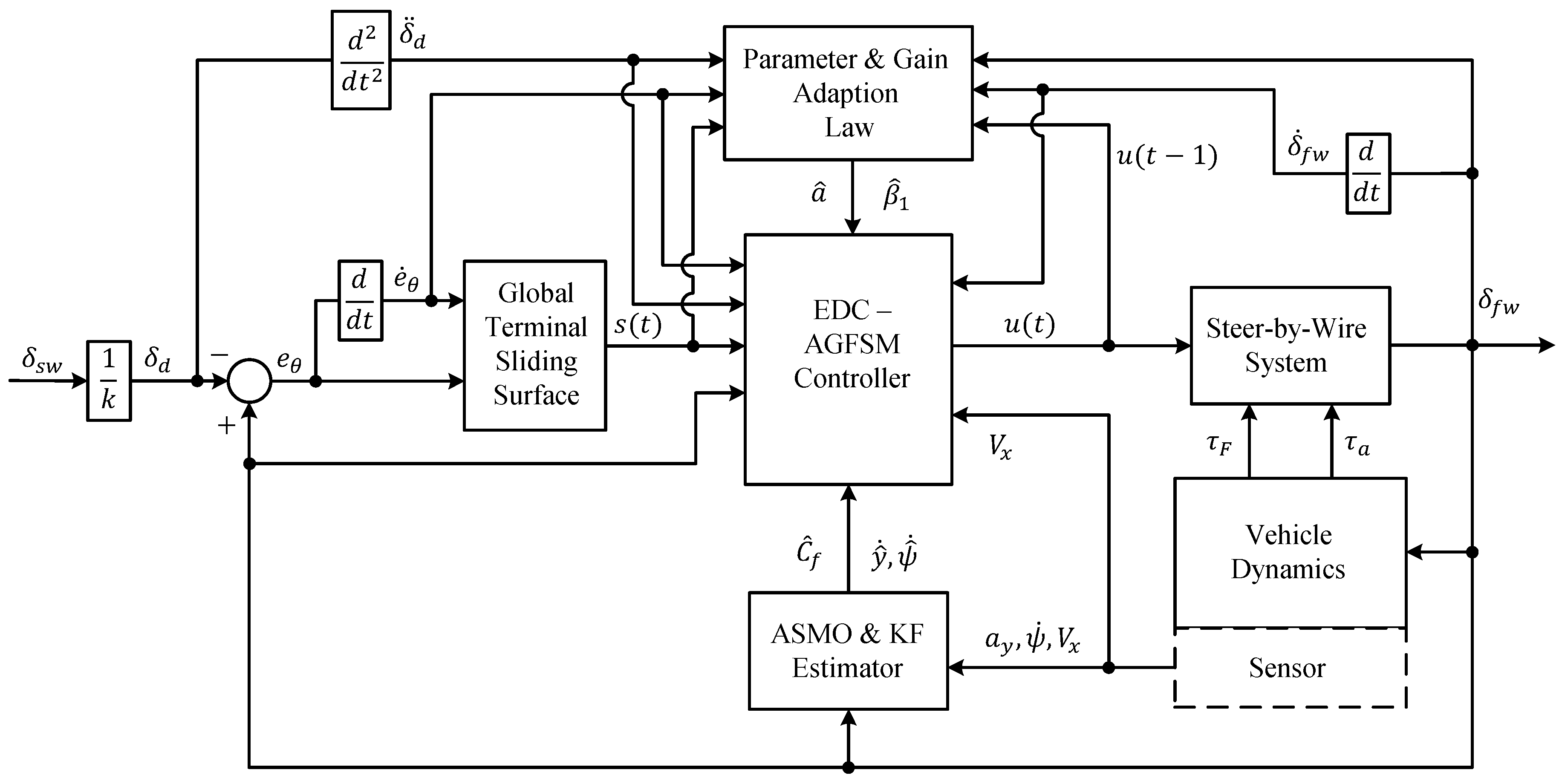
Figure 4 shows the framework of the proposed AGFSMC scheme.
Convergence Proof
The Lyapunov function candidate is defined as:
where
is the parameter estimation error,
is the adaptive gain convergence error, and
is the inverse of gain matrix.
The time derivative of Lyapunov function
in terms of the SbW system (Equation (14)) and the control input (Equation (50)), with the considerations that
,
, are obtained as follows:
It is considered that
and
, such that:
where
and
are the uncertain residual parameters of frictional torque and self-aligning torque, respectively.
Substituting Equations (61), (63) and AGFSMC
(Equation (54)) into (Equation (60)), then the inequality is written as:
With the adaptation laws of
(Equation (57)) and
(Equation (58)), substituting into Equation (63) satisfies:
The convergence proof shows that the proposed AGFSMC is stable and the inequality (Equation (64)) ensures that the global fast terminal sliding surface variable exponentially converges to zero () in the finite time.
Remark 3. The signum function incorporates the chattering and discontinuity in the proposed controller. Therefore, to eliminate the chattering phenomenon the signum function is replaced by the boundary layer saturation function such that Equations (51) and (53) are re-written as: The boundary layer saturation function is defined as:where represents the boundary layer thickness. Due to the boundary layer, the closed-loop error cannot converge to zero. However, a carefully selected value of would lead the error to a user-specified bounded region. Remark 4. In order to avoid overestimation of and , which can lead the control input to saturation, Equations (57) and (58) can be re-written for the permissible bounds of using the discontinuous projection mapping [36] as follows:where and are defined as dead zone bounds [
27]
in terms of tracking error. Therefore, when the tracking error converges to the respective dead zone bound, the adaption mechanism will be switched off and after that and become constant. 6. Simulation Results
In this section, the estimation accuracy of vehicle states and cornering stiffness coefficients, and the control input performance of the proposed AGFSMC scheme for SbW system road vehicles, are validated over the three different maneuvering tests, in compression with adaptive sliding mode control (ASMC) and adaptive fast sliding mode control (ATSMC).
The first test (test 1) is sinusoidal maneuvering with varying tire–road conditions—snowy for the first 30 s and a dry asphalt road for the next 30 s—with the selected coefficient of friction as
,
and the tire cornering stiffness coefficients for the front and rear wheels as
,
,
,
, respectively. The second test (test 2) is known as circular maneuvering, conducted over a dry asphalt road. Moreover, a high speed cornering test (test 3) is also introduced to further evaluate the robustness of the proposed scheme. It is worth noting that the first two tests are carried out at longitudinal speed
and the third test at
with the same sampling rate of
. Furthermore, the vehicle and SbW system parameters are listed in
Table 2.
The parameters for the proposed cooperative ASMO and KF estimator with the termination bounds are selected as: and
In addition, the parameters for the designed AGFSMC scheme with dead zone bounds are chosen as: , , , , , , , , , and the initial conditions are considered as .
To compare the performance of the proposed AGFSMC scheme with the adaptive sliding mode control (ASMC), as designed in [
25], we used the following equations:
where the tracking error
and the sliding surface
with
are defined in Equation (71). The saturation function
is also taken to be the same as Equation (67) with boundary layer thickness
. Moreover, the nominal SbW system parameters
,
,
,
, and the control parameters
,
,
are selected according to the methodology defined in [
25].
For performance comparison with ATSMC, as designed as [
27], the calculations are given as follows:
where
, and
have the same values as those defined in AGFSMC. Moreover, the control parameters and adjustable parameters for adaptive laws are selected according to [
27] as follows:
and
, resptectively.
6.1. Sinusoidal Maneuvering Test (Test 1)
The reference steering wheel angle is generated by:
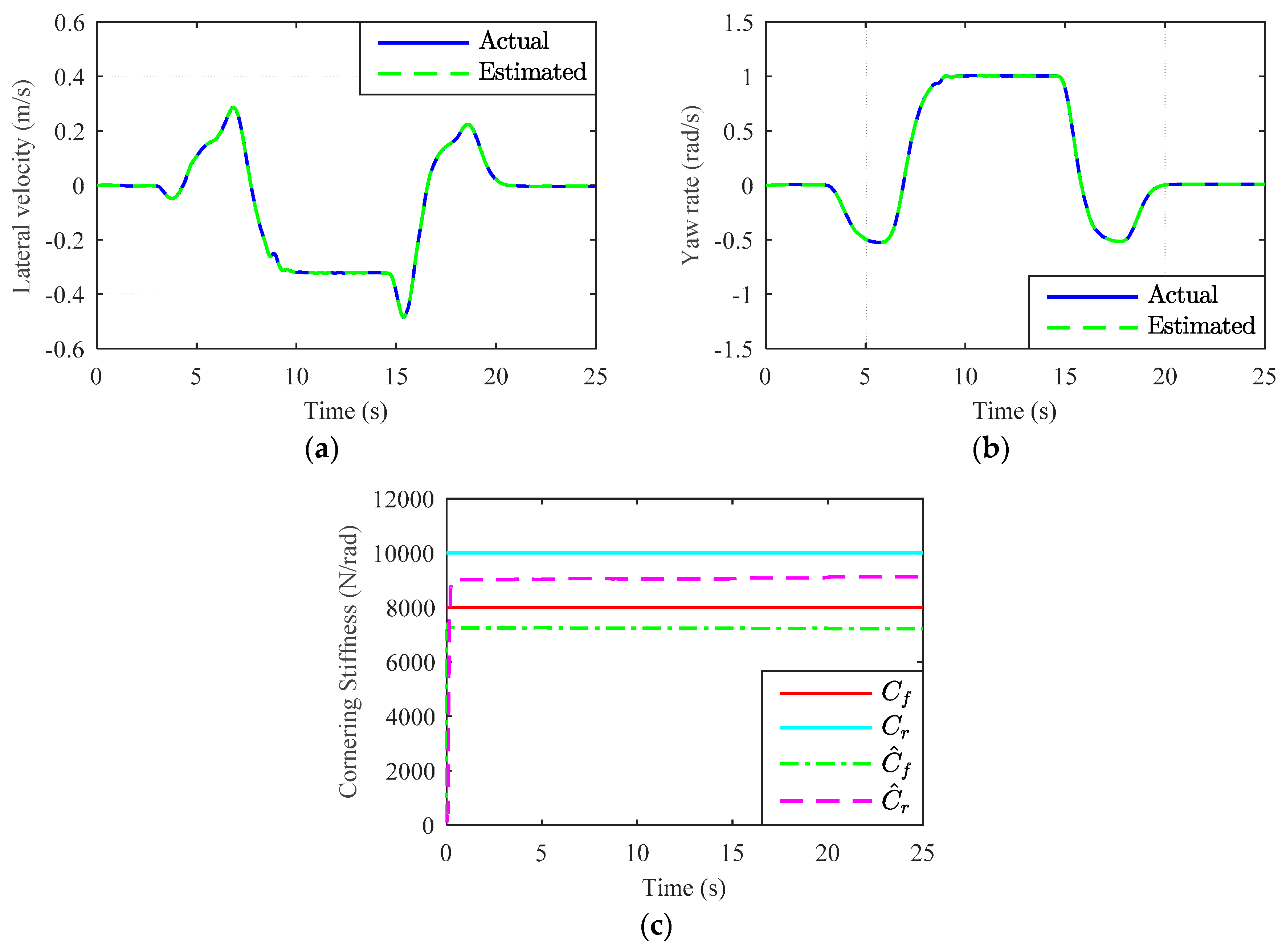
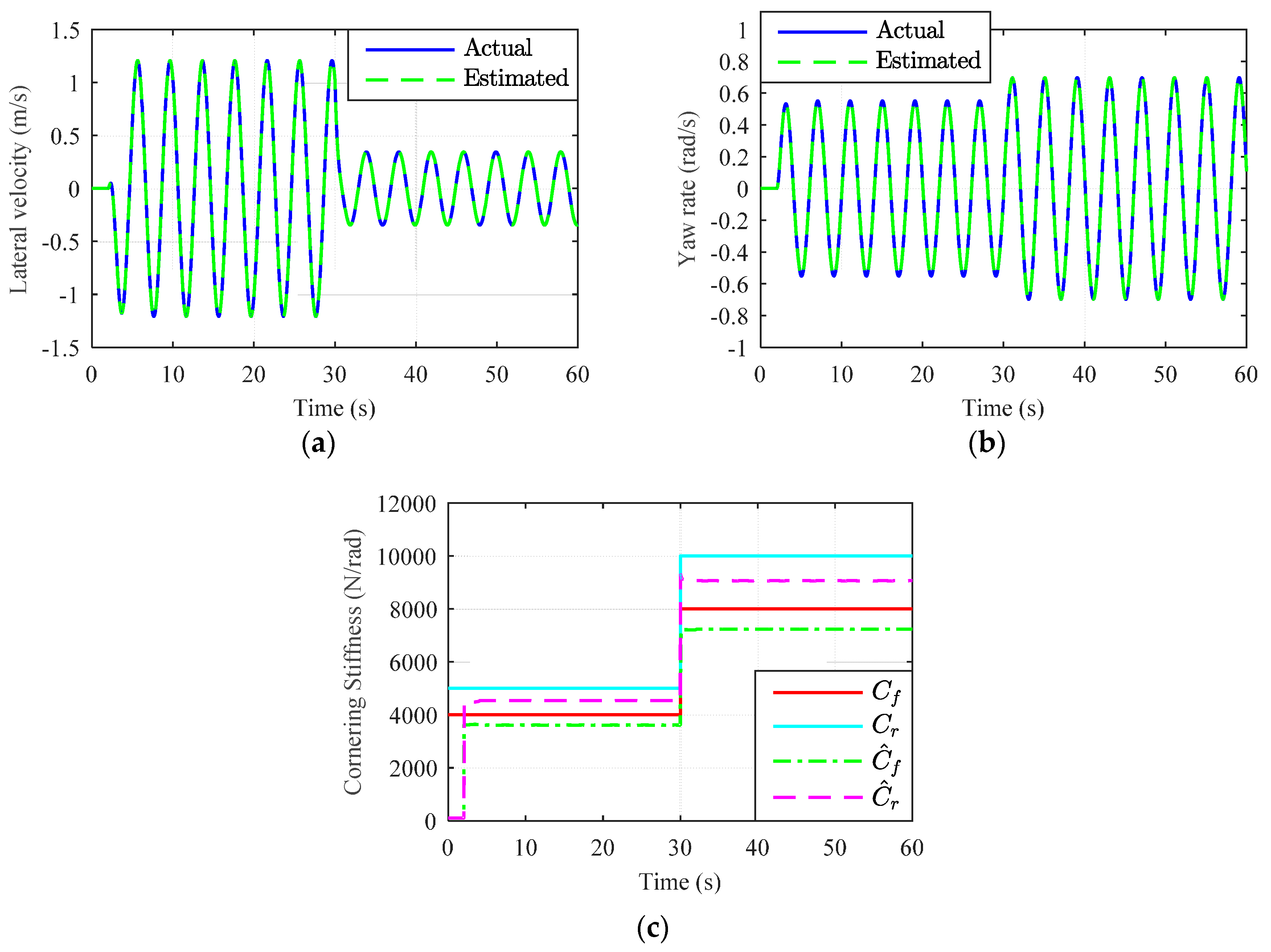
Figure 5 shows the simultaneously estimated lateral velocity, yaw rate, and cornering stiffness coefficients. It is observed that the cooperative ASMO and KF scheme intelligently cope with the tire–road variations and estimate the vehicle states and cornering stiffness coefficients by self-tuning the gains according to the driving environment.
Figure 5c shows that the estimated
have not only converged to the neighborhood of the actual values in both dry and snowy conditions, but also become constant after the condition
reached a specified termination bound.
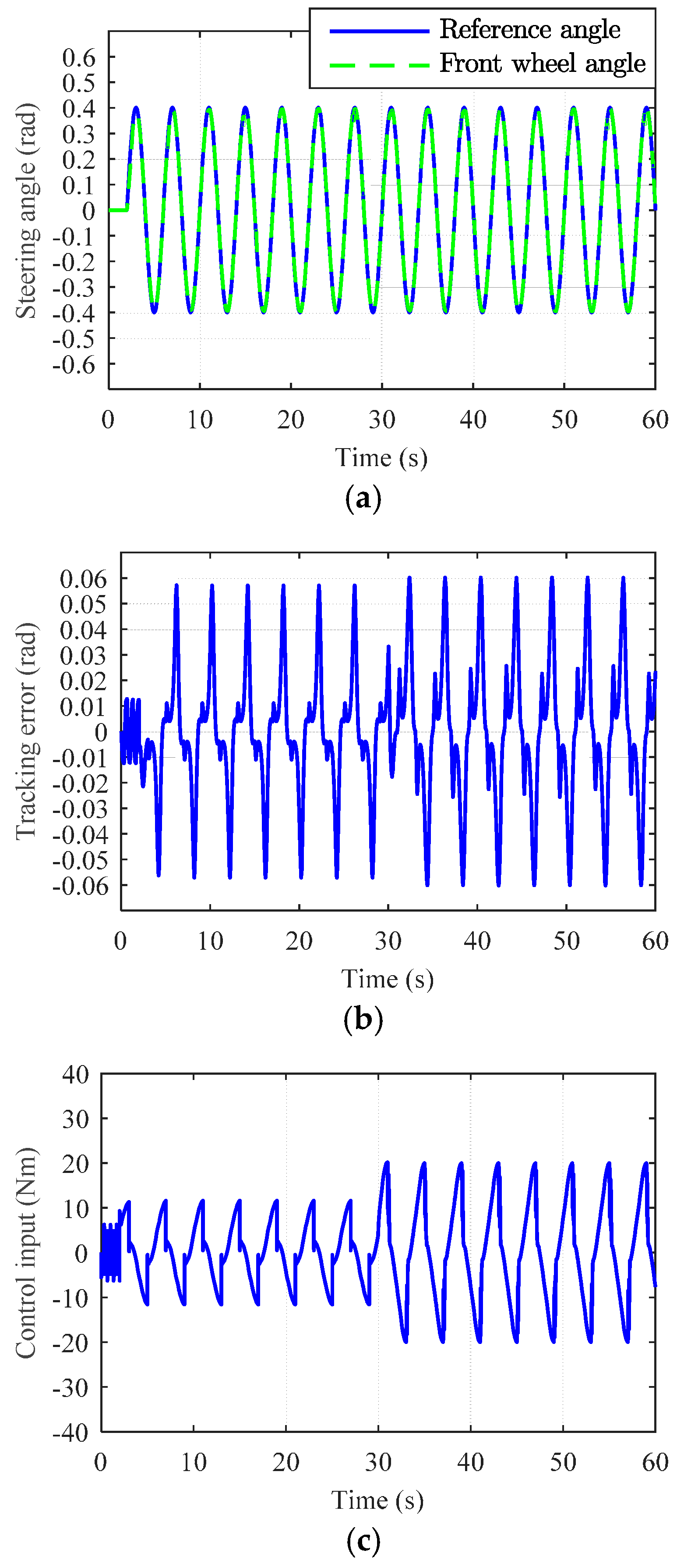
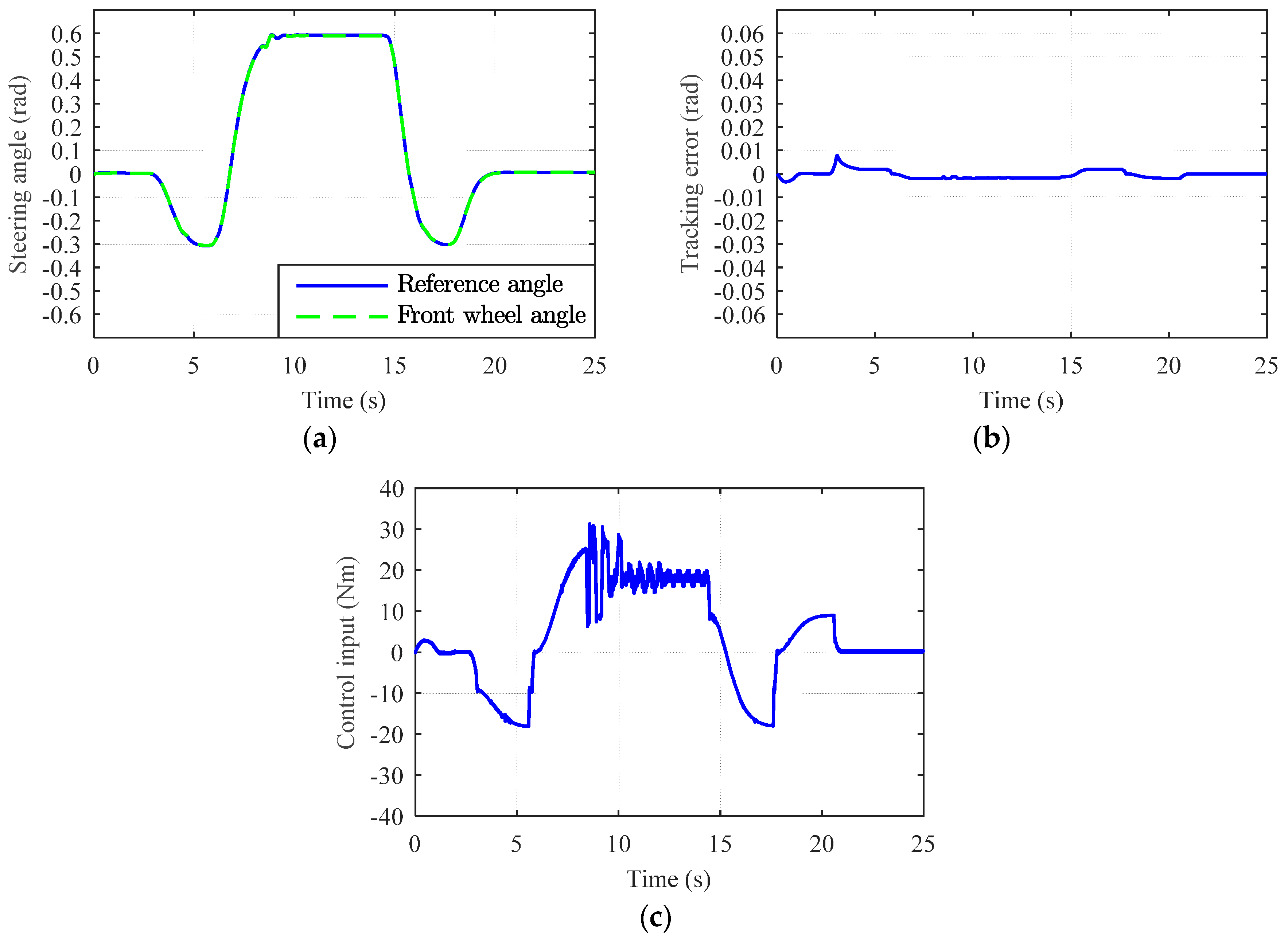
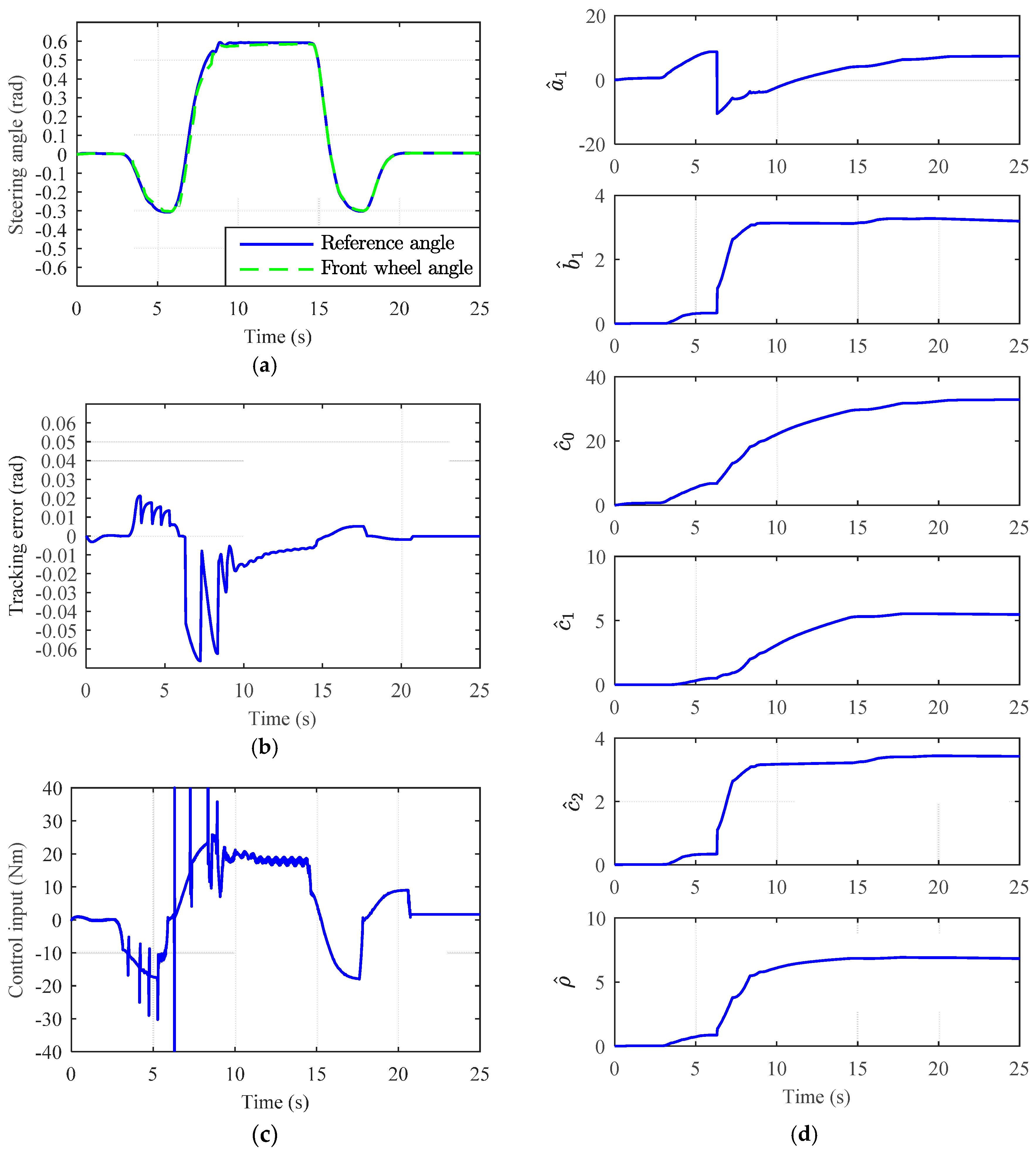
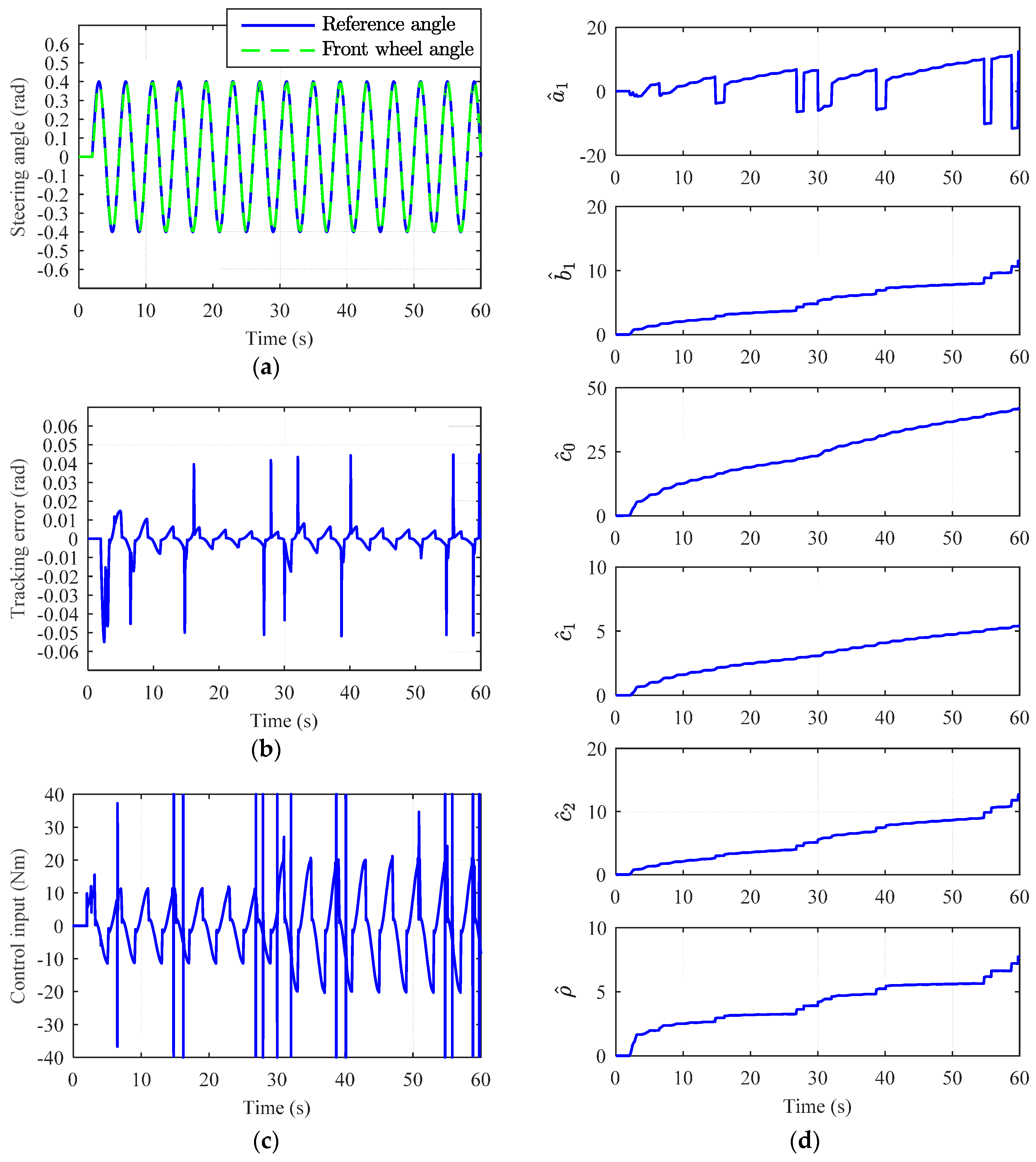
Figure 6 represents the tracking response and the control input performance of the AGFSMC scheme against the varying tire–road disturbance forces. We can see from
Figure 6b that the proposed methodology effectively eliminates the impact of self-aligning torque (Equation (20)) and Coulomb frictional torque (Equation (21)) from the SbW system and ensures that the front wheels are precisely tracking the reference steering angle with a steady state tracking error of
. It is noted that at the beginning of sinusoidal maneuvering, after 3 s, the tracking error reached the peak value of
. This is because we started all the parameter estimations from very low values, such as
,
. Therefore, right after the peak error, all the estimated parameters converged to the sufficient estimation set. As a result, the peak tracking error also converged to the steady-state dead zone region.
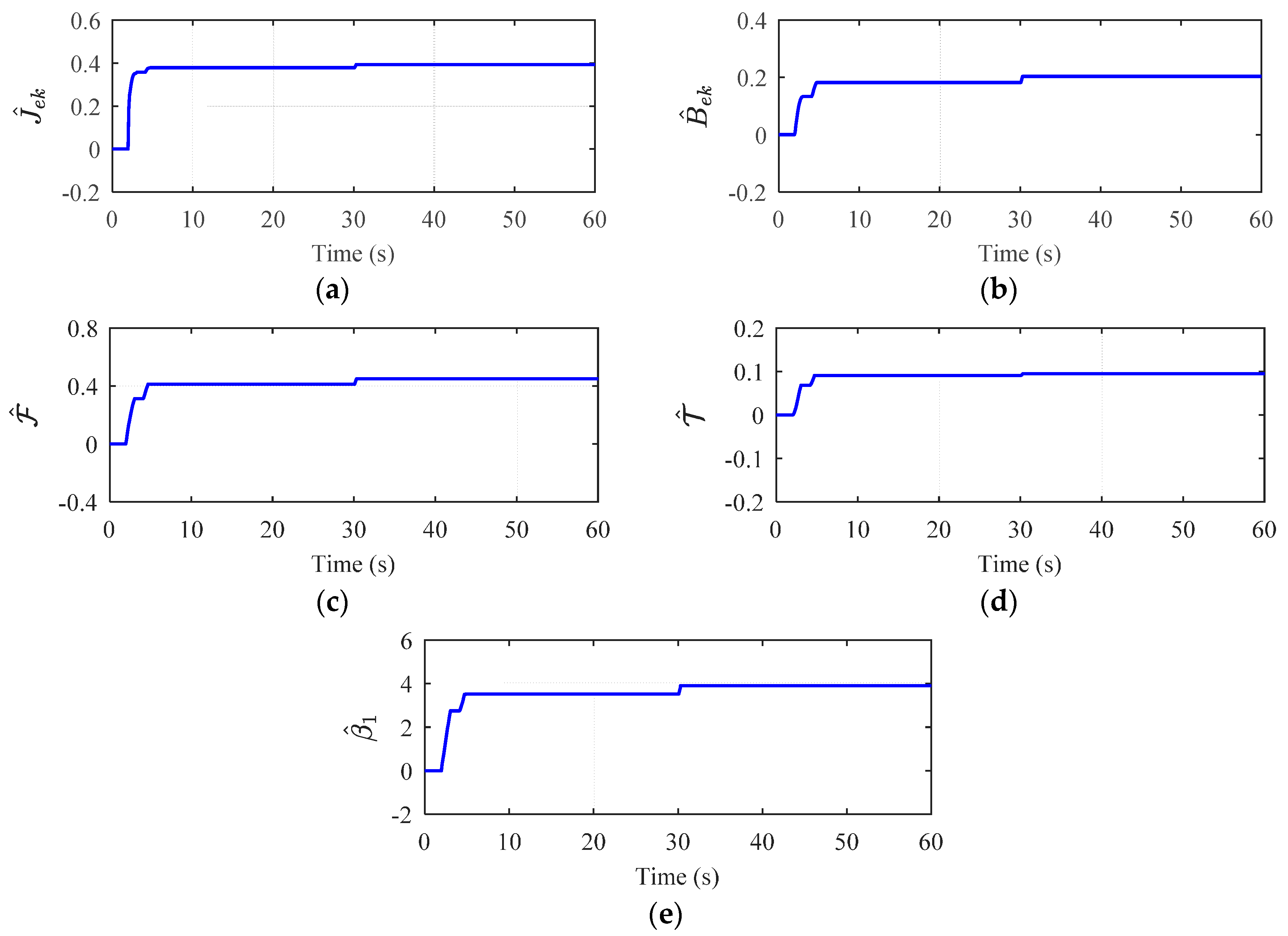
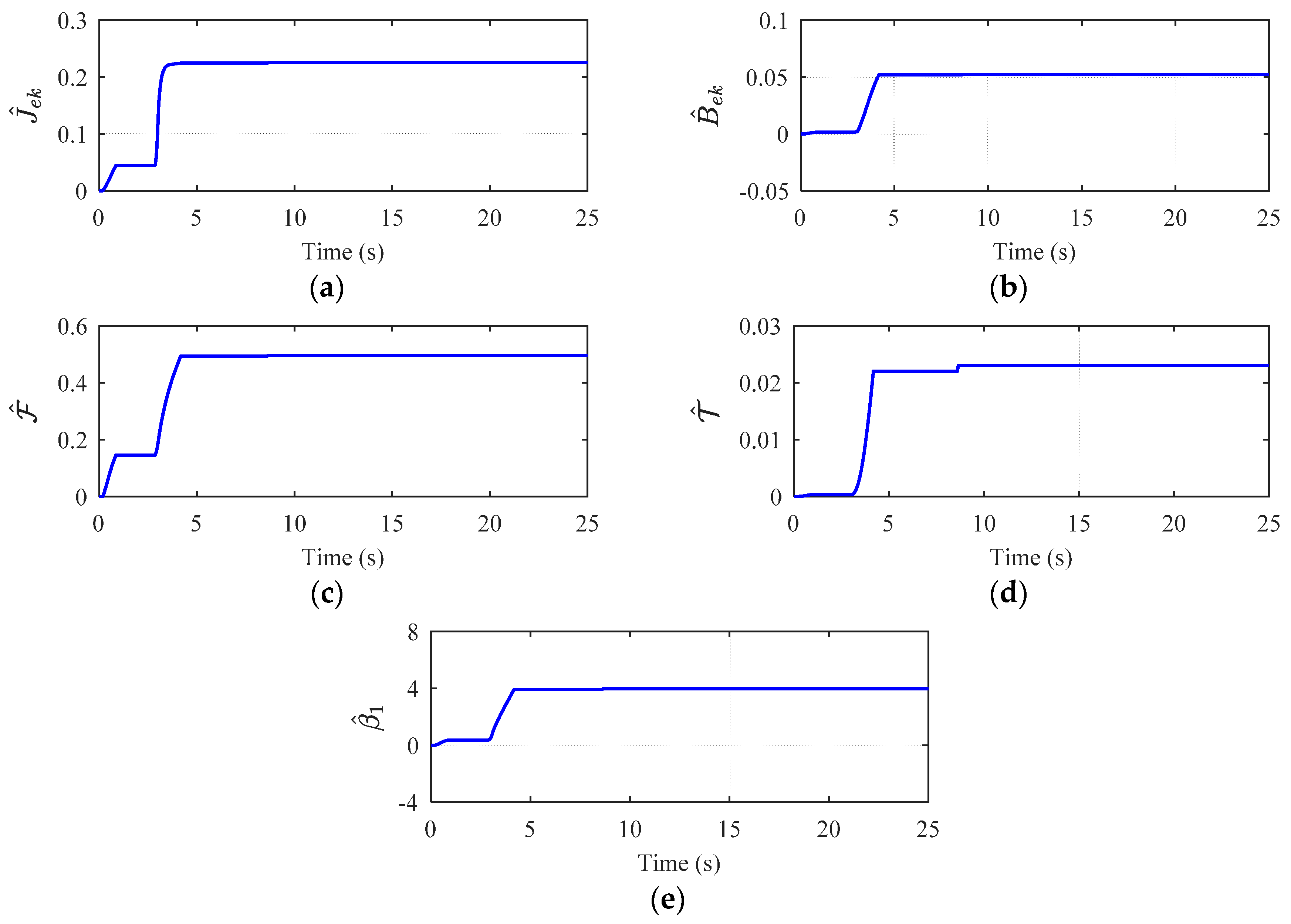
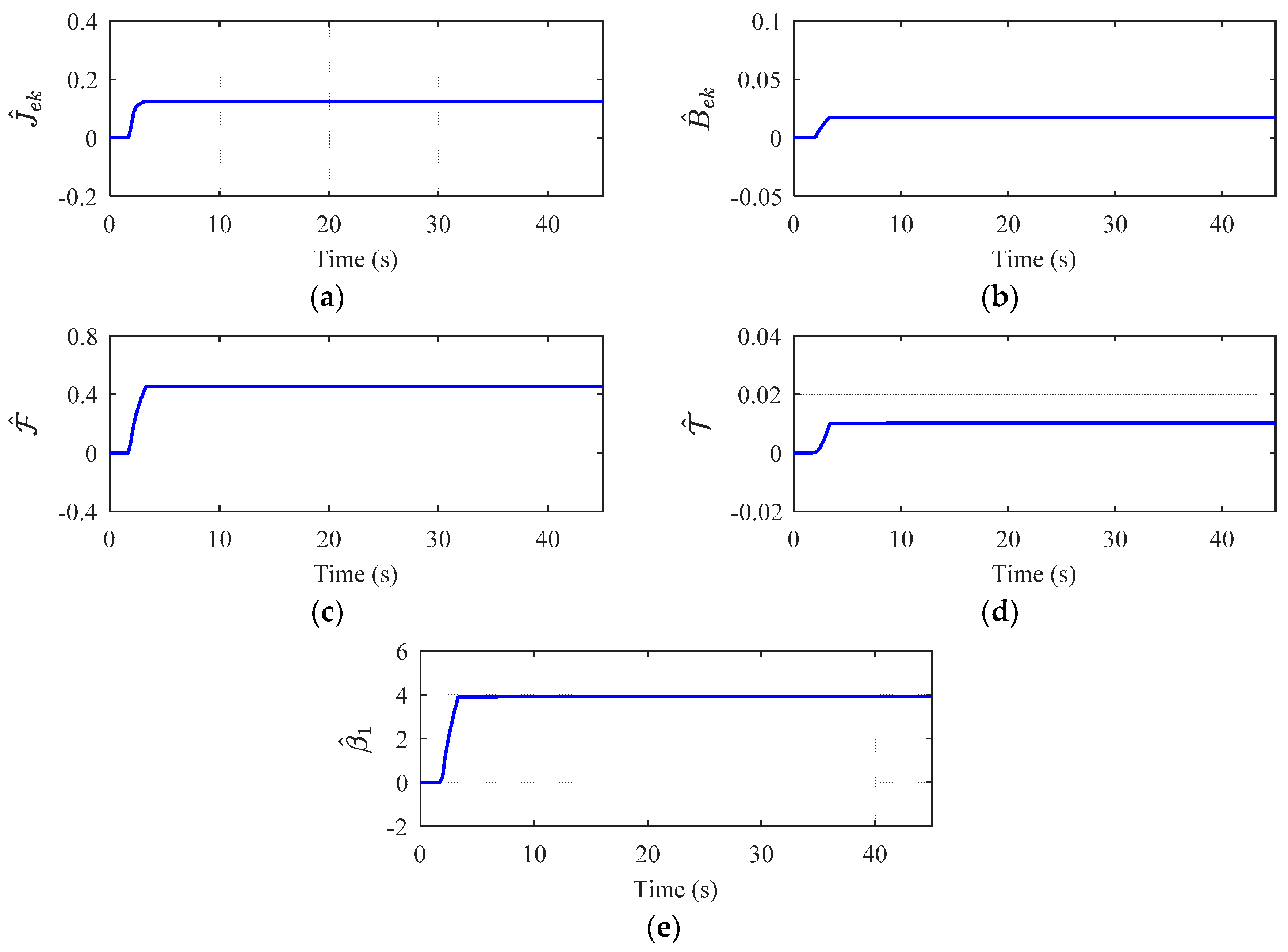
Moreover,
Figure 7 shows the estimated SbW system parameters and the sliding gain adaptation profile. It is observed that the estimated SbW system parameters did not converge to the listed actual constants, but due to the adaptive capability of the proposed control scheme, all parameters as well as the sliding gain are adaptively adjusted in time for both driving conditions, which ensure the closed-loop stability of the SbW system. Hence, the outstanding steering performance of the SbW system vehicle is achieved against the nonlinear tire–road disturbance forces and the uncertain SbW system parameters.
Figure 8 demonstrates that the steering performance of the ASMC scheme is not as good as that of the proposed AGFSMC scheme. This is because the hyperbolic tangent function used in ASMC is unable to replicate the actual self-aligning torque acting on the SbW system. Also, the adaptation law cannot estimate the appropriate equivalent coefficient of self-aligning torque to compensate for the varying tire–road conditions. Consequently, the overall tracking error is much higher, particularly in the dry asphalt road condition: the tracking error peaks to the steady-state value of 0.06 rad, which is almost 30 times higher than in the proposed scheme. Although the ASMC scheme has the information of nominal parameters and utilized the saturation function, it incorporates high-frequency chattering during the first 3 s of the simulation, where the reference angle is set to zero.
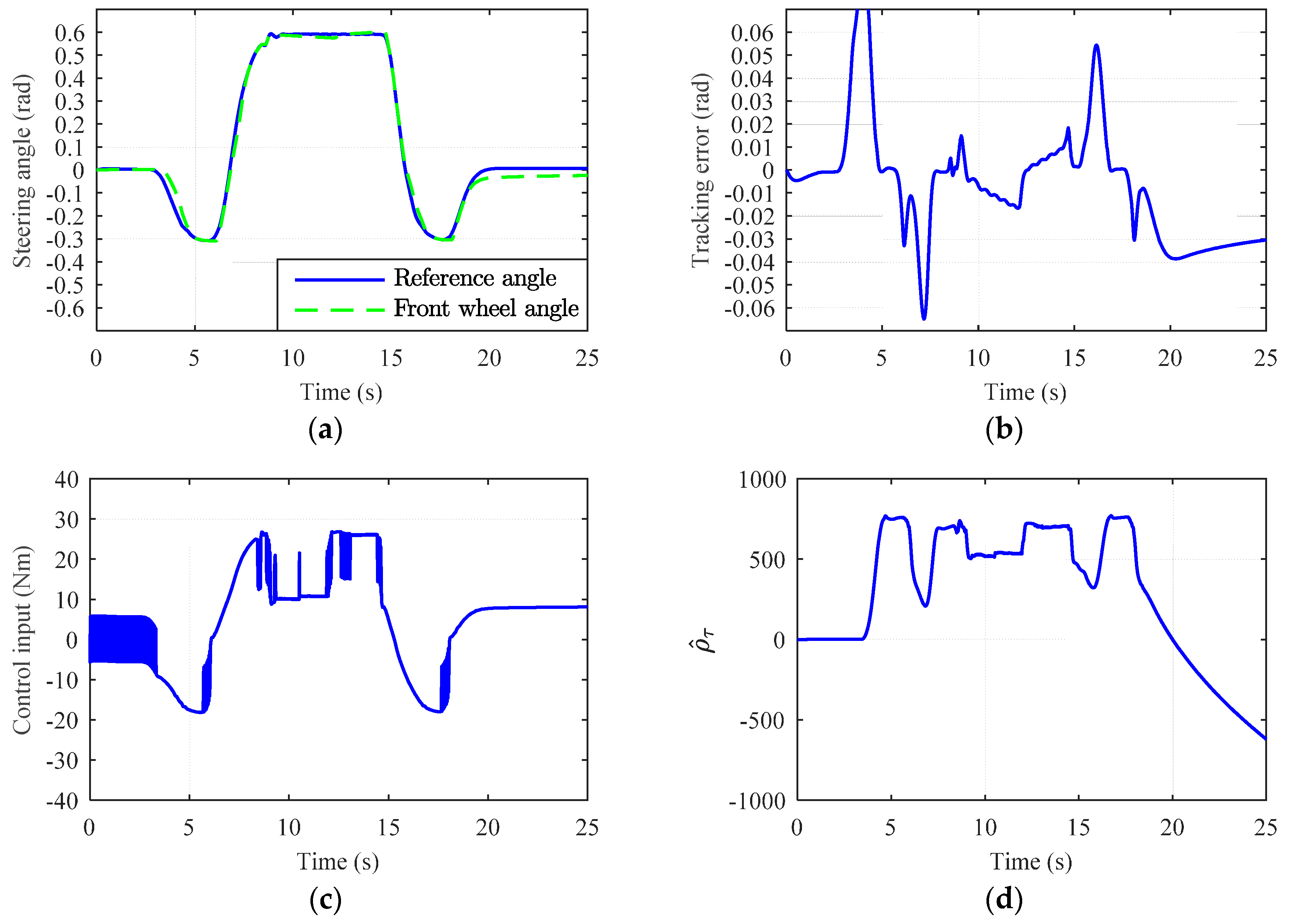
Figure 9 shows that the overall tracking response of ATSMC is better than the ASMC under the varying driving conditions, while both schemes cannot outperform the proposed AGFSMC. It can be seen that the control input overshoots the allowable control limit, which causes irregular spikes in the tracking error. We noticed two reasons for that: (1) The designed adaptation law for estimating the control parameter
does not include a provision to maintain the positive estimation; and (2) the ATSMC does not possess any mechanism to bound or stop the parameter adaptation process for avoiding overestimations, as compared to the one proposed in AGFSMC. Therefore, the tracking error is consistently converging to a smaller region with spikes due to the large and continuous parameter estimation, which may lead the controller to saturation state.
6.2. Circular Maneuvering Test (Test 2)
The circular maneuvering test is carried out over the dry asphalt road for 25 s with these selected tire–road parameters: , and .
Figure 10,
Figure 11 and
Figure 12 portray the promising results of the proposed AGFSMC scheme in all aspects during test 2. We can see the fine estimation of vehicle states and cornering coefficients in
Figure 10. The estimated cornering coefficients takes less than a second to converge to the sufficient estimation set over the dry asphalt, such as,
,
, and becomes constant after
satisfies the selected
bound. Thus,
Figure 11 exhibits the excellent tracking response of the front wheels with an observed peak tracking error of
, which eventually converged to the
bound after the rapid adjustment of all adaptive parameters
and
to certain constants, as shown in
Figure 12.
In contrast to the proposed scheme, the ASMC shows the worst tracking performance throughout test 2. It can be seen from
Figure 13 that the tracking error is unable to obtain any steady state bound and reached a peak value of
, which is almost
times higher than in the proposed AGFSMC scheme. Moreover, the adaptation law also shows inconsistent behavior in the last 7 s of this test, where the estimated coefficient of self-aligning torque rapidly drops to a highly negative value. As a result, neither tracking error nor sliding surface converged to the steady state boundary at a finite time in the Lyapunov’s sense.
On the other hand, the ATSMC performed slightly better than the ASMC in terms of tracking response and also managed to converge the tracking error to the steady state bound during test 2. The peak tracking error observed under the ATSMC scheme is
as shown in
Figure 14, which is marginally less than the ASMC but almost 8.35 times higher than the proposed scheme. Moreover, the abrupt shift in
parameter estimation and the multiple control input overshoots are again observed in this test.
6.3. High Speed Cornering Test (Test 3)
In order to further evaluate the estimation accuracy, tracking response, and control input performance of the proposed AGFSMC scheme, a high-speed cornering test is performed on a dry asphalt road for 45 s.
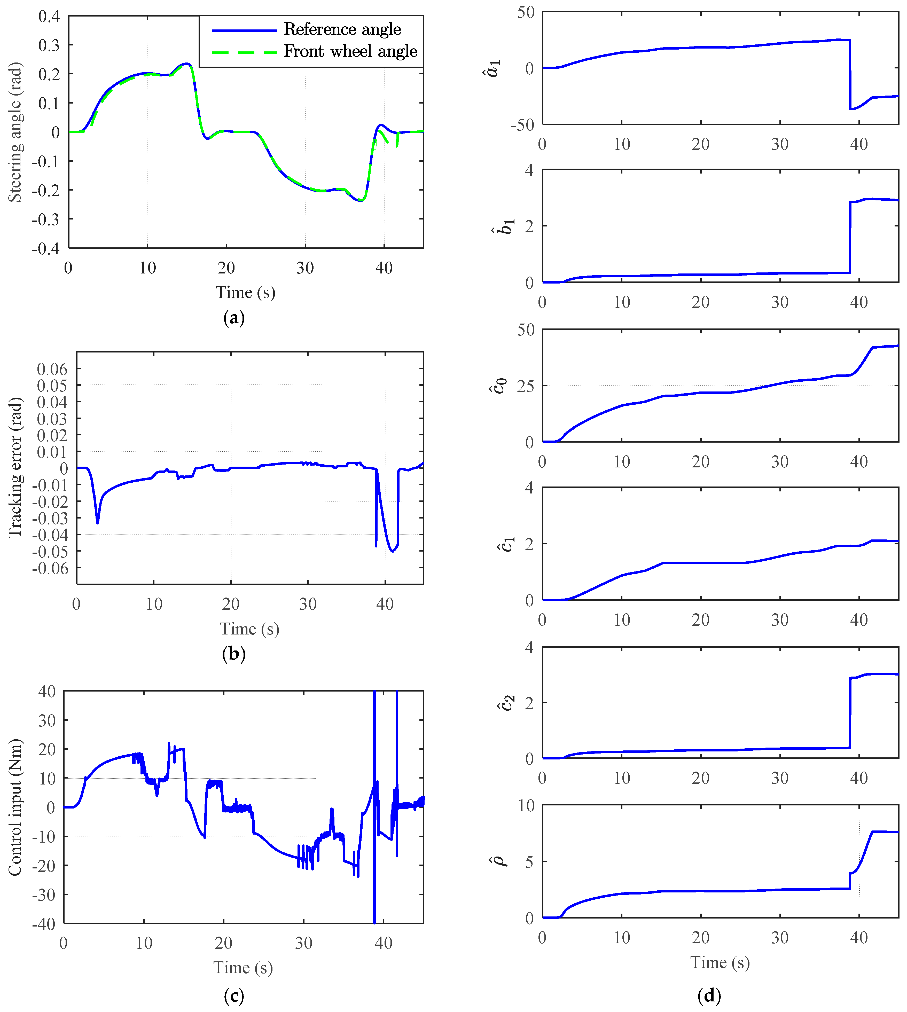
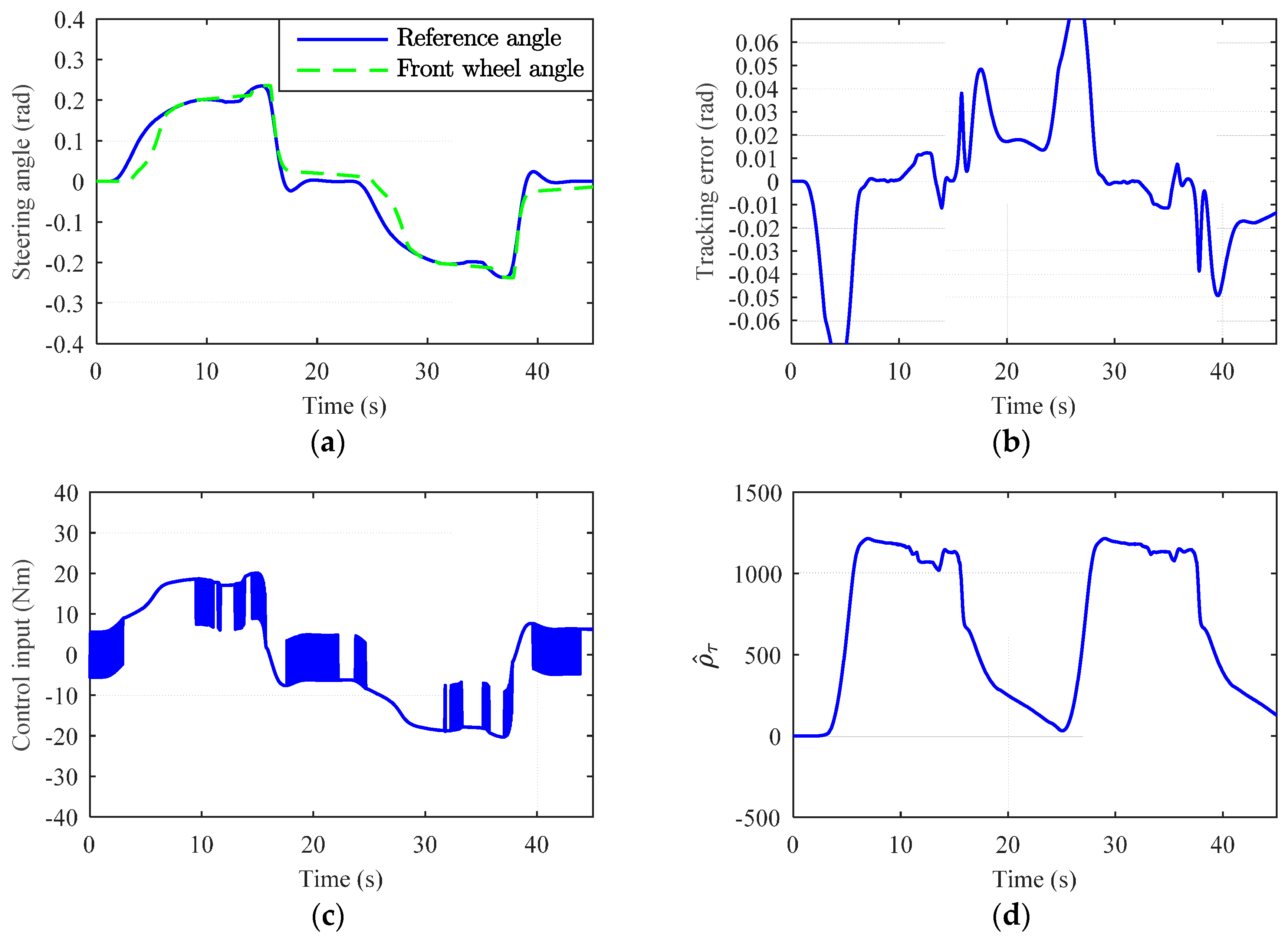
As expected,
Figure 15,
Figure 16 and
Figure 17 clearly indicate the remarkable performance of the proposed scheme against the parametric uncertainties and tire–road disturbance. The cooperative ASMO and KF also maintain the robustness and provide adequate estimated dynamics to stabilize the effect of self-aligning torque and frictional torque at high speed. The peak tracking error observed during test 3 under the AGFSMC scheme is
, which is almost eight times lower than ASMC
, and four times lower than ATSMC
). Compared to other control schemes,
Figure 18 shows that the tracking error under ASMC was again unable to attain any steady state bound and also incorporates high-frequency chattering at constant steering angle inputs. The ATSMC shows a decent performance regarding the tracking error convergence as compared to ASMC. However, the sudden parameter estimation shift with control overshoot still exists in this test, as shown in
Figure 19.


