Data-Foraging-Oriented Reconnaissance Based on Bio-Inspired Indirect Communication for Aerial Vehicles

Abstract

In recent years, aerial vehicles have allowed exploring scenarios with harsh conditions. These can conduct reconnaissance tasks in areas that change periodically and have a high spatial and temporal resolution. The objective of a reconnaissance task is to survey an area and retrieve strategic information. The aerial vehicles, however, have inherent constraints in terms of energy and transmission range due to their mobility. Despite these constraints, the Data Foraging problem requires the aerial vehicles to exchange information about profitable data sources. In Data Foraging, establishing a single path is not viable because of dynamic conditions of the environment. Thus, reconnaissance must be focused on periodically searching profitable environmental data sources, as some animals perform foraging. In this work, a data-foraging-oriented reconnaissance algorithm based on bio-inspired indirect communication for aerial vehicles is presented. The approach establishes several paths that overlap to identify valuable data sources. Inspired by the stigmergy principle, the aerial vehicles indirectly communicate through artificial pheromones. The aerial vehicles traverse the environment using a heuristic algorithm that uses the artificial pheromones as feedback. The solution is formally defined and mathematically evaluated. In addition, we show the viability of the algorithm by simulations which have been tested through various statistical hypothesis.

1. Introduction

In recent years, the use of Unmanned Aerial Vehicles (UAVs) has become important in numerous tasks, such as security surveillance, transportation [1], rescue and environmental monitoring. An outstanding capacity of these vehicles is that they can allow not only monitor environments with harsh conditions where humans cannot have access, but they can also monitor scenarios that change periodically, with a high spatial and temporal resolution [2].

For example, in flood monitoring it is necessary to identify the increase in water levels of certain regions in the environment. The water level can move in an uncontrolled way and change with a high frequency. Therefore, to identify these changes it is necessary to perform reconnaissance (Reconnaissance refers to the task of traveling with the purpose of discovering new territories, unknown spaces, roads and routes.) tasks over an area. This implies frequently collecting and selecting the most relevant data about the current status of the environment. Once the reconnaissance task has been done, oversampling some regions is necessary to determine which regions are relevant despite changes in the environmental conditions.

A feasible solution is to employ UAVs to perform the reconnaissance task. In this sense, some UAVs can sample the area through various flights, exchanging partial views to determine the regions with relevant environmental data. However, due to their mobility, UAVs have inherent constraints in terms of energy and transmission range. Thereby, it is necessary not only to perform the communication among these vehicles even with a lack of direct coupling among senders and receivers, but also to tackle the problem of monitoring a changing environment.

In nature, some animals face similar problems when foraging for food, and the main objective is to retrieve the most profitable food resources by considering various restrictions, including energy. In order to communicate the findings obtained through reconnaissance to other animals, several species use indirect communication such as segregation of pheromones. Data Foraging is related to the selection of profitable data sources in a dynamic environment with mobile sensors.

Many approaches related to reconnaissance with mobile sensors have been proposed, especially in robotics, where the main objective is to find an optimal path to maximize the knowledge over a particular area [3,4,5,6,7,8].

Finding a single optimal reconnaissance path is not suitable for data foraging, particularly when an operational environment with highly changing attributes is considered, and where the objectives may change dynamically.

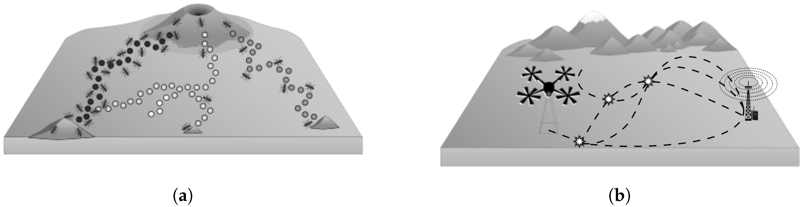
In this sense, Data Foraging-Oriented Reconnaissance (DFORE) requires establishing multiple dynamic paths to ensure that a profitable data source can be identified. Figure 1a depicts how a group of ants performs the exploration and the exploitation of their environment. In some species, food collection is achieved by thousands of workers travelling along well-defined foraging trails. These trails emerge from a succession of pheromone deposits that can result in a complex network of interconnected routes [9]. To perform DFORE, a UAV searches for points of interest in an unknown environment, as depicted in Figure 1b. Through various trips, the UAV can identify a region which has something of interest to the application. Both systems are dynamic; therefore, several paths must be explored in order to exploit useful resources.

In this work, we propose a Data Foraging-Oriented Reconnaissance algorithm for a single aerial vehicle. Inspired by the stigmergy principle, aerial vehicles communicate indirectly through an artificial pheromone to create several paths and to explore the operational environment with limited movement capabilities; thus, the focus of the research is how these devices through indirect communication can do a reconnaissance task. A hexagonal grid to represent the operational environment is used. Hexagonal models allow for a better movement representation in 2D due to the uniform distance in any direction. We assume the aerial vehicle has limited movement capabilities, and for this reason, the aerial vehicle needs to be recharged as many times as needed at a base station. The required movement capacity of the aerial vehicle per trip to explore an operational environment is identified based on the size of the hexagonal grid. The algorithm accomplishes the temporal constraints that are defined for DFORE. It is proved in a formal way that the algorithm satisfies such constraints. A computational cost analysis and a simulation are presented to show the viability of our solution. We compare our proposed algorithm to MULES [10], adapted to the foraging reconnaissance task, which is a random walk with uniform distribution algorithm to collect data from the environment. MULES has similarities with our proposed mechanism, they both use indirect communication through an intermediary in our case artificial pheromones and in MULES the use of a mobile data relay. We measured the number of trips by each algorithm in different conditions. The comparison with MULES is justified since this proposal is the baseline algorithm for indirect communication among mobile sensors. Also, this algorithm is extensively used in recent works to solve problems like patrolling, source location privacy, data collection, etc. [11,12,13].

The organization of this document is as follows: A survey of recent literature is presented in Section 2. In Section 3, the preliminaries are explained along with the system model. Our proposed solution is presented in Section 4. The analysis of the proposed algorithm is shown in Section 5. In Section 6, the proof to validate our proposed algorithm is discussed. A series of experiments are shown in Section 7. The discussion of our algorithm is presented in Section 8. Conclusions are presented in Section 9. As a quick guide to follow this work, the notation is presented in

Table 1. Notation table.

U	≜	Set of Mobile Data Foragers, where each $u\in U=\{u_1,u_2,\cdots ,u_q\}$
R	≜	The operational environment represented by a set of regions r
H	≜	The Hextille that represents the operational environment
$G_h$	≜	The Data Foraging graph to model Hextille H with radius $h_{ex}$
$n_h$	≜	Number of cells of $G_h$
$p_h$	≜	Depth of $G_h$
${ϵ}_h$	≜	Required steps to traverse $G_h$
$e_u$	≜	Endurance of mobile sensor u
$F_c$	≜	Set of food pheromones
$F_t$	≜	Set of travel pheromones
F	≜	Set of pheromones. The union of $F_c\cup F_t$
$F_r$	≜	The set of pheromones present at region r
$\eta$	≜	The farthest region from the base within the main line
$\zeta$	≜	The region r where the base station is located
$T_{expMax}$	≜	Maximum reconnaissance time
$Tstart$	≜	Reconnaissance’s start time
$Tstam{p}_t\left(r\right)$	≜	The time when the region r is stamped

.

2. Related Work

There are several remarkable works related to our proposal from different perspectives. In this section, the related work for constrained exploration is presented, where a mobile agent must interrupt, return to the base station and refuel before continuing exploration. Next, the works that address the reconnaissance problem are discussed, which is a special type of exploration where the objective is to gain strategic information from uncertain environments with an optimal path. Finally, the differences between reconnaissance and Data-Foraging Oriented Reconnaissance are presented.

2.1. Constrained Exploration

Exploration of an unknown environment has been studied in numerous occasions [14]. In most proposals, the unknown environment is modeled as a graph. For such approaches, the task is to explore a given graph while optimizing the exploration routes. In general, exploration algorithms can be classified into two main types: offline and on-line. Offline exploration occurs when the graph information is known in advance. In contrast, during an on-line exploration, the information about the graph can only be learned in the execution of the exploration algorithm. Based on the concept of on-line exploration, the most used algorithms are the Depth First Search (DFS) and the Breadth First Search (BFS) [15]. A variation of on-line exploration was introduced by Betke et al. [16]. In this variation, called piecemeal search model (PSM), two constraints were added to the problem of graph exploration:

• Continuity: An agent must traverse the graph by passing through incident nodes. There is no teleportation of the agent to any node.
• Interruptibility: The agent must return to the start node s after traversing $\vartheta$ steps to recharge energy, where $\vartheta$ is a constant . In this sense, for PSM, the agent’s energy (required to travel $\vartheta$ steps), is set to $2(1+\alpha )r$; where r is the distance to the farthest node from the starting node s and $\alpha >0$ is a constant. The agent’s energy is proportional to $\alpha$.

With these constraints, BFS and DFS are not able to solve the piecemeal search problem [17]. Thus, several algorithms have been proposed to tackle such a problem. Betke et al. [16] present two algorithms: Wavefront and Ray. The Wavefront algorithm is based on BFS. It expands knowledge in waves from a starting node, just like a pebble expands a wave when thrown in a pond. The graph is decomposed into four regions, and each region is explored through ripples. The authors also present an algorithm based on DFS, which is called Ray and is similar to Wavefront, but it considers the shortest path from the starting node and any point in the ray. The main objective of these algorithms is to reduce the uncertainty of new routes to traverse an area. To the best of our knowledge, there are only three more works that deal with the restrictions proposed by Betke et al. [16]: Argamon et al. [18], Duncan et al. [17], P. B. Sujit and Debasish Ghose [19]. Moreover, in opportunistic routing, Shah et al. [10] presented another work that can be extended to satisfy the PSM constraints.

Argamon et al. [18] present an on-line exploration while performing algorithm for a repeated task(s). A repeated task must be done continuously, more than once. An agent needs to go from two points at least r times. The goal of the agent is to minimize the overall cost of performing the task(s). The agent also searches for new paths in the graph that are not explored. Movement is done through the expected utility of each path taken. The path between the two known points, improves over time. This movement is not restricted by energy constraints, and it is assumed that the agent has enough energy to get to the two points.

In Duncan et al. [17], the authors present an optimal constrained graph exploration algorithm called Bounded Deep First Exploration (bDFX), which uses a rope of size $(1+\alpha )r$ for some constant $\alpha >0$ and a known radius r. To be able to access every node in the graph, bDFX prunes the nodes beyond the rope and maintains a list of disjoint subtrees of the original graph whose union contains all the nodes not visited. After applying a deep first search algorithm to each subtree, an agent can visit all the nodes of that particular subtree.

P. B. Sujit and Debasish Ghose [19] introduce game theory, where two UAVs explore an area in order to minimize the uncertainty of the sampling area. They proposed computing a non-cooperative Nash equilibrium to coordinate the two UAVS. However, it is very expensive to compute it. Furthermore, they have a q-ahead look-up policy, which makes calculating the Nash equilibrium even more costly.

In opportunistic routing, mobile sensors have uncontrolled mobility and move in a random fashion, similar to a random walk. Despite not using the constraints of the PSM, Shah et al. [10] proposed a three-tier architecture with a mobile sensor named Data Mobile Ubiquitous Local Area Network Extensions (MULEs) to collect data from sensors and transfer them to the sink. Thus, the MULEs are a mechanical carrier of information and achieve indirect communication between sensors. In order to include the constraints of the PSM, it is necessary to limit the movement of the MULEs and make them return to a base station after some steps. Using the approach of indirect communication, the network life is extended as indirect communication removes the burden of control information from the sensor, although latency is increased because the sensors have to wait for a MULE to approach before they can transfer data. As a result, high latency is the main disadvantage of such approaches.

2.2. Reconnaissance Problem

There have been many works that tackle the reconnaissance problem with aerial vehicles. Most of them are focused on the path taken by these aerial vehicles; thus, the interest is to find the optimal path under a series of constraints. Strategic information is represented as targets. The targets can remain fixed or change with respect of time, i.e., the operational environment is dynamic and uncertain. Therefore, the task of reconnaissance is divided into two approaches: Static and Dynamic.

Static path optimization relies on knowledge about the operational environment. Traditional approaches such as Particle Swarm Optimization [20], Genetic Algorithms [21] and Ant Colony [22] are used to obtain an optimal path for the aerial vehicles. Several other constraints to find an optimal path have been studied. Time is one of them; thus, the problem of task assignment has been researched in [23,24]. The minimum number of turns required to cover an area is explored in [25]. Formation for several aereal vehicles is also analysed in [26]. There are also others interesting optimization approaches based on techniques like Taguchi-methods, differential evolution, hybrid Taguchi-cuckoo search algorithm [27,28,29] that have given nice result optimizing objectives in multiples scenarios such as two degrees of freedom compliant mechanism, micro-displacement sensors, and positioning platforms.

The main disadvantage of these approaches regarding an unknown environment is the assumption of information known a priori. Another issue is that the optimal path obtained by these approaches must remain constant; however, there are dynamic environments where new conditions must be taken into account in order to get a useful path, e.g. the aerial vehicles must avoid moving obstacles. Dynamic reconnaissance for unknown environments has been studied in the following works. The aerial vehicles must respond to the dynamic changes in the environment. The use of probability distributions with a priori information has been addressed in [30,31], where the main idea is to adapt the path taken by the aerial vehicles based on the probability of new threats or emerging targets. To avoid obstacles, a hybrid approach was proposed in [32].

2.3. Differences between Reconnaissance and Data-Foraging Oriented Reconnaissance

There are differences between common reconnaissance and Data Foraging-Oriented Reconnaissance (DFORE). In common reconnaissance, every node must be visited with equal priority, and a single trip is sufficient to gather data from the nodes. However, for DFORE, the priority of every node can change based on the retrieved information of the node; thus, the interest is to overlap several trips. Therefore, in the common reconnaissance problem, the movement capability to traverse the whole graph is greater than the number of nodes: $ϵ\ge \alpha n$ where $ϵ$ is the movement capability a mobile agent has, $\alpha >1$ is a constant and n is the number of nodes. Then, the objective is to minimize $ϵ$ with an optimal route because every node has the same priority. On the other hand, DFORE considers multiple trips to explore the whole graph due to the movement constraints of the mobile elements. Thus, the objective is to obtain valuable data sources based on the overlapping paths generated by several trips in unknown environments. Most of the cited works do not meet the constraints imposed by DFORE, with the exception of MULES [10] modified to have movement constraints. The objective of our work is to explore a delimited area with endurance constraints for a dynamic environment by using a single aerial vehicle to obtain valuable data sources, which meet the constraints of the DFORE problem.

3. Preliminaries

In this section, the system model, as well as the formal definition of DFORE with its restrictions, are discussed.

3.1. Problem Definition

The problem of DFORE is related to the reconnaissance task in uncertain environments, where valuable regions can change with respect to time due to their dynamic nature. More precisely, each profitable region has a lifetime associated to it. Each of these regions has different values according to the application. Considering the conditions of the operational environment, it is necessary to oversample it through various trips and to selectively choose the more profitable regions, taking into account the temporal constraints of the regions. Therefore, the reconnaissance step must ensure that the entire sampling area is examined before a maximum time $t_1$.

3.2. Modeling the Operational Environment

Exploring the operational environment is done through a single aerial vehicle. The aerial vehicle lifts off the base station $\zeta$, explores the operational environment, and returns to the base station to refuel. These three activities, together, determine a trip. Due to the flight endurance, which refers to the amount of time a mobile element spends in flight without landing, it might be impossible to visit all the regions of the operational environment in a single trip. In this work we assume that the mobile element must return to a base station to recharge fuel; that is, the flight endurance of the mobile element is not enough to explore the whole environment. For these reasons, the aerial vehicle needs to perform several trips in order to explore the operational environment.

3.3. System Model

Next, the system model is defined in order to describe and represent our system.

• Mobile Data Foragers. The explorer entities in the system are modeled as MDF. Each MDF belongs to the set $\mathit{U}=\{u_1,u_2,\cdots ,u_q\}$. An MDF $u\in U$ represents aerial vehicles flying over the operational environment. Each $u\in U$ has a finite amount of steps it can make, limited storage and computational resources. Every time the MDF moves to an adjacent region, the number of steps of the MDF is reduced by one.
• Pheromones. Since there is no single reconnaissance route, each MDF $u\in U$ is guided by a trail of pheromones. In this work, a pheromone is defined as an abstract data type as follows. A pheromone $f\in \mathit{F}$ is represented as a tuple $f=\{r,\mathit{counter}\}$, where r is the identifier of the region where the pheromone was placed, and counter is the number of pheromones placed in such region. There are two types of pheromones: food and travel pheromones. Food pheromones indicate that in a specific region there is something of interest to the application; food pheromones are denoted by the set $F_c$. On the other hand, travel pheromones indicate that the region has been visited; they are denoted by the set $F_t$. The set F of pheromones is the union of food and travel pheromones, that is $F=F_c\cup F_t$. Each pheromone belongs to the set $\mathit{F}=\{f_1,f_2,\cdots ,f_k\}$. Each pheromone f has a lifetime associated to the maximum time a pheromone can be in a region.
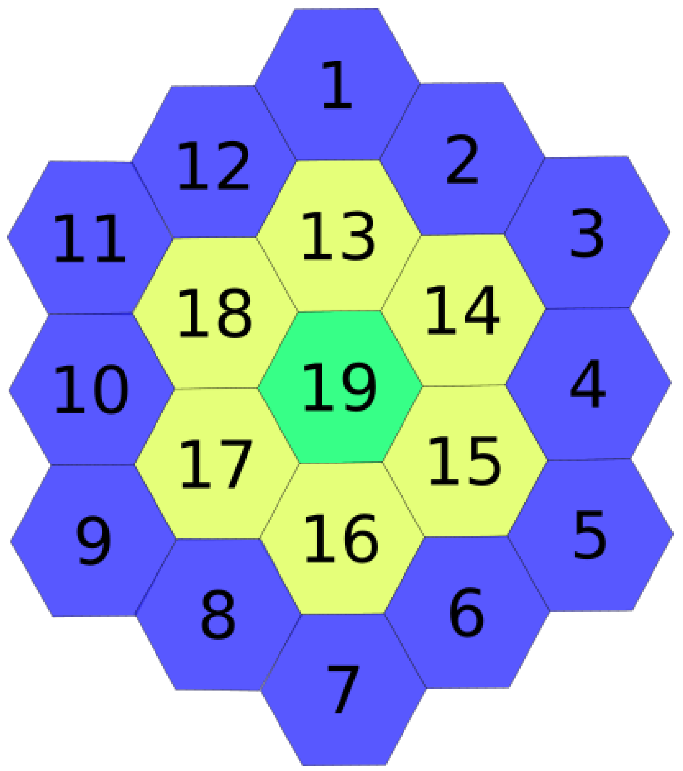
• Operational environment. We represent the operational environment as a Hextille H of radius $h_{ex}$ in the form of a set $R=\{r_1,r_2,\cdots ,r_i\}$, where each $r\in R$ is a sampling region. The radius $h_{ex}$ of the Hextille H is defined as the linear distance from the center of the Hextille to the farthest hexagon of the Hextille in any of the six directions. Figure 2 shows an example of the environment as a tilled hexagonal grid. It should be noted that the hexagonal grid is not restricted just to the specific radius shown in Figure 2 and can vary in radius. A two-dimensional space is considered along with the knowledge of the environment in the form of a map, but without the characteristic and conditions of the environment; that is, there is no information about where valuable data sources are located. Exploring the environment is done through one MDF. The MDF starts at the base station, explores the environment, and returns to the base station to refuel; this is called a trip. The sampling area is a subset $S\subseteq R$, where each region $r\in S$ is a hexagon with a diameter equal to the sensing range of an MDF $u\in \mathit{U}$. Only one $u\in U$ can be in the environment at any given time. It should be noted that each region $r\in S$ has dynamic changing conditions, which means that regions that are valuable do not necessarily remain valuable indefinitely. Each $r\in R$ has a number of pheromones f $\subseteq F_r$, where $F_r$ is the set of pheromones present at region r.
• Base station. The base station $\zeta$ is a processing unit, associated to the physical place where each MDF lifts to explore the environment and drops the retrieved data after each expedition. It is assumed that the base station has enough resources to process, and send control messages to the MDFs. There is a unidirectional channel between the base station and the MDF present in the environment.
• Maximum reconnaissance time: This refers to the maximum time to cover the sampling area. It is denoted by $T_{expMax}$. According to Duncan et al. [17] the upper bound of exploration under energy constraints is $\mathcal{O}\left(n^2\right)$, where n is the number of regions.

4. Data Foraging-Oriented Reconnaissance

In order to explore the whole area, the Hextille first is modeled as a special graph called a Data Foraging Graph (DFG). The graph must be labeled and its properties are analyzed. Our algorithm is designed and implemented based on the properties of the DFG.

4.1. Creating a Data Foraging Graph

We are interested in a graphical representation with morphological properties, such as uniform distance and symmetry. The focus is twofold; first, to reduce the overhead complexity of the algorithm, and second, to understand how Hextilles grow in order to obtain the properties used to propose our solution. Thus, any Hextille H with radius $h_{ex}$ is modeled as a connected undirected graph G called a Data Foraging Graph (DFG) of size h ($G_h$). The approach to create a DFG is as follows. First, the position of the base station is chosen. In this work, the base station can be located on the border of Hextilles; this means that the base is placed outside the sampling area for practical reasons. Due to the symmetrical properties, any hexagon in the border of a Hextille can be chosen and the DFG will remain the same; for example, in Figure 2, hexagons 1, 3, 5, 7, 9 and 11 can be used interchangeably to place the base station. 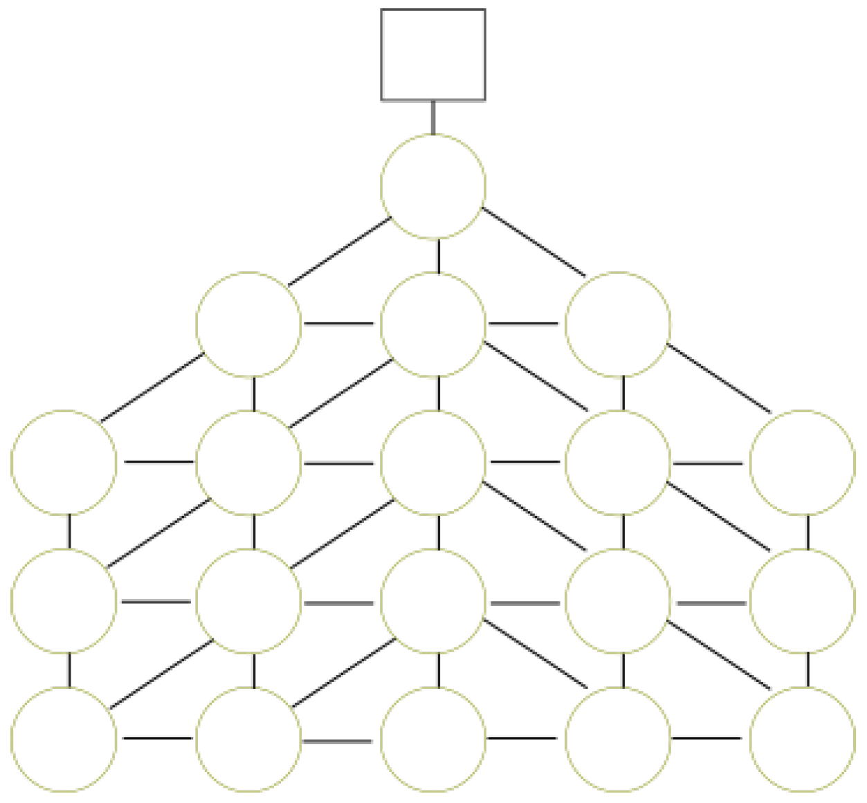Figure 3 shows an example with a DFG $G_3$. For every hexagonal cell, a node is created. Nodes are related with edges if they share a vertex. Therefore, any node has a maximum of six neighbors.

4.2. Enumerating a Data Foraging Graph

To identify the nodes in a unique way, it is necessary to label the graph with numbers. There are many ways to enumerate the nodes of a DFG. Our approach is based on the previously defined representation:

• The root of the graph (base station) is numbered as 0. The next node to be numbered is chosen from a clockwise spiral, as shown in Figure 4.
• The process stops when all nodes of the DFG are numbered.

This approach is used because it simplifies comprehension and readability of the DFG.

4.3. Data Foraging Graph Properties

The properties of any given DFG $G_h$ of size h are introduced. The properties help us formally define the problem of Data Foraging-Oriented Reconnaissance (DFORE) for any Hextille of radius $h_{ex}$ and analyze our algorithm to prove it satisfies the restrictions of DFORE.

The linear distance between the base station and the farthest region is called the depth of the DFG.

Property 1.

For any given DFG $G_h$ where $h\ge 1$, its depth $p_h$ is equal to:

$$p_h=2h-1.$$

(1)

To show that Property 1 a straight line is drawn from the base station of $G_h$ to the farthest node of the graph and count the number of regions the lines cross are counted.

The hexagonal tilling consists of a number of hexagons bordered by other hexagons. It is necessary to know the number of hexagons for any Hextille with radius $h_{ex}$. This allows us to know how the sampling area grows and to measure the performance of our algorithm compared to others, in terms of the number of regions they visit. The DFG will also have the same number of nodes as the Hextille.

Property 2.

For any given DFG $G_h$ with depth $p_h$ (see Equation (1)), the number of regions $n_h$ is given by the following recursion:

$$n_h=(3p_{h-1}+3)+n_{h-1}$$

The close solution for the recurrence is (see Appendix A):

$$n_h=3h^2-3h+1$$

(2)

The focus is on the minimum number of steps to travel from the base station to another region of the DFG without having to recharge the MDF.

Property 3.

Let ${ϵ}_h$ be the required number of steps that are necessary to reach any region from the base station. For any DFG $G_h$, $h\ge 1$, the required number of steps ${ϵ}_h$ is:

$${ϵ}_h=2h-1.$$

(3)

Since it is necessary to return to the base station, the total number of steps an MDF can make is $2{ϵ}_h$.

Property 4.

Let η be the farthest region from the base within the main line. Let ζ be the base station, which is at the root of the DFG.

It is impossible to get from one region to all the regions of the DFG with the movement capabilities of the MDF. Only the base station can be reached from any region of the DFG with the required number of steps (see Property 3). Therefore, we are interested in defining the set of reachable regions given the remaining energy of the MDF.

Property 5.

Let be two regions, $r,r^{\prime }\in R,r\ne r^{\prime }$, the remaining number of steps $e_u$ of an MDF and the physical distance between a pair of regions r and $r^{\prime }$ noted as $d(r,r^{\prime })$. A region $r^{\prime }$ is reachable if and only if there are enough steps Π to visit the region and return to the base station:

$$\mathrm{\Pi }=e_u-d(r,r^{\prime })-d(r^{\prime },\zeta )\ge 0$$

(4)

4.4. Problem Definition According to Our Environment Representation

With our environment representation, the problem of Data Foraging-Oriented Reconnaissance (DFORE) can be formally defined using the previously defined properties.

DFORE: The objective of DFORE is to stamp every region in the sampling area, while visiting nodes according to their priority. This will ensure that the algorithm obtains points of attraction based on trip overlaps. Each MDF will stamp regions by retrieving data from the region. Formally, the problem of DFORE must meet the following restrictions:

Restriction 1.

Every region in the sampling area must be visited and stamped with a pheromone before a maximum time. Let $Tstart$ be the reconnaissance’s start time, $Tstam{p}_t\left(r\right)$ be the time of the visit and stamping of a region $r\in R$ with a pheromone f in the set F at step t, related to the number of regions visited since $Tstart$. Finally, let $T_{expMax}$ be the maximum reconnaissance time, the reconnaissance step must meet:

$$\forall r\in R,\left|Tstam{p}_t\left(r\right)-Tstart\right|\le T_{expMax}$$

(5)

Restriction 2.

Every MDF must return to the base station ζ within its specified maximum endurance. Let $e_u$ be the endurance of an MDF u

$$Tstam{p}_t\left(\zeta \right)\le e_u.$$

(6)

Restriction 3.

Continuity: Every move of an MDF must be done only on adjacent regions. That is, an MDF cannot jump from one region to another one which is not adjacent to it.

Restriction 4.

Interruptibility: The MDF must return to the base station ζ in at most $2{ϵ}_h$ steps, where ${ϵ}_h$ is the required number of steps to arrive from the base station ζ to the farthest region η.

4.5. Proposed Algorithm

At the beginning of the mission, there is no information about the sampling area. After Hextille H with radius $h_{ex}$ is selected, we construct a DFG $G_h$ of the sampling area and explore it. Once the MDF has visited a region in $G_h$, the MDF stamps the region. The objective of reconnaissance is to expand the knowledge of the sampling area while visiting nodes based on their priority. In order to explore new nodes getting to farthest and less stamped nodes is preferred. It is necessary to satisfy Restrictions 2, 3 and 4 (see Section 4.4). The following rules are:

Rule 1.

Given the remaining energy $e_u$ of an MDF, the set of potential nodes $L_r$, the minimum number of steps ${ϵ}_h$ to traverse the DFG $G_h$, a region r, its neighbors $V_r$, the next potential node $r^{\prime }$ to be visited by an MDF is a $r^{\prime }\in L_r\subseteq V_r$. The set $L_r$ is determined by:

• (a) if $e_u>{ϵ}_h$, $L_r\leftarrow$ {$r^{\prime }\in V_r$ : $d(r^{\prime },\zeta )\ge d(r^{″},\zeta )\forall r^{″}\in V_r$},
• (b) otherwise, $L_r\leftarrow$ {$r^{\prime }\in V_r$ : $d(r^{\prime },\zeta )\le d(r^{″},\zeta )\forall r^{″}\in V_r$ }.

Rule 2.

Given a region r and its neighbors $L_r$, an MDF can only move if $\exists r^{\prime }\in L_r$ such that the estimated remaining energy between r and $r^{\prime }$, $\mathrm{\Pi }\ge 0$ (see Property 5).

The rules are implemented in the algorithm. The main function of the algorithm is shown in Algorithm 1. The detailed description of the DFORE algorithm is presented in Appendix D.

Algorithm 1 Exploration algorithm.

1: function [List<Cell>, int] exploration(int $e_u$, List<Cell> $area$) 2:  int $time\leftarrow 0$ 3:  Cell $r\leftarrow 0$ 4:  while $e_u\ge$ 0 do 5:   if $(e_u-2)-e_{base}$- ≥ 0 then 6:    Cell $r^{\prime }\leftarrow$ choose(neighbors(r)) /* See Appendix D */ 7:   else 8:    Cell $r^{\prime }\leftarrow$ traceback(neighbors(r), $e_u$) /* See Appendix D */ 9:   end if 10:   $e_u^{\prime }\leftarrow e_u-1$ 11:   $r^{\prime }.stamp\leftarrow r^{\prime }.stamp+1$ 12:   $tim{e}^{\prime }\leftarrow time+1$ 13:   $r\leftarrow r^{\prime }$ 14:  end while 15:  $List<Cell>foodCells\leftarrow$ getFoodCells($area$) /* See Appendix D */ 16:  return $[foodCells,time]$ 17: end function

Next, the DFORE algorithm is described. If the environment has not been visited completely, the reconnaissance continues its execution while the MDF has enough number of steps to continue exploring the DFG. In order to choose the next node to be visited, it is necessary to verify whether the MDF has enough remaining steps to proceed (function EXPLORATION line 4, Rule 2) or needs to return (function EXPLORATION line 6). If the MDF can proceed, the following heuristics are applied. First, the MDF selects the adjacent nodes with the largest distance to the base station $\zeta$ (see Rule 1a). Second, the MDF chooses the nodes with fewer stamps (function choose see Appendix D line 6). Third, if all conditions hold, i.e., every node has the same distance to the base station and the nodes have the same number of stamps, then the MDF chooses a node at random with a uniform distribution (function choose see Appendix D line 7). After moving to the last node, the MDF must return to recharge energy. 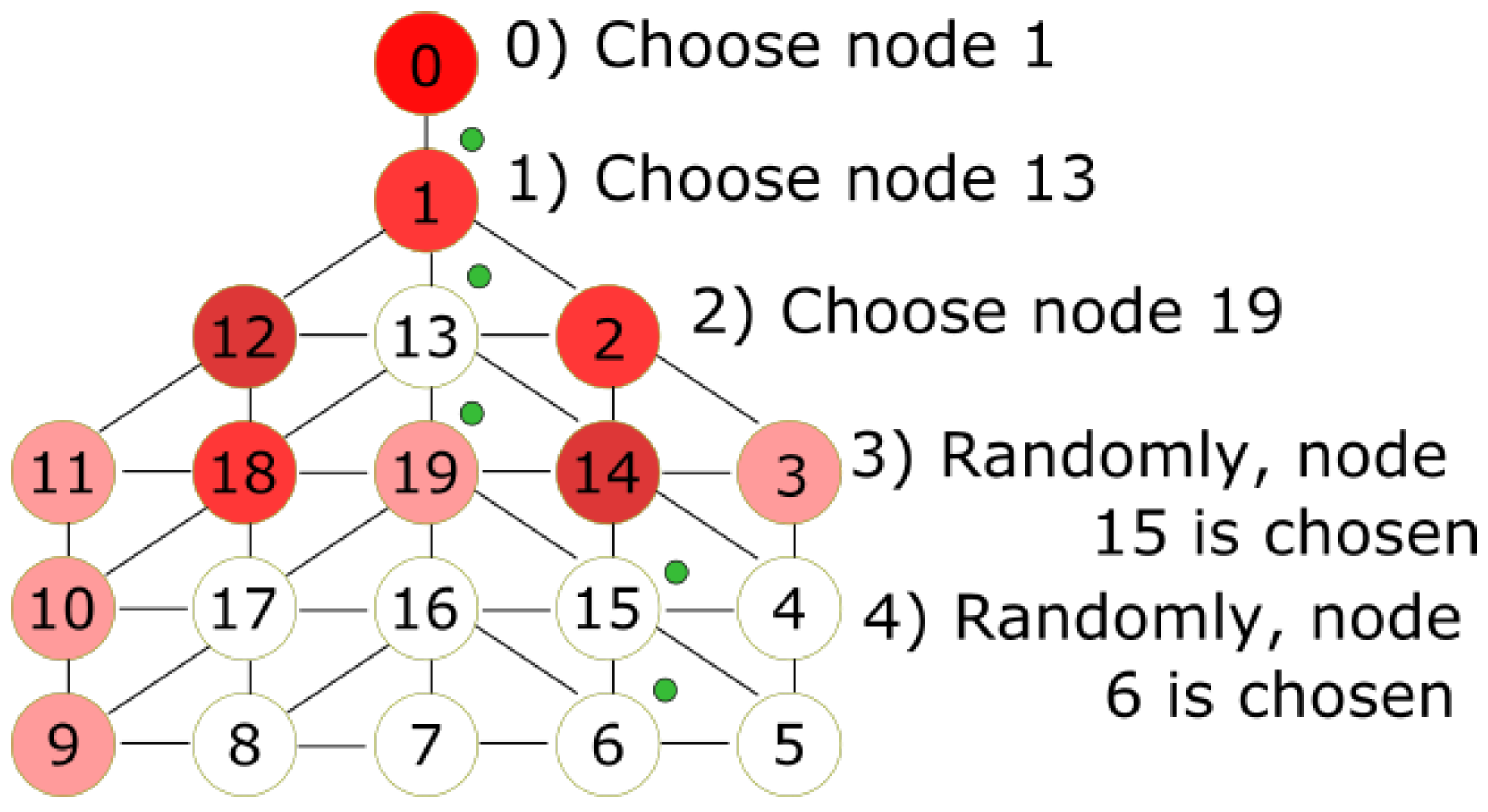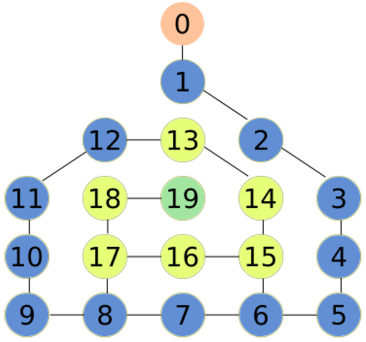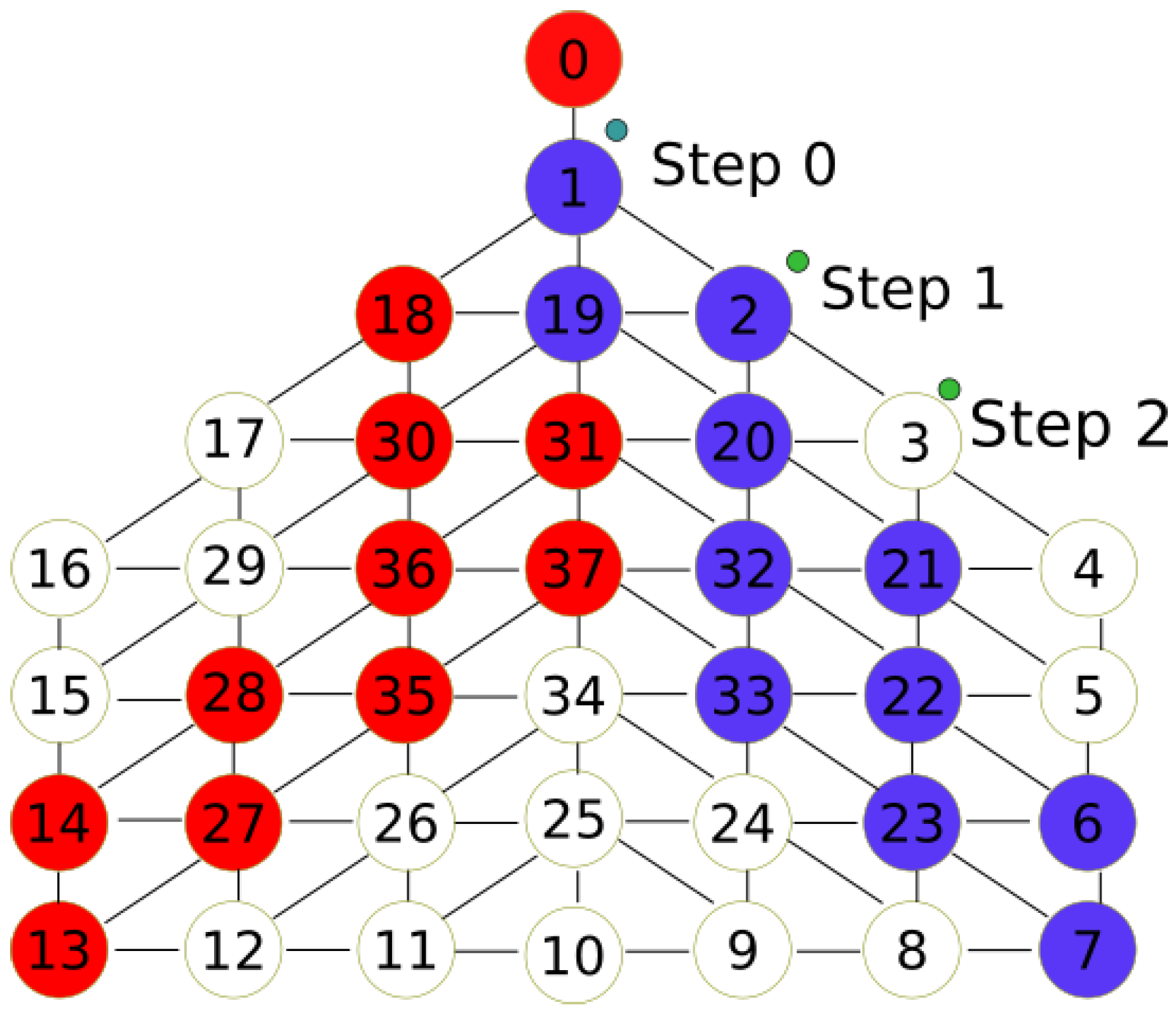Thus, when the MDF cannot proceed, then it will begin to choose nodes which are nearer to the base station (see Rule 1b); therefore, the MDF will return to the base station satisfying Restriction 4 (see Section 4.4). 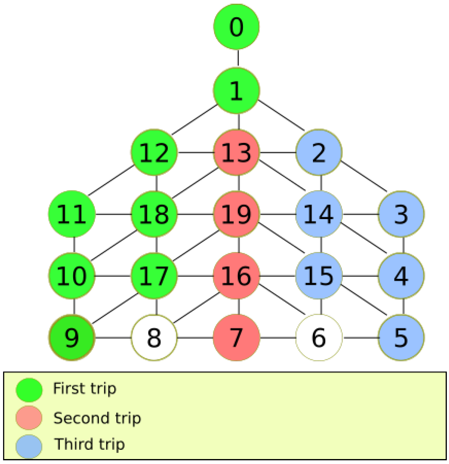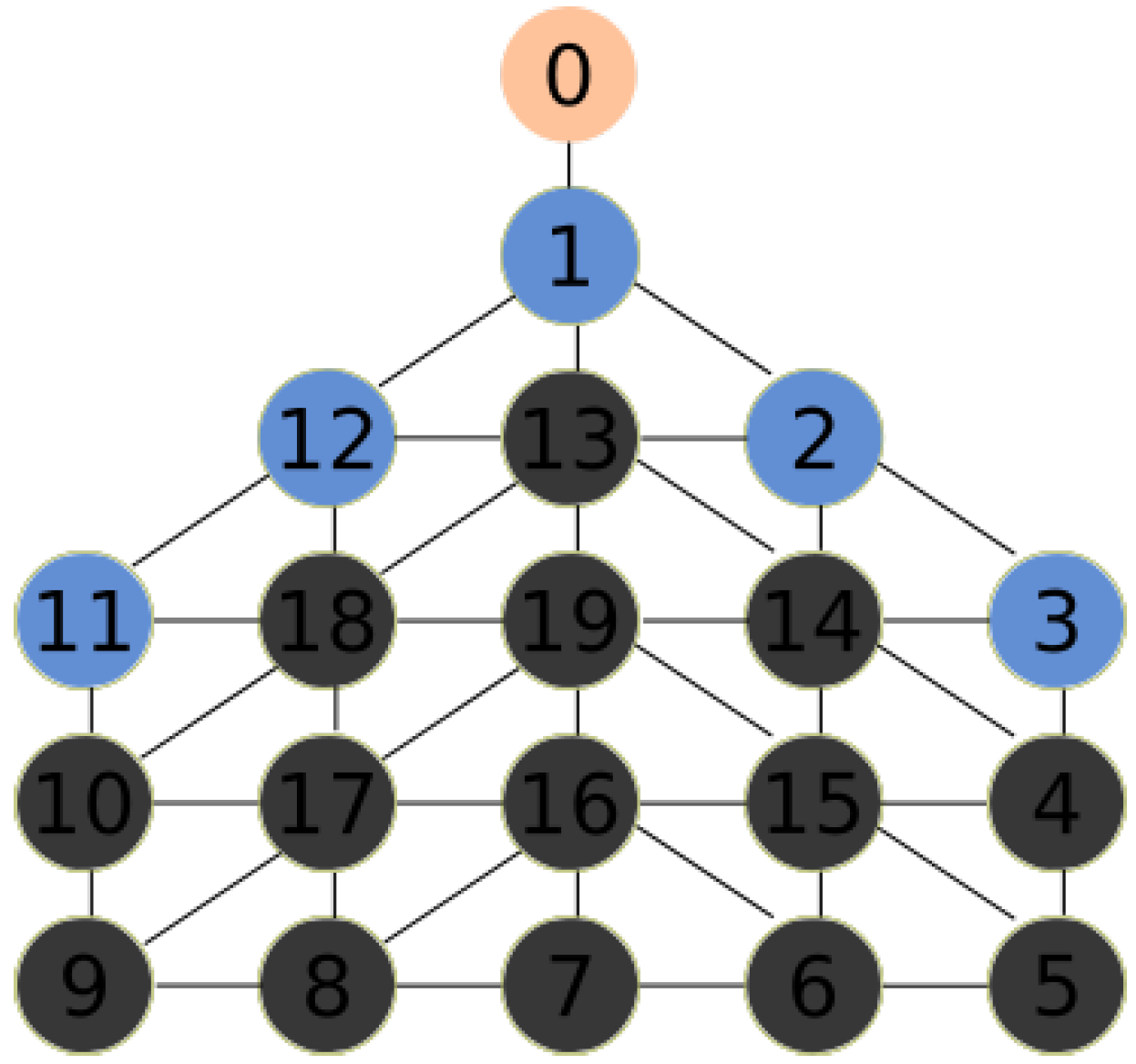See Figure 5 for the following example. All red nodes are stamped, the number of stamps is represented by the intensity of the color. The MDF is currently on node 0. At step 0, the MDF chooses node 1 since it has only one choice. At step 1, the MDF chooses node 13, which is not stamped. Node 19 with less stamps is chosen at step 2. The MDF chooses randomly node 15 at step 3. In step 4, the MDF chooses node at random.

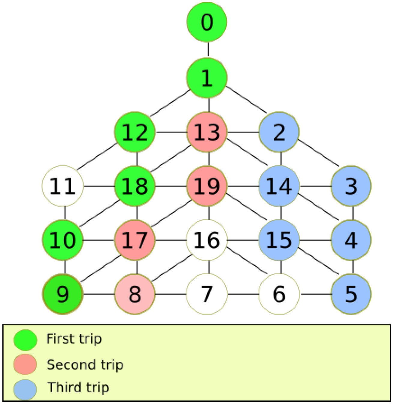
To show an example of the execution of our algorithm in various trips, Figure 6 depicts an example of the reconnaissance algorithm for a DFG $G_3$. Each color represents the trip taken. Uncolored nodes are not visited yet. The first trip is colored in green. When the MDF cannot proceed, it returns to recharge energy at the base station. In the second trip, the MDF explores unvisited nodes, puts a pink stamp and returns. Finally, in the last trip, the MDF visits another group of nodes and paints them blue. In order to explore the entire graph, overlaps between trips must occur. It can be noted that in the last trip, the MDF exploits better the movement capabilities since it explores more nodes in one trip.

5. Algorithm Analysis

In this section, the mathematical analysis of our algorithm is discussed to show that it satisfies the restrictions of the problem. The number of trips required to explore any DFG with n regions is analyzed. The first part is devoted to the use of the required number of steps ${ϵ}_h$ to traverse the whole DFG, both in the best and in the general case of reconnaissance. Based on this analysis, the minimum and expected number of trips for any DFG with n regions is obtained. Finally, the number of trips required to visit every node in the DFG is analyzed with a greater number of steps than ${ϵ}_h$.

5.1. Number of Trips Using the Required Number of Steps: Best Case

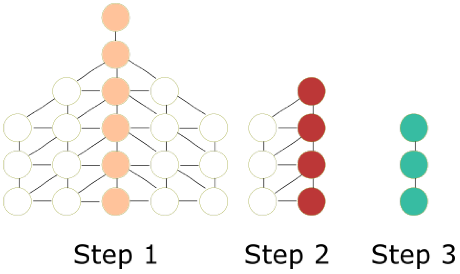
The best case occurs when there is almost no overlap of paths to visit every node in the DFG. If the graph $G_h$ is divided by a straight line between the base station and the farthest region $\eta$, symmetrical sub areas are obtained. Figure 7 shows the environment divided in half. If the process continues, eventually only a straight line is obtained. Thus, it is possible to apply a divide and conquer strategy. Formally, this behavior is defined as follows. Let f(n) be the problem of exploring an environment represented by graph G with n regions.

Definition 1.

Each time the DFG $G_h$ is divided, f(n) is split into two equal subsets with the same cardinality. In order to combine the solution, at least n steps need to move towards the base station. Therefore, for any given environment $f\left(n\right)$ can be expressed by:

$$f\left(n\right)=2f(n/2)+c$$

(7)

where c is a constant.

We have a linear time to explore n nodes, that is: $f\left(n\right)=\mathcal{O}\left(n\right)$ (see Appendix B). However, there is a precise way of calculating the minimum number of trips required to explore any DFG $G_h$, given the required number of steps ${ϵ}_h$ available. There are two ways that a main line can be traversed: Either by choosing a main line and returning to the base using the same regions, or by backtracking using the next row of regions. However, the farthest region $\eta$ of the next row will not be marked. Figure 8 shows an example of this situation. It can be seen that the minimum number of trips for any given DFG $G_h$ is equal to its depth $p_h$.

Definition 2.

The minimum number of trips $T_h$ to explore any given DFG $G_h$ is equal to its depth $p_h$ (see Equation (1)).

$$T_h=p_h$$

(8)

For any DFG $G_h$, in every trip, the number of nodes traversed is $2(2h-1)$. Since there are $T_h$ trips, the total number of nodes traversed required to explore the DFG $G_h$ is $2T_h(2h-1)$. Based on Equation (8), the previous equation is $2{(2h-1)}^2$. Expanding the equation yields:    

$$f\left(n\right)=8h^2-8h+2$$

(9)

However, to obtain profitable data sources, various trips must overlap in order to discriminate valuable sources from common ones. Therefore, a general case of reconnaissance where various trips overlap must be addressed.

5.2. Number of Trips Using the Required Number of Steps: General Case

In the general case, the interest is to visit several nodes repeatedly in order to obtain valuable nodes, contrary to the goal in the best case. Therefore, the focus is to obtain the average number of trips to explore the DFG considering the heuristics of our proposal. In order to calculate the average number of trips, the environment is divided into rows and columns. The rows correspond to the levels in the graph while the columns are represented by the width of the graph. This division is shown in Figure 9. The columns correspond to the blue nodes, and the levels start at the base station. Only the blue nodes are considered because if a blue node is visited, there is a chance to visit all the nodes in the column due to the heuristics of the proposed solution. For example, if the current node is 3, the MDF will choose 4 over 14 and 2 because the distance from 4 to the base station is greater than all the adjacent nodes of the current node.

Since there are many possibilities to travel in the blue nodes, it is necessary to calculate the number of trips on average to stamp every node in the column.

Table 2. Average trips to cover all the siblings on the line of each blue node.

Node	Average Ways
1	9
2	4
3	1
12	4
11	1

shows the average ways we need to pass by each blue node in order to stamp every node in that column. The first column of Table 2 contains each blue node, and the second column presents the average number of ways a particular blue node can have all its siblings visited based on the DFORE algorithm. The number of average trips is the number of edges the MDF can take from a blue node using the heuristics of the algorithm. For example, for the blue node 2, there are four possible edges. The first edge is in the line that consists of nodes {14, 15, 6}; the second edge is from node 2 to 3; the third edge is from 14 to 4; and the last edge is from 15 to 5. There is not an edge between 6 and 5 since it is impossible to get from 6 to 5 with the required number of steps. Therefore, the number of edges of all blue nodes is the average number of trips required to explore the graph. We show the equation of the expected number of trips for any given DFG.

Definition 3.

Given a DFG $G_h$ with depth $p_h$ (see Equation (1)). The expected average number of trips $T_h$ is:

$$T_h=2p_h+2\sum _{j=1}^{h-2}(p_h-j)+1.$$

(10)

However, there is a simpler way to calculate the expected average number of trips for any given DFG. To obtain the expression, a table for each environment is built.

Table 3. Variables for each environment.

DFG size h	Number of nodes ${\mathit{n}}_{\mathit{h}}$	Depth of ${\mathit{G}}_{\mathit{h}}$	${\mathit{n}}_{\mathit{h}}-{\mathit{n}}_{\mathit{h}-1}$
1	1	1
2	7	3	6
3	19	5	12
4	37	7	18
5	61	9	24
6	91	11	30
7	127	13	36
8	169	15	42
9	217	17	48
10	271	19	54
11	331	21	60

shows each DFG $G_h$ with the correspondent variables. In the first column, the size of each DFG is shown. The second column contains the number of nodes in each DFG. The third column shows the depth of the graphs. Finally, the difference between the number of nodes of DFG of size h and $h-1$ is presented in the last column. We note that each successive environment grows by a fixed amount of six as shown in the last row of the table. For example, with the DFG $G_3$, the number of nodes is 19, while for the DFG it is 7, and their difference is 19 − 7, which is equal to 12.

Taking into consideration the growth of each successive Hextille, the number of regions for any Hextille is given by the following expression: $n_h=3h^2-3h+1$ (see Appendix B). Finally, the expected average number of trips is $T_h=3h^2-3h+1$ (see Appendix A). Therefore, $T_h=n_h$.

Furthermore, to get the computational cost of the general case, consider that the number of nodes visited by each trip is $2{ϵ}_h$. Therefore, if there are $T_h$ trips, the total number of nodes is $2T_h{ϵ}_h$. Since $T_h=n_h$, the expression is $2n_h{ϵ}_h$. Also, notice that $n_h>2{ϵ}_h$. Since $2{ϵ}_h$ is a constant, we ignore it. Thus, the general case of exploration is linear $\mathcal{O}\left(n\right)$ with respect to the number of nodes in any DFG.

We have calculated the average number of trips for any DFG with the required number of steps ${ϵ}_h$. When the number of steps of the MDF $e_u$ is bigger than the required number of steps ${ϵ}_h$ of a given DFG $G_h$, that is $e_u>{ϵ}_h$, the number of regions visited is increased by a constant factor. Therefore, the expected number of trips remains the same; thus, the reconnaissance time is linear with respect to the number of nodes visited: $f\left(n\right)\subseteq \mathcal{O}\left(n\right)$.

6. Correctness Proof

Section 5 shows that our algorithm has a linear time $\mathcal{O}\left(n\right)$ while the upper bound of exploration under interruption is $\mathcal{O}\left(n^2\right)$. Now we prove that our proposal satisfies the DFORE’s restrictions. Reconnaissance must satisfy the following restriction: $\forall r\in R,\left|Tstam{p}_t\left(r\right)-Tstart\right|\le T_{expMax}$ (see Section 4.4). The maximum reconnaissance time for any given DFG $G_h$ where $i\in$ $\mathbb{N}$ under interruptibility is $n_h^2$. This is the time needed to explore the graph using DFS [17]. If the reconnaissance time of our proposed algorithm is greater than $n_h^2$, then it is not better than DFS, and therefore, our proposed algorithm does not satisfy the restriction of the DFORE problem. For this particular proof, we define the reconnaissance time of our algorithm as the sum of the differences between each stamp of a region with respect to the start time $Tstart$, in other words, the time taken by our algorithm to stamp every region in $G_h$. By definition, the stamping time at time t is equal to: $Tstam{p}_t\left(r\right)=Tstam{p}_{t-1}\left(r^{\prime }\right)+t$ where $r\ne r^{\prime }$ and $Tstam{p}_0\left(\zeta \right)=Tstart$.

Definition 4.

For a DFG $G_h$ the number of nodes is $n_h=3h^2-3h+1$; therefore, the reconnaissance time $T_{expMax}$ is equal to:

$$T_{expMax}={(3h^2-3h+1)}^2.$$

(11)

The following restriction should be satisfied:

Restriction 5.

The reconnaissance time of our algorithm $T_{expAlgorithm}$ is less than the maximum reconnaissance time: $T_{expAlgorithm}<$ $T_{expMax}$.

In order to satisfy Restriction 1, the whole area should be explored within the given time $T_{expMax}$. Therefore, both the best and general case must be analyzed. The following theorems state that our algorithm satisfies Restriction 5.

Theorem 1.

The divide and conquer reconnaissance algorithm for the best case satisfies Restriction 5 for any given DFG $G_h$.

Theorem 2.

The reconnaissance algorithm for the general case satisfies Restriction 5 for any given DFG $G_h$.

To prove Theorem 1, the time taken by the reconnaissance step and the time to sample the entire area are calculated. According to Definition 4, the reconnaissance time for any given DFG $G_h$ is $T_{expMax}$ = ${(3h^2-3h+1)}^2$. The time it takes to explore $G_h$ is calculated using the divide and conquer method $T_{expDivide}$ which is equal to $T_{expAlgorithm}$. We know that $T_{expDivide}$ = $2{ϵ}_h{p}_h$ (see Section 5.1). The depth of any given DFG $G_h$ where $h\in \mathbb{N}$ is $p_h=2h-1$. Therefore, $T_{expDivide}$ = 2(${ϵ}_h{)}^2$. To prove that $T_{expMax}$ > $T_{expDivide}$, analyzing the inequality:

$${(3h^2-3h+1)}^2>2{\left({ϵ}_h\right)}^2$$

(12)

$$(9h^4-18h^3+15h^2-6h+1)>(8h^2-8h+2)$$

(13)

The inequation holds if the DFG is greater than one; therefore, $T_{expMax}$ > $T_{expDivide}$ if $h>1$.

Now, the general case for Theorem 2 is proven. Based on the analysis, the average number of trips is $T_h=3h^2-3h+1$. Since every trip takes $2{ϵ}_h$ of steps, the average reconnaissance time $T_{expAlgorithm}$ is: $2T_h{ϵ}_h$. It is necessary to verify that $T_{expAlgorithm}<T_{expMax}$:

$$\begin{array}{c}\hfill \begin{array}{c}\hfill T_{expMax}>T_{expAlgorithm}\\ \hfill 2{\left(T_h\right)}^2>2T_h{ϵ}_h\\ \hfill T_h>{ϵ}_h\\ \hfill 3h^2-3h+1{>}^2(2h-1)\\ \hfill 3h^2-3h+1{>}^{4}h-2\\ \hfill T_{expMax}>T_{expAlgorithm}|h>2\end{array}\end{array}$$

(14)

We have proved that both the best and the general case of our algorithm, for any given DFG, satisfies DFORE’s restrictions. In the following section, our theoretical results are compared with the experimental values.

7. Experiments

To determine the performance of our algorithm under various conditions, two experiments were defined.

In the first experiment, the movement range of the MDF was set between ${ϵ}_h$ and $2{ϵ}_h$ to measure the average number of trips required to place a pheromone in every node of the DFG. The second experiment compares the performance of the DFORE algorithm versus the one obtained by MULES [10], adapted to the foraging reconnaissance task. The comparison with MULES is justified since this proposal is the baseline algorithm for indirect communication among mobile sensors.

7.1. Simulation Versus Theoretical Value

This experiment is conducted in two phases. The first phase is to determine the difference between the average number of simulated trips versus the theoretical bound. In the second phase, the experiments are validated through statistical inference.

7.1.1. Experimental Setup

This experiment includes 5,000,000 flights since the number of simulations provided sufficient data to measure the average number of trips, such that the difference among several simulations was not significant. To determine if the proposed algorithm accomplishes the constraint on the average number of trips given by $T_h=2p_h+2{\sum }_{i=1}^{h-2}(p_h-i)+1$, the number of trips required to travel every DFG $G_h$ were measured. The number of steps was set in the range of $\left[{ϵ}_h,2{ϵ}_h\right]$, with increments of two units, since a unitary increment does not change the behavior of the algorithm due to Restriction 2 (see Section 4.4).

Table 4. Average number of trips per DFGs with our algorithm.

DFG Depth h	AVG Trips	Std. Deviation	Variance	Max	Min
2	3.8890	0.8315	0.6915	5	3
3	10.6992	2.9336	8.6060	32	5
4	19.7592	5.3702	28.8388	59	7
5	33.2963	9.2975	86.4443	114	11

shows the results of this experiment.

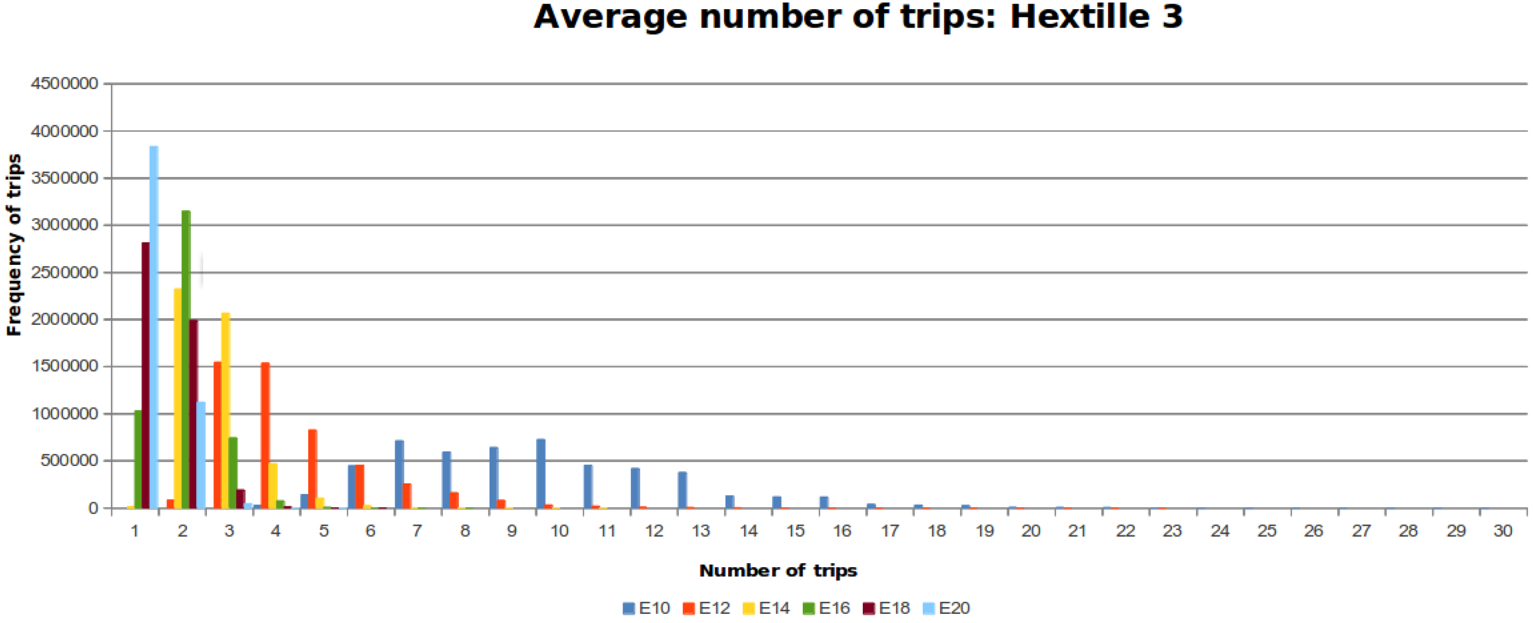
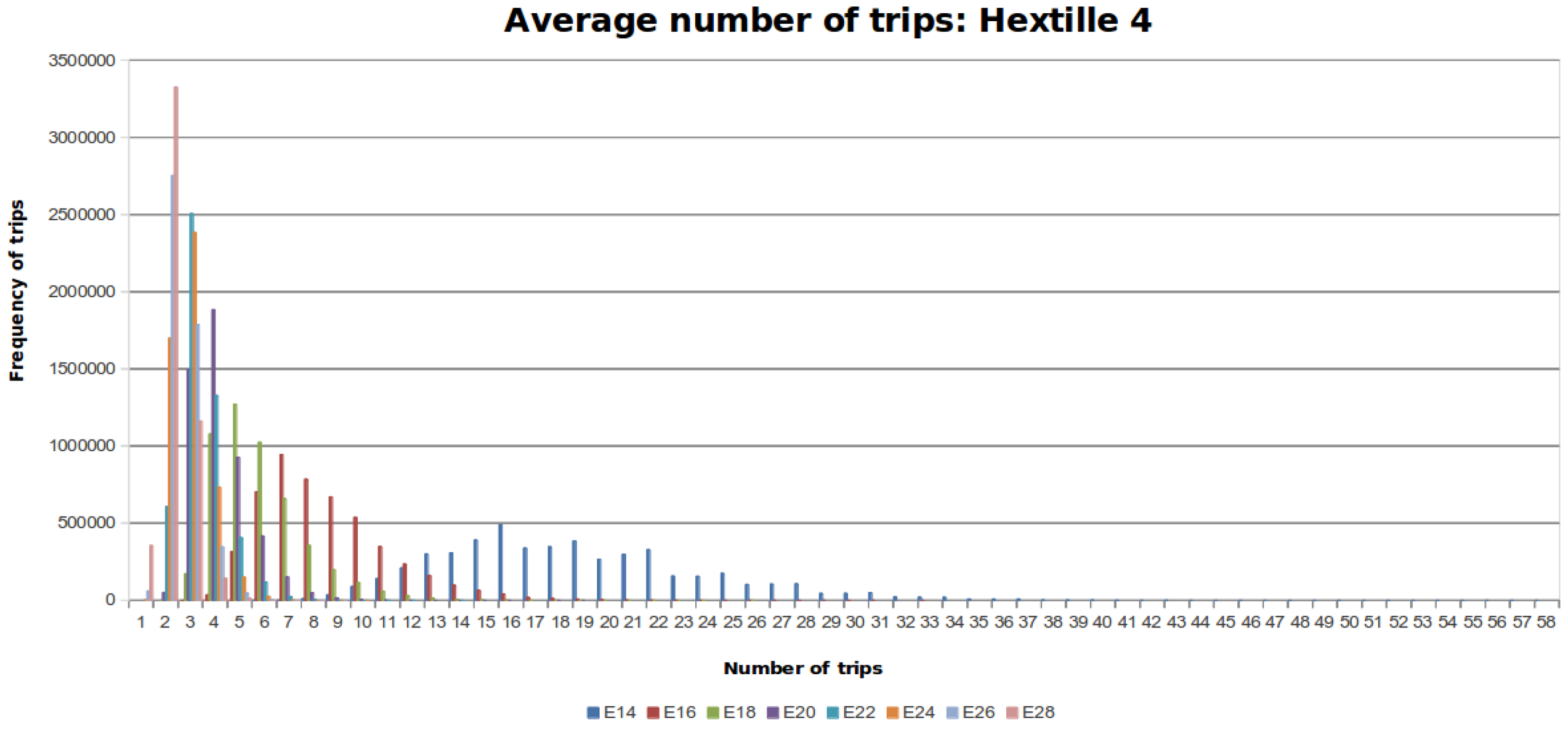
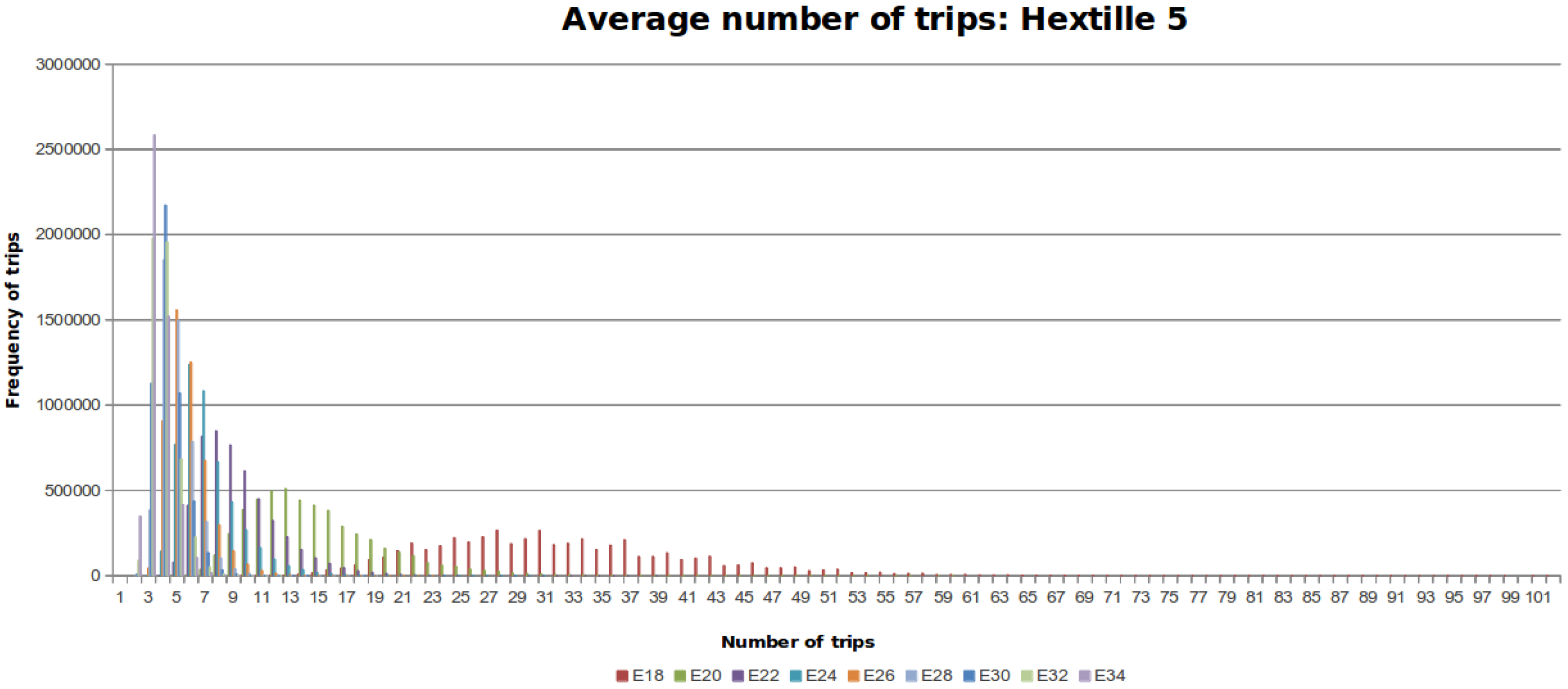
Figure 10, Figure 11 and Figure 12 show the distribution of trips for every DFG considering the different number of steps that the MDF can make. Each colored line represents a histogram with the corresponding trips per steps. The required steps ${ϵ}_h$ to traverse $G_h$ is colored blue. When the number of steps increases by a factor of two, the data distribution is skewed towards the left around a peak value.

7.1.2. Statistical Inference

A statistical inference test was done to prove that the average number of trips performed by the proposed algorithm is different from the theoretical value $T_h$. For this, 50 random samples of flights were taken, as statistical sample, for every DFG. We define the null hypothesis $H_0$ as: the average number of trips θ is equal to $T_h$ and the alternative hypothesis $H_1$ as: the average number of trips θ is less than $T_h$. Considering the p-value obtained from each set of experiments, the null hypothesis is rejected with a $95\%$ level of confidence, as it can be seen in

Table 5. T-statistics for each DFGs $G_3,G_4,G_5$ with the samples. For each row, we have tested $H_0$ against the results.

DFG Depth h	AVG Trips	T-Statistic	p-Value	${\mathit{H}}_0$
3	10.8	6.82	<0.00001	Reject
4	20.9	4.01	0.002289	Reject
5	33.37	2.84	0.005388	Reject

.

A t-test is applied since we obtain a normal distribution due to the randomness of the movements performed in the experiments. In addition, due to the size of the sample, the variance between trips is homogeneous and there are no significant outliers.

Table 6. Average trips per DFGs $G_3,G_4,G_5$ taken from a sample of 50 random flights.

DFG Depth h	AVG Trips	Std. Deviation	Variance	${\mathit{T}}_{\mathit{h}}$
3	10.8	3.0017	9.0101	19
4	20.9	6.3365	40.1515	37
5	33.37	8.7532	76.6193	61

shows the statistic test. Since the significance level $\alpha$ is 0.05, for every DFG $G_h$ the test passed.

7.2. DFORE Compared with MULES Reconnaissance

In this section the DFORE algorithm is compared with MULES. The MDF starts at the base station both for the DFORE algorithm and MULES. The MDF explores the whole environment using the two algorithms in different experiments, measuring the average number of trips performed by each one over DFGs $G_3,G_4$. In this way, considering a sample of 10,000 flights, the difference between the average number of visited regions by each algorithm was measured.

We define the null hypothesis $H_0$ as: there is no significant difference between MULES [10] and our proposed algorithm, i.e., the average number of trips $\theta$ of MULES is not different from the average number of trips $\vartheta$ of our proposed algorithm. The alternative hypothesis $H_1$ is: there is a significant difference between θ and ϑ. The null hypothesis is rejected with a $95\%$ level of confidence.

Table 7. Results of our proposed algorithm compared with MULE for DFGs $G_h$ of size h = (2, 3, 4).

Algorithm	AVG Trips	Std. Deviation	Variance	Max	Min
Proposed alg. $G_2$	3.8922	0.8326	0.6933	5	3
MULES $G_2$	13.7152	10.5584	111.4790	122	3
Proposed alg. $G_3$	10.6784	2.9283	8.5751	26	5
MULES $G_3$	206.6570	181.1481	32,814.6230	2290	6
Proposed alg. $G_4$	19.7463	5.3766	28.9077	54	7
MULES $G_4$	3189.4170	2981.9314	8,891,914.6828	33730	66

shows the results of this experiment. There is a clear difference between the average number of trips of the two algorithms. The proposed algorithm has a better performance than MULES, since it performs less trips than MULES.

8. Discussion

Based on the results obtained from the experiments two facts are concluded. First, the data obtained shows that the average number of trips falls within the mathematical bound obtained theoretically. From Figure 10, Figure 11 and Figure 12, it can be seen that the data follows a distribution towards the mean, despite the randomness part of our proposed algorithm. In addition, if the movement capabilities are increased by two units, the number of trips decreases, as shown in Figure 12. Furthermore, based on the results of the second experiment (see Section 7.2), we have evidence that our algorithm has better performance than MULES [10]. This is explained by the random movement of MULES against the oriented movement of our proposed algorithm. The orientation towards unexplored regions is done through indirect communication using the artificial pheromones segregated by each mobile sensor in the regions. Therefore, the average number of trips required to deposit at least one pheromone in all the graph using our proposed algorithm is less than that of MULES. The trade-off between computational time and run time of the algorithm is shown in a comparison between a random walk algorithm, such as Data MULES, and our proposed algorithm.

9. Conclusions

We have presented a data-foraging-oriented reconnaissance algorithm based on bio-inspired indirect communication for aerial vehicles. One original contribution is the definition of an artificial pheromone, as an abstract data type, oriented to perform stigmergy-based communications. Through the virtual segregation of such pheromones, the algorithm allows aerial vehicles which sense a given area, to communicate indirectly their findings. In this way, aerial vehicles can create several paths oriented to explore the environment and recognize profitable data sources. By considering the energy constraints of aerial vehicles and their impact on their movement capabilities, the operational environment was discretized in the form of a set of regions organized into a Hextille. Then, based on the Hextille, the environment is formally modeled as a connected undirected graph called Data Foraging Graph (DFG). The artificial pheromones segregated are related to an area that is the region visited, which corresponds to a node in the DFG. The Data Foraging-Oriented Reconnaissance problem has been defined. We identify and define the required and sufficient movement capacity capabilities of the aerial vehicle per trip to explore an environment according to the depth of the DFG. The solution proposed was formally specified and mathematically evaluated. The results prove the viability and efficiency of the solution. Additionally, we have presented a study increasing the aerial vehicle’s movement capability. The results of this study show that the average number of trips and the run time to explore the environment highly decrease as the movement capability increases.