Robust Co-Optimization to Energy and Reserve Joint Dispatch Considering Wind Power Generation and Zonal Reserve Constraints in Real-Time Electricity Markets

Abstract

This paper proposes an energy and reserve joint dispatch model based on a robust optimization approach in real-time electricity markets, considering wind power generation uncertainties as well as zonal reserve constraints under both normal and N-1 contingency conditions. In the proposed model, the operating reserves are classified as regulating reserve and spinning reserve according to the response performance. More specifically, the regulating reserve is usually utilized to reduce the gap due to forecasting errors, while the spinning reserve is commonly adopted to enhance the ability for N-1 contingencies. Since the transmission bottlenecks may inhibit the deliverability of reserve, the zonal placement of spinning reserve is considered in this paper to improve the reserve deliverability under the contingencies. Numerical results on the IEEE 118-bus test system show the effectiveness of the proposed model.

1. Introduction

To alleviate the problem of fossil energy shortages, excessive carbon emissions, and ecological damages, power generation based on large-scale renewables like wind and solar photovoltaic has been developed at a rapid rate. However, uncertainties related to renewable energies bring negative effects to the operation and to the dispatch of the entire power system, such as real-time power balance, load flow of transmission lines and the optimal placement of reserve capacity.

In order to address the issue of uncertainties in renewable energy outputs, robust optimization methods have been explored widely. Major strong points of those robust optimization methods include:

(1)

An accurate probability distribution function of the uncertain parameters such as the wind power output, which is usually difficult to obtain and may lead to model insolubility [1], is not required;

(2)

Solutions are feasible even when the worst cases occur in practice [2];

(3)

With proper mathematical treatments of the robust model, the computational tractability can be realized [3].

Generally, robust optimization methods can be adopted in wind power system analysis for various objectives. One is to determine the base point of the generation output while satisfying the power balance for all possible wind power outputs, followed by the computation of participation factors, which is an effective solution for the penetration of wind power into the power system [4]. In addition, a robust co-optimization to energy and ancillary service joint dispatch considering wind power uncertainties in real-time electricity markets was proposed in [5]. Both models in [4,5] are based on Direct Current (DC) power flow. Therefore, the participation factors employed in those papers to produce adjustable generation outputs immune to uncertain wind power generation and the robust optimization model can be equivalently transformed into a linear programming model. There are also other discussions on robust optimization models in [6,7,8]. For example, the robust scheduling of traditional thermal power plant outputs with wind power generation to match the uncertain load demand can be formulated as a robust shortest path problem (RSSP) [6]. Moreover, to address the problem of security constrained unit commitment (SCUC) in the presence of uncertain active power injection of wind power generation, a two-stage adaptive robust unit commitment model was built up in [7]. Furthermore, a practical solution method based on Benders decomposition type algorithm was also provided in [7]. An optimal power flow (OPF) model using the Taguchi's orthogonal array testing and probabilistic power flow calculation to achieve a minimized generation cost robust to uncertainties was introduced in [8]. Beyond merely coping with the operation, planning and scheduling problems linked to uncertainties in the power system, robust optimization can also be used in the electricity market. To address a small size electric energy system equipped with smart grid technology as a virtual power plant that can strategically buy and sell energy, a two-stage procedure based on robust optimization was proposed in [9]. Moreover, when a price-taker participates in the pool market, robust optimization can also provide a bidding strategy along with a technique to build hourly offering curves [10]. In addition to the single-period problem, a robust optimization model for wind power look-ahead dispatch, which aims to manage operational uncertainties over the next several hours, has been discussed in [11]. In terms of equipment controlling, robust optimization can also play a vital role. Furthermore, a fractional order automatic generation control (AGC) adjustment based robust optimization techniques is proposed to address the distributed uncertain renewable energies [12]. To control the conservatism of the robust optimization model, [13] focused on accommodating uncertain wind power while avoiding over-protection by the use of risk measure. The total cost is reduced significantly when considering pump-storage units.

However, the above models only studied the optimal dispatch in the energy market but rarely discussed on the ancillary service. As for frequency stability, reserve capacity is required by each generator to deal with uncertainty from wind power generation outputs, as well as temporary outages of generation units. As a result, several types of reserves have been developed and applied in power system to smooth the output of renewable energy in an economically efficient way. Reserves can be classified by their usages as regulating reserve and spinning reserve. Specifically, the regulating reserve is used to balance any instantaneous power mismatch caused by load and generation output fluctuations. In contrast, the spinning reserve is used to compensate the shortage of active power when an outage of a generator occurs. Obviously, the more reserve there is in a power system, the higher its reliability will be. Nevertheless, too much reserve capacity in the generators may lead to a higher cost. Therefore, the question as to how to balance the generation dispatch and reserve capacity is very important.

To deal with this issue, several methods of energy and reserve dispatch were proposed, e.g., a merit order based dispatch method [14], a sequential dispatch method [15], and a joint dispatch approach [16,17,18]. For the methods in [14,15], the energy dispatch and ancillary service dispatch are optimized separately according to their priorities. However, they may be suboptimal or even infeasible, which may result in insufficient supply for the lower priority commodity [16,17]. By contrast, the joint dispatch model presented in [18] is based on a formulation in the context of the constrained optimization model. The normal energy and reserve joint dispatch method usually aims to minimize the total costs of energy and reserve to obtain an economically optimal dispatch schedule, together with a consideration of the equation of power balance, generator ramp rate limits, the constraints of transmission line capacity, and minimum reserve requirements [19]. For this reason, Midcontinent ISO (MISO) has operated in this joint market since 2009, where the energy and reserve dispatch are considered as competitive commodities and then co-optimized in the real-time deregulated market every 5 min [20,21,22]. According to the rule of market mechanism in energy and ancillary markets, references [23,24] presented comprehensive models and pricing mechanisms using the robust co-optimization approach in the day-ahead market and real-time market, respectively.

Note that the reliability and deliverability of energy and reserves are very important. Those should be considered into the optimization model, especially under contingencies when the network congestion is particularly remarkable. Zonal reserve constraints can guarantee the minimum requirement for reserves of each zone to be satisfied, and therefore overcome the problem of network congestion. As a result, the zonal reserve constraints can be incorporated into the conventional security constraints to maintain deliverability of reserves in the system. In [23], the ISO New England market clearing framework for the co-optimized real-time energy-reserve market was discussed, and reserve deliverability for nested reserve zones was recognized. A security-constrained unit commitment model for energy and ancillary services auction was proposed in [24], where reserve requirements are optimized in electricity markets by simulating contingencies rather than specifying the requirements as fixed system constraints.

Furthermore, to manage and increase the integration of renewable energy in the power system, an innovative procedure is needed for both normal and abnormal conditions. In this sense, a model incorporated an N-k security criterion, by which the power balance is guaranteed under any contingency state comprising the simultaneous loss of up to K generation units, was formulated in [25]. In addition, a two-stage robust optimization was provided in [26] considering all possible component failure scenarios including both generator and transmission line contingencies. In the technical literature, the execution of N-k criterion usually costs more time and has therefore a negative impact on solutions efficiency. Moreover, it has not been fully studied. Consequently, the motivation of this paper is to represent the benefits of combining active set method with security constraints to improve the efficiency of N-1 criterion verification.

This paper focuses on the optimal scheduling of active power in the power system with the integration of large-scale wind power generation. The reactive power generation, transmission, and consumption in the system are assumed to be maintained in normal operation. Therefore, the practical engineering DC power flow formulation and algorithm can be employed, resulting in a very efficient computational behavior. Meanwhile, the global optimality and convergence can be strictly guaranteed.

In this paper, a robust co-optimization model is thus set up to find an optimal scheduled generation while guaranteeing the security of the power systems for any given wind power as well as any N-1 contingency of both transmission lines and generators.

Compared with the prior art works, the major contributions of this paper are summarized as:

(1)

The model proposed in this paper can generate a robust scheduling scheme immune to the largest fluctuation of the renewable energy output;

(2)

The zonal spinning reserves can enable the deliverability of spinning reserves, particularly when an outage of generators occurs;

(3)

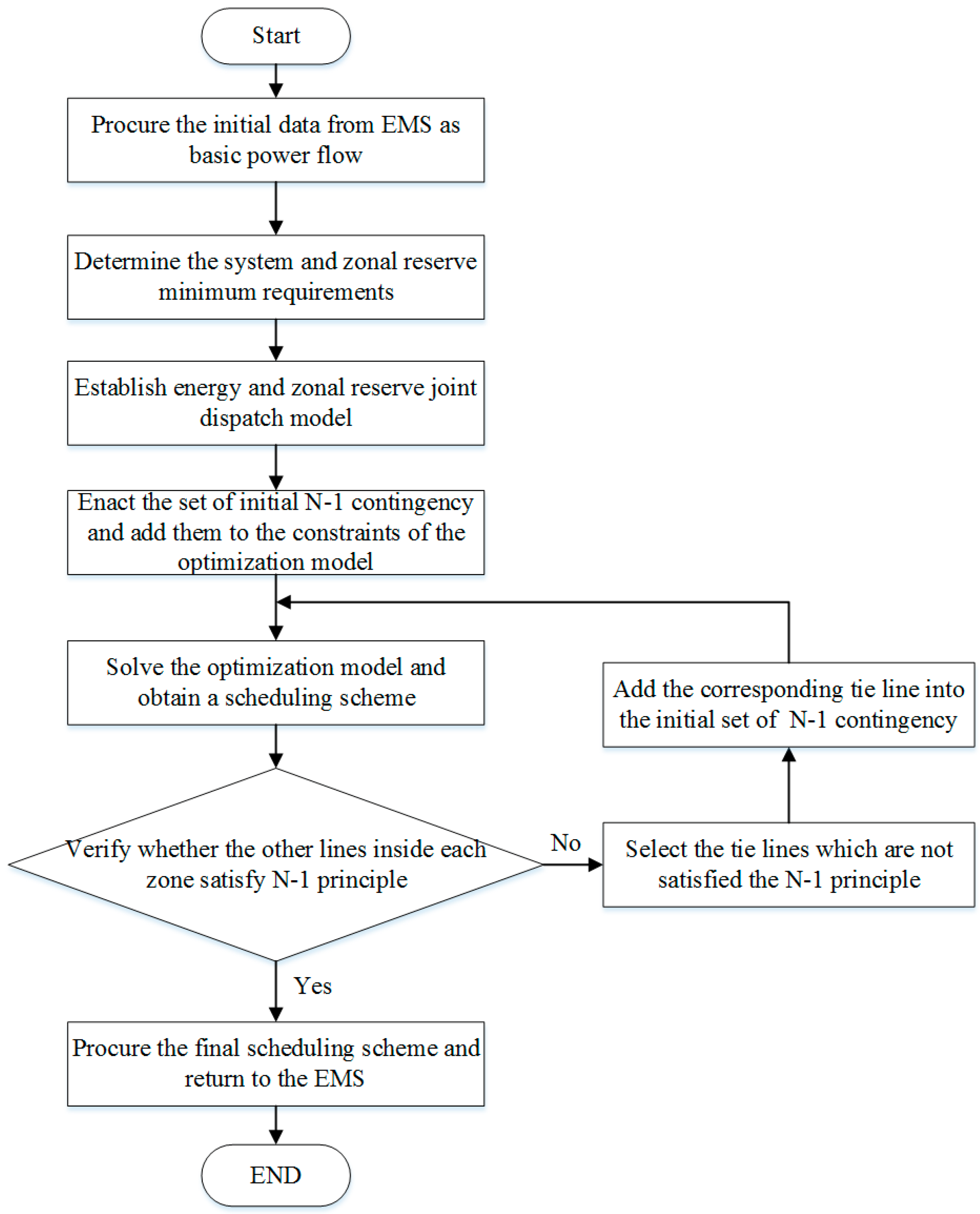
The N-1 security criterion of unit and transmission lines is executed to guarantee the feasibility of the initial scheduling scheme. Moreover, the utilization of the active set method can improve the efficiency of solution.

The rest of the paper is organized as follows: Section 2 presents the basic robust co-optimization model with energy and reserves to address the uncertainties from wind power generation. Section 3 employs the active set method to efficiently solve the co-optimization model in the consideration of N-1 contingencies for both generators and transmission lines. In Section 4, tests and comparisons under different scenarios are demonstrated. Finally, conclusions are drawn in Section 5.

2. Robust Co-Optimization to Energy and Reserve Joint Dispatch

The energy and reserve co-optimization dispatch model minimizes the total costs of energy and reserve, while obtaining an economically optimal dispatch schedule within the physical constraints. However, it is difficult to up-dispatch the reserve cleared by some generators due to the uneven distribution of generation resources in the entire system. Hence, a large-scale power system is divided into several geographic areas and the minimum system spinning reserve requirements and zonal spinning reserve requirements are considered at the same time to guarantee the deliverability of reserves when the contingency occurs. The feature of the proposed model is to incorporate minimum zonal requirements to guarantee the security and reliability of the power system. The objective function is then formulated as [5]

$$\min ({{\displaystyle \sum }}_{i=1}^{N_g}{e}_i{P}_i^{sch}+{{\displaystyle \sum }}_{a=1}^{N_a}{b}_a\left(A_a^{+}+A_a^{-}\right)+{{\displaystyle \sum }}_{i=1}^{N_g}{g}_i{R}_i)$$

(1)

where the three terms in the objective function represent the costs of energy, regulating reserve and spinning reserve, correspondingly. It should be noted that the coefficients (e_i, b_a, g_i) are the bidding price of energy, regulating reserve and spinning reserve of generators in the competitive deregulated power markets. The bidding prices are offered by the generation companies.

The constraints of the optimization model should include the power balance, generation output limits, ramp up/down limits, transmission line limits, system and zonal reserve requirements, such that

(a) Power Balance Constraint

$${{\displaystyle \sum }}_{i=1}^{N_g}{P}_i^{sch}={{\displaystyle \sum }}_{j=1}^{N_d}{D}_j$$

(2)

(b) Generation Output Limits

For AGC units, the energy and reserve generation should satisfy

$$P_a^{sch}+A_a^{+}+R_a\le P_{a\max }, P_a^{sch}-A_a^{-}\ge P_{a\min }$$

(3)

$$P_a^{sch}+A_a^{+}\le A_{a\max }, P_a^{sch}-A_a^{-}\ge A_{a\min }, a=1, \cdots ,N_a$$

(4)

For non-AGC units (dispatch-able units), the energy and spinning reserve generation should satisfy

$$P_i^{sch}+R_i\le P_{i\max },i=1,\cdots ,N_g$$

(5)

(c) The Limits of Up/Down Regulating Speed and Response Speed of Reserve

For two adjacent dispatch intervals, the ramp up and down rates should be limited by the constraints of dispatch-able units and AGC units respectively:

$$-T·r_i^{-}\le P_i^{sch}-P_{0i}\le T·r_i^{+}0\le R_i\le t_2·r_i^{+},i=1,\cdots ,N_g$$

(6)

$$0\le A_a^{+}\le t_1·r_a^{+}, 0\le A_a^{-}\le t_1·r_a^{-},a=1,\cdots ,N_a$$

(7)

(d) The System/Zonal Minimum Requirements for Reserves

Due to the uneven distribution of generation resources in actual power systems, the reserves may only locate in some specific zones if the reserve cost is very low in these regions and high in the others. This may result in difficulties in dispatching upwards the reserve cleared in some generators considering the limits of transmission line capacity and network congestion when a certain contingency really happens. In that case, there will be side effects on the security and reliability of the entire power system. Hence, it is essential to incorporate the zonal requirement constraints in the energy and reserve dispatch model.

Under normal circumstances, the system minimum requirement for regulating reserve and spinning reserve is

$${{\displaystyle \sum }}_{a=1}^{N_a}{A}_a^{+}\ge D_A^s, {{\displaystyle \sum }}_{i=1}^{N_g}{R}_i\ge D_R^s$$

(8)

The zonal minimum requirement for spinning reserve can be formulated as

$${{\displaystyle \sum }}_{i=1}^{N_g^z}{R}_i\ge D_R^z$$

(9)

where the given constant value $D_A^s$, $D_R^s$ and $D_R^z$ can be obtained by offline analysis and calculation.

(e) Limits of Transmission Line Capacity

$$-P_{l_k\max }\le P_{l_k}\le P_{l_k\max }, l_k\in {\Omega }_k$$

(10)

where $P_{l_k}$ can be obtained as

$$P_{l_k}={{\displaystyle \sum }}_{i=1}^{N_g}{H}_{ki}{P}_i^{sch}-{{\displaystyle \sum }}_{j=1}^{N_d}{H}_{kj}{D}_j+{{\displaystyle \sum }}_{m=1}^{N_w}{H}_{km}{W}_m^f$$

(11)

The above optimal dispatch model (1)–(11) is a deterministic optimization model, which dispatches the generation under the given forecasting wind power. However, the wind power generation is always stochastic. Therefore, the constraints in the above model (1)–(11) may be violated under the stochastic wind power output. To fully guarantee the operation constraints under the wind power output uncertainties, the regulating reserve provided by AGC units can response quickly to the mismatched power caused by fluctuations renewable energy outputs in the power system. In literature, the participation factor is utilized to determine the cleared regulating reserve in each AGC unit, as well as to formulate a robust scheduling scheme to the uncertainties of wind power generation outputs. Using the classical Equation (12), which assigns the outputs of regulating reserve to each AGC unit in the most economical way, the participation factors are fixed and formulated as [27].

$${\beta }_a=\frac{\raisebox{1ex}{$1$}\!\left/ \!\raisebox{-1ex}{$b_a$}\right.}{{{\displaystyle \sum }}_{a=1}^{N_a}\raisebox{1ex}{$1$}\!\left/ \!\raisebox{-1ex}{$b_a$}\right.}, a=1,2,\cdots ,N_a$$

(12)

To address the wind power uncertainties, the given forecasting error $E_m$ of each wind farm can be modeled as an interval $\left[E_m^{\min },E_m^{\max }\right],\mathrm{where} m=1,\cdots ,N_w$ and $m\in {\Omega }_w$. Specifically, $E_m$ is the forecasted error between the actual power output and the forecasted value of the wind farm m.

Then, according to Equation (A4) in the Appendix A, we will arrive at

$$-A_a^{-}\le {\beta }_a{{\displaystyle \sum }}_{m=1,m\in {\Omega }_w}^{N_w}{E}_m\le A_a^{+}, a=1,\cdots ,N_a$$

(13)

The constraint (13) represents the fact that the cleared regulating reserve $A_a^{+}$ and $A_a^{-}$ in each AGC unit should cover the assigned wind power uncertainties.

Considering the regulating reserve of generators with the participation of ${\beta }_a$ for re-dispatching the system from the basic scheduled generation outputs, the actual power flow of transmission lines can be written as Equation (14) according to the derivation in the Appendix A Equation (A5).

$$\begin{gathered} P_{l_k}={{\displaystyle \sum }}_{i=1,i\in {\Omega }_g}^{N_g}{H}_{ki}{P}_i^{sch}-{{\displaystyle \sum }}_{j=1,j\in {\Omega }_d}^{N_d}{H}_{kj}{D}_j+{{\displaystyle \sum }}_{m=1}^{N_w}{H}_{km}{W}_m^f \\ +{{\displaystyle \sum }}_{a=1}^{N_a}{{\displaystyle \sum }}_{m=1}^{N_w}\left(H_{ka}{\beta }_a+H_{km}\right)E_m \end{gathered}$$

(14)

However, re-dispatching the system may change the power flow and violations may occur. In order to guarantee that the system always stays within the security parameters, the constraint of transmission line should be modeled according to the derivation in Appendix A Equation (A11)–(A13):

$$\begin{gathered} {{\displaystyle \sum }}_{i=1,i\in {\Omega }_g}^{N_g}{H}_{ki}{P}_i^{sch}-{{\displaystyle \sum }}_{j=1,j\in {\Omega }_d}^{N_d}{H}_{kj}{D}_j+{{\displaystyle \sum }}_{m=1,m\in {\Omega }_w}^{N_w}{H}_{km}{W}_m^f \\ +{{\displaystyle \sum }}_{m=1,m\in {\Omega }_w}^{N_w}(y_{k,i}^{+}{E}_m^{\max }+y_{k,i}^{-}{E}_m^{\min })\le P_{l_k\max } \end{gathered}$$

(15)

$$\begin{gathered} {{\displaystyle \sum }}_{i=1,i\in {\Omega }_g}^{N_g}{H}_{ki}{P}_i^{sch}-{{\displaystyle \sum }}_{j=1,j\in {\Omega }_d}^{N_d}{H}_{kj}{D}_j+{{\displaystyle \sum }}_{m=1,m\in {\Omega }_w}^{N_w}{H}_{km}{W}_m^f \\ +{{\displaystyle \sum }}_{m=1,m\in {\Omega }_w}^{N_w}(y_{k,i}^{+}{E}_m^{\max }+y_{k,i}^{-}{E}_m^{\min })\ge -P_{l_k\max } \end{gathered}$$

(16)

with $y_{k,i}^{+}$ and $y_{k,i}^{-}$ being dummy matrices, which can be written as

$$\{\begin{array}{c}{y}_{k,i}^{+}\ge 0, y_{k,i}^{+}\ge {{\displaystyle \sum }}_{a=1,a\in {\Omega }_a}^{N_a}{H}_{ka}{\beta }_a+H_{ki} \\ y_{k,i}^{-}\le 0, y_{k,i}^{-}\le {{\displaystyle \sum }}_{a=1,a\in {\Omega }_a}^{N_a}{H}_{ka}{\beta }_a+H_{ki}\end{array}$$

(17)

3. Robust Co-Optimization Considering N-1 Constraints and Active Set Method

In this section, we will develop a robust energy and reserve joint dispatch co-optimization model considering N-1 contingency constraints for both transmission lines (or transformers) and generators, as well as the zonal reserve optimal placement and dispatch strategy. It is worthwhile to note that it is a “preventive” model, which is the supplemental of the initial model.

It is noted that the transmission lines and generators under the N-1 contingency have different impacts on the power system re-dispatch ability. Specifically, the N-1 contingencies on generators will result in the imbalance of active power while the shift distribution factor matrix is maintained. Consequently, the original dispatch scheme must be renewed and the reserve should be dispatched upwards to compensate the active power mismatch to deal with the contingency of the generator N-1. Thus, the optimal variables of the spinning reserve are to be reset and the model needs to be resolved so that the power balance is achieved (once the generator outage occurs). In contrast, the N-1 contingencies on transmission lines have no influence on the power balance constraint, but only the shift distribution factor matrix is changed. Since the power is still balanced (and thus the reserve and optimal variables remain), it only requires examining the limits for transmission line capacity under each contingency. Hence, the contingency constraints of transmission lines and generators are treated separately as follows:

3.1. N-1 Contingency Constraints for Transmission Lines

Assuming that the s-th transmission line in the pre-defined set is out of service, the topology of grid will be changed. Consequently, the generation shift distribution factor ${\mathit{H}}^s$ must be renewed and recalculated. It should be noted that transformers can be modeled as transmission lines in the optimization model, and here the transformers are taken as transmission lines in N-1 contingencies. Therefore, the transmission lines under N-1 contingency are subjected to:

$$-P_{l_k\max }\le P_{l_k}^s\le P_{l_k\max }$$

(18)

$$\begin{gathered} P_{l_k}^s={{\displaystyle \sum }}_{i=1,i\in {\Omega }_g}^{N_g}{H}_{ki}^s{P}_i-{{\displaystyle \sum }}_{j=1,j\in {\Omega }_d}^{N_d}{H}_{kj}^s{D}_j+{{\displaystyle \sum }}_{m=1,m\in {\Omega }_w}^{N_w}{H}_{km}^s{W}_m^f \\ +{{\displaystyle \sum }}_{a=1,a\in {\Omega }_a}^{N_a}{{\displaystyle \sum }}_{m=1,m\in {\Omega }_w}^{N_w}\left(H_{ka}^s{\beta }_a+H_{km}^s\right)E_m \end{gathered}$$

(19)

where $P_{l_k}^s$ is the active power flow of the transmission line k when the pre-defined transmission line s is broken and $H_{ki}^s$ is the element located in (k, i) in the renewed shift distribution factor matrix ${\mathit{H}}^s$.

3.2. N-1 Contingency Constraints for Generators

Once a failure occurs on the pre-defined n-th generator, its output as well as the regulating reserve and spinning reserve will be forced to zero. It leads to

$$P_n=0,A_n^{+}=0,A_n^{-}=0,R_n=0$$

(20)

Meanwhile, the requirements of the minimum system regulating and spinning reserve must be satisfied, and it yields

$${{\displaystyle \sum }}_{a=1,a\ne n}^{N_g}{A}_a^{+}\ge D_A$$

(21)

$${{\displaystyle \sum }}_{a=1,a\ne n}^{N_g}{A}_a^{-}\ge D_A$$

(22)

$${{\displaystyle \sum }}_{i=1,i\ne n}^{N_g}{R}_i\ge D_R$$

(23)

If one contingency occurs on the n-th generator, the cleared spinning reserves of the other normal online generators should be dispatched upwards and the active power output should be increased to compensate the power mismatch.

$${{\displaystyle \sum }}_{i=1,i\ne n}^{N_g}{R}_i^n=P_n$$

(24)

where $R_i^n$ represents the spinning reserve that the i-th generator should actually use to re-dispatch the power generation after the n-th pre-defined generator outage occurs. However, the reserve should not be larger than the cleared spinning reserve of the i-th generator.

$$0\le R_i^n\le R_i$$

(25)

After dispatching the spinning reserve upwards, the constraints of transmission lines must still be satisfied:

$$-P_{l_k\max }\le P_{l_k}^n\le P_{l_k\max }$$

(26)

$$\begin{gathered} P_{l_k}^n={{\displaystyle \sum }}_{i=1,i\in {\Omega }_g}^{N_g}{H}_{ki}\left(P_i+R_i^n\right)-{{\displaystyle \sum }}_{j=1,j\in {\Omega }_d}^{N_d}{H}_{kj}{D}_j+{{\displaystyle \sum }}_{m=1,m\in {\Omega }_w}^{N_w}{H}_{km}{W}_m^f \\ + {{\displaystyle \sum }}_{a=1,a\in {\Omega }_a}^{N_a}{{\displaystyle \sum }}_{m=1,m\in {\Omega }_w}^{N_w}\left(H_{ka}{\beta }_a+H_{km}\right)E_m \end{gathered}$$

(27)

where $P_{l_k}^n$ represents the power flow in the k-th transmission line in the grid after the outage of the n-th pre-defined generator.

Furthermore, the contingency constraints of both transmission lines and generators are added into the joint robust co-optimization model. However, if all the N-1 contingencies of the generators and transmission lines are added into the optimization model, there will be a large number of variables and constraints in the model and the computational speed will be significantly affected in real-time electricity market. To improve the computational performance, an active set method is employed to add only some vital N-1 contingencies of generators and transmission lines into the model; the other constraints are simply checked any other violated constraints are added into the model. The renewed co-optimization model is then solved and the new dispatch schedule is obtained. Then, a recursive process is conducted until all the constraints are satisfied, which can be found in Figure 1.

(a)

The participation factors are introduced to determine the regulating reserve cleared in the AGC units to balance the predicted errors of wind power generation outputs;

(b)

Through a great deal of power system stability and reliability offline simulation analysis, together with the forecasted wind generation outputs, the market wide requirement and each zonal requirement for regulating reserves and spinning reserves are determined;

(c)

Along with the basic constraints of the traditional economic dispatch model, the energy and zonal reserve joint dispatch model, considering wind power generation uncertainties to minimize the total energy and reserve costs, is established. In addition, the market wide requirement and each zonal requirement for reserves are taken into account in the constraints;

(d)

In the optimization model, contingencies on both generators and transmission lines are modeled explicitly. Since the N-1 contingencies on transmission lines and generators have different impacts on the re-distribution of the power flow, the modeling of the two elements is done separately.

(e)

To alleviate the computational burden, the contingency constraints are added into the model sequentially, and then all of contingencies will be examined whether all the N-1 feasibility criteria are satisfied. If one contingency check is failed, the N-1 constraints corresponding to this line outage will be added into the active set and further incorporated into the constraints of the above optimization model in Step 4. The new optimization model will be formulated and solved to obtain a new dispatch schedule. Repeat the above N-1 feasibility criteria check until all the N-1 contingency constraints are satisfied to formulate a feasible dispatch schedule in actual real-time electricity market.

4. Numerical Results

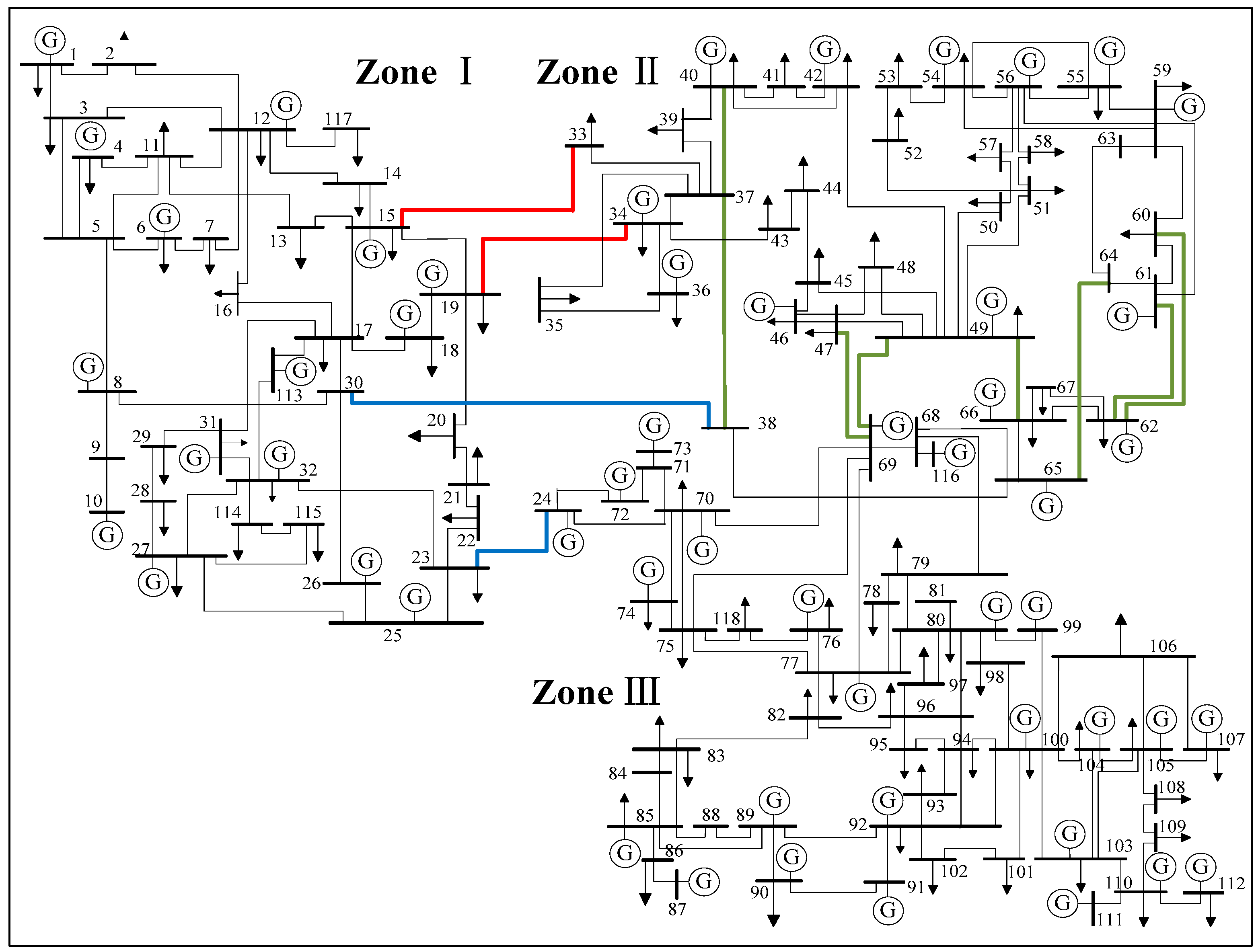
In this section, the IEEE-118 bus test system with 6 wind farms is formulated, including 91 load buses, 54 generators and 186 transmission lines. The information of each generator and the information of load demand are available from MATPOWER 5.1 [28]. The entire system is geographically divided into three zones as shown in Figure 2. There are nine AGC units in the system assigned to three zones, respectively. The AGC units at bus #6, #12 and #15 are assigned to Zone I; those at bus #34, #36 and #40 are assigned to Zone II; and the units at bus #70, #72 and #73 are assigned to Zone III. The 11 zonal interconnection lines are highlighted in Figure 2. The regulating reserve system requirement is determined by offline study and denoted as $D_A^s$ and $D_R^s$, as shown in

Table 1. System/zonal regulating and spinning reserve minimum requirements (MW). Regulating reserve system requirement$({\mathit{D}}_{\mathit{A}}^{\mathit{s}})$; system spinning reserve minimum requirement (${\mathit{D}}_{\mathit{R}\mathbf{1}}^{\mathit{s}})$; maximum installed capacity among all the generators $({\mathit{D}}_{\mathit{R}\mathbf{2}}^{\mathit{s}})$.

Minimum Requirements of Regulating and Spinning Reserve			Minimum Requirements of Zonal Regulating and Spinning Reserve
${\mathit{D}}_{\mathit{A}}^{\mathit{s}}$	${\mathit{D}}_{\mathit{R}1}^{\mathit{s}}$	${\mathit{D}}_{\mathit{R}2}^{\mathit{s}}$	Zone I	Zone II	Zone III
42.42	339.36	805.2	96.3	134.2	193.7

. It is assumed that the wind farms are installed at bus #4, #8, #18, #44, #66 and #69. The basic predicted output value is denoted as vector $\mathit{w}=\left[80;100;120;160;120;140\right]$ MW and the ratio of the predicted error to the basic predicted output value is denoted as the uncertainty degree α, which reflects the level of wind power generation uncertainty. A large α implies that the wind power output has large uncertainty. In addition, the proposed method is performed using MATLAB2015a, CPLEX 12.5 and MATPOWER on a personal computer with Intel^®Core^TM i7 Processor 6500U (2.5 GHz) and 4 GB RAM.

Note that the purpose of the deployment of the regulating reserve in this paper is to balance the forecasted error of wind power generation outputs; we hereby assume that the forecasted load data is relatively accurate. As explained in [29], the requirement of the reserve can be determined by a certain ratio of the load demand. According to the empirical data and off-line calculation results from MISO [17], the system regulating reserve minimum requirement is assumed as 1% of the basic total load plus wind power uncertainties. Moreover, the system spinning reserve minimum requirement is assumed as 8% of the total load (denoted as $D_{R1}^s$). At the same time, the system spinning reserve minimum requirement should be above the maximum installed capacity among all the generators (denoted as $D_{R2}^s$). The zonal spinning reserve minimum requirement is procured by the practical power system operation experience and offline simulation results. In addition, considering that after N-1 contingency occurs, transmission line congestion may lead to the cleared reserve being unable to deploy, the zonal spinning reserve minimum requirement is assumed to be 10% of this zonal load demand. The concrete calculation results are listed in Table 1.

Furthermore, the analysis on the feasibility and economy of solved solutions from the proposed optimization model is studied in Figure 3 and

Table 2. Regulating reserve cost under different wind generation uncertainty scenarios and load levels.

Uncertainty Degree	Load Level	1.00	1.05	1.10	1.15	1.20	1.25
0%	Costs (YUAN)	10,491	11,053	11,631	12,310	13,156	13,733
10%	Costs (YUAN)	20,810	21,822	22,834	23,846	24,858	25,870
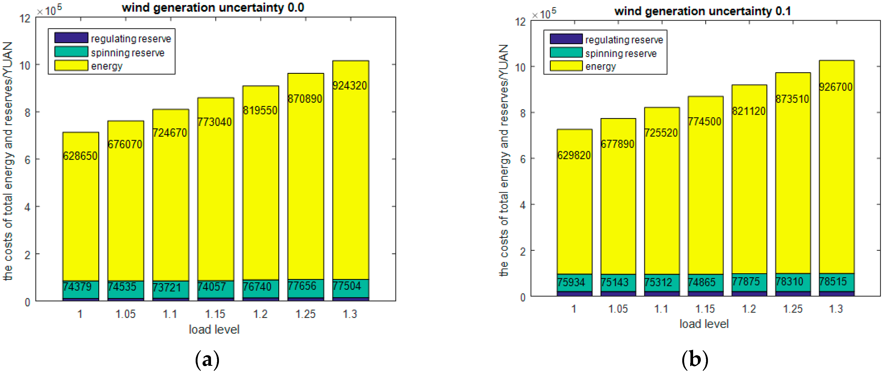
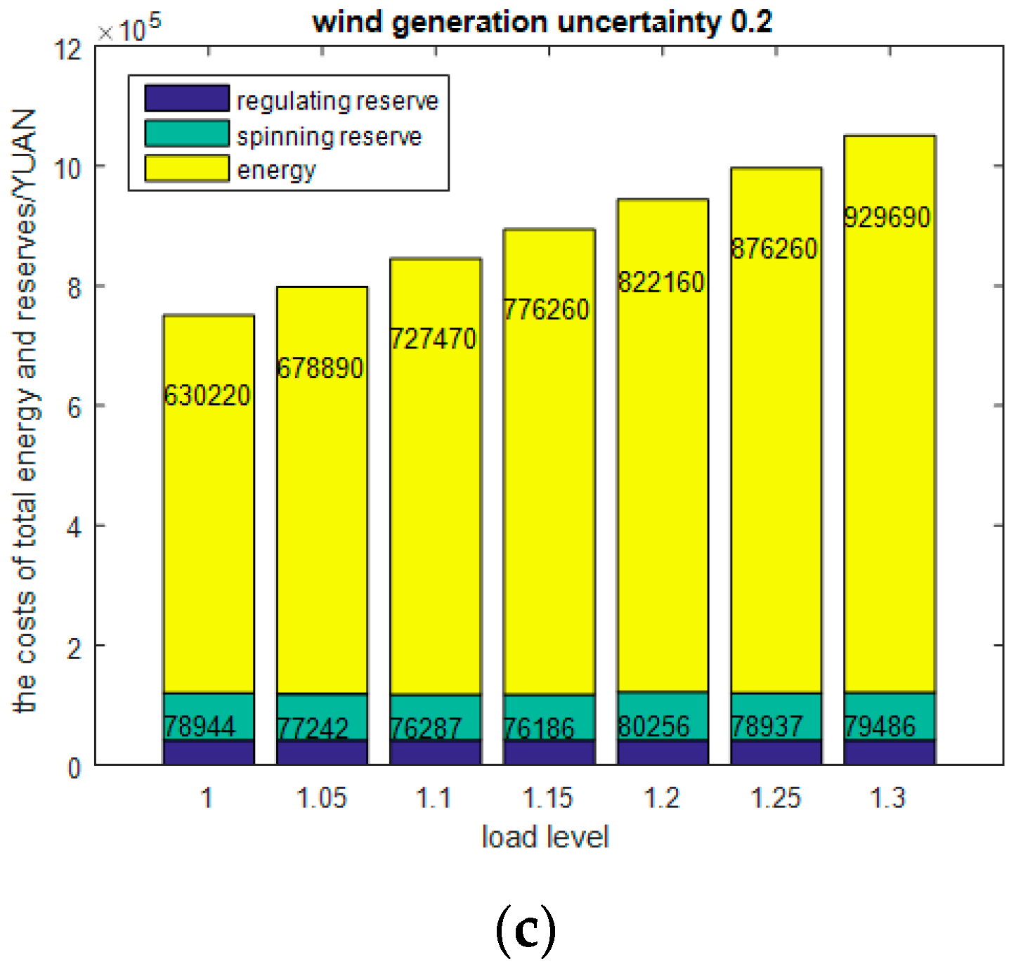
20%	Costs (YUAN)	41,620	43,761	45,902	48,043	50,184	52,325

. By setting different parameters of load levels (1.0, 1.05, 1.10, 1.15, 1.20 and 1.25 times of the rated load under normal condition) and wind power uncertainty degrees (0.0, 0.1 and 0.2), the proposed optimization model can be solved accordingly by the CPLEX optimizers (IBM, New York, NY, United States).

Table 2 shows the optimal regulating cost under different wind generation uncertainty scenarios and load levels, which suggests that for a given uncertainty degree of the wind power generation, the regulating reserve cost will increase slightly due to the slightly increase in the load level. In contrast, for a given load level, the regulating reserve cost will increase significantly with the increase of uncertainty degree, due to the large increase in the uncertainty degree of the wind power generation. This implies that the large uncertainty degree requires more regulating reserve to guarantee the power balance, which is represented by the Equations (13), (21) and (22). Therefore, the regulating reserve cost will increase.

More concretely, Figure 3 depicts the optimal energy and reserve costs under different load levels and wind power uncertainty degrees. The energy cost for any given load level increases along with the wind power uncertainty degree. This is because more regulating reserve is needed to cope with the wind power uncertainties, which will further sacrifice the generation cost to ensure a robust solution. Since both the reserve cost and energy cost will increase with the increase of load levels and uncertainty degrees, the total cost will increase as well. Moreover, the results in Table 2 and Figure 3 also illustrate that the regulating reserve cost will increase significantly with the increasing uncertainty of wind power generation output, while the energy cost will increase significantly with the increasing load level. Meanwhile, Table 2 and Figure 3 also suggest the mutual growth of energy and reserve costs when the uncertainties of wind power generation output and load level are increasing. Based on the analysis on the feasibility and economy, it is notable that the simulation results can provide the theoretical and experimental knowledge for the operators in the practical operation of the power system with large-scale wind power generation.

Meanwhile,

Table 3. Spinning reserves in each zone with/without consideration of zonal reserve.

	Wind Power Uncertainty	0	0.05	0.10	0.15	0.20	0.25	0.30
Spinning Reserve
With consideration of zonal reserve (MW)	I	358.58	360.35	349.70	339.06	328.41	317.76	307.11
	II	134.20	134.20	134.20	134.20	134.20	134.20	134.20
	III	312.42	310.65	321.30	331.94	324.59	353.24	363.89
Without consideration of zonal reserve (MW)	I	420.00	420.00	420.00	420.00	420.00	415.03	397.00
	II	0.00	7.39	14.77	22.16	29.54	36.93	44.32
	III	385.20	377.81	370.43	363.00	355.65	353.24	363.89

compares the spinning reserves in each zone with/without consideration of the zonal reserve placement, and the results suggest that the dispatch model obtains a better distributed result of the spinning reserve in each generator in the consideration of the zonal reserve placement. In particular, without considering the zonal reserve placement, some zones may have few spinning reserves cleared in generator, which is far below the minimum requirements of the zonal reserve from offline analysis. This will significantly affect the reliability of the system under the N-1 contingency in the zone, where the transmission bottlenecks inhibit the deliverability of the reserve.

Finally, the computational time of four different solution strategies to deal with N-1 transmission line contingencies in the co-optimization model is shown in

Table 4. Computational time of four treatments of N-1 line contingency (s) and the transmission line number (which are violated N-1 contingency constraints in “C-L” robust joint dispatch). The robust joint dispatch modeling N-1 contingencies of all transmission lines simultaneously in the optimization model (A-L); the robust joint dispatch without the consideration of N-1 contingency constraints of transmission lines and generators (N-L); the robust joint dispatch only taking the vital N-1 contingency constraints for transmission lines into account (C-L); the active set method to sequentially add the N-1 contingency constraints into the model and solve the model iteratively (I-L).

Methods	N-L	C-L	I-L	A-L
Time (s)	0.1716	0.8418	3.2926	43.3617
Violated Transmission Lines	#44, #51, #54, #76, #79, #84, #88, #90,#105, #106	#76, #79, #84, #88, #90	-	-

. As shown in the above model, the security/contingency constrained approach is based on the DC (direct current) power flow, and the computational tractability has been guaranteed by introducing the Equations (15)–(17). Therefore, all the constraints and the objective function of the model are linear, resulting in a very efficient computational behavior.

“A-L” represents the robust joint dispatch modeling N-1 contingencies of all transmission lines simultaneously in the optimization model. “N-L” is the robust joint dispatch without the consideration of N-1 contingency constraints of transmission lines and generators. “C-L” is the robust joint dispatch only taking the vital N-1 contingency constraints for transmission lines into account. “I-L” refers to the active set method to sequentially add the N-1 contingency constraints into the model and solve the model iteratively.

Obviously, the A-L method, taking into account all the transmission lines in the robust optimization model, can fully address the security of transmission lines without any violation, but it requires more computational burden and challenges the real-time electricity markets, especially for large-scale power systems.

Although N-L needs about 0.1716 s, which is much slower than other three strategies, this method cannot guarantee the transmission security. For instance, the transmission lines {#44, #51, #54, #76, #79, #84, #88, #90, #105, and #106} will violate the transmission line limit. Meanwhile, C-L method only considers vital N-1 contingency constraints, which need 0.8418s. However, this method still cannot fully guarantee the feasibility in real-time power markets, transmission lines {#76, #79, #84, #88, #90} can still be violated under other contingencies. When employing the active set method to formulate the N-1 contingency constraints and solving the model iteratively, the computational time is about 3.2926 s. Compared to the C-L robust joint dispatch, the proposed I-L method sacrifices only little time but the transmission security can be fully guaranteed as the A-L method. Moreover, compared to the A-L method considering all the N-1 contingencies of transmission lines, the computational time using the iterative solution can be significantly improved while leading to the same solution.

5. Conclusions

In this paper, a robust co-optimization to energy and zonal reserve joint dispatch model has been proposed to address the uncertain wind power generation in real-time electricity markets. Specifically, the regulating reserve is utilized to balance the forecast errors of the uncertain wind generation, and the spanning reserve is employed in the case of the power system contingencies. Moreover, the model geographically divides the entire power system into several parts and sets the minimum requirements for each zone to guarantee that the reserve can be effectively dispatched upwards under the contingency. Finally, an active set method has been employed to solve the proposed model. Numerical results on the IEEE 118-bus system have demonstrated the feasibility of the proposed robust co-optimization model. With the increase of the load level and uncertainty of wind generation output, the total costs will increase accordingly. Moreover, the comparison between proposed active set method and the other methods show that the proposed method can fully guarantee the system security, while achieving a better computational efficiency. This good performance can have potential applications in the real-time electricity market.