Developing Computational Fluid Dynamics (CFD) Models to Evaluate Available Energy in Exhaust Systems of Diesel Light-Duty Vehicles

Abstract

Around a third of the energy input in an automotive engine is wasted through the exhaust system. Since numerous technologies to harvest energy from exhaust gases are accessible, it is of great interest to find time- and cost-efficient methods to evaluate available thermal energy under different engine conditions. Computational fluid dynamics (CFD) is becoming a very valuable tool for numerical predictions of exhaust flows. In this work, a methodology to build a simple three-dimensional (3D) model of the exhaust system of automotive internal combustion engines (ICE) was developed. Experimental data of exhaust gas in the most used part of the engine map in passenger diesel vehicles were employed as input for calculations. Sensitivity analyses of different numeric schemes have been conducted in order to attain accurate results. The model built allows for obtaining details on temperature and pressure fields along the exhaust system, and for complementing the experimental results for a better understanding of the flow phenomena and heat transfer through the system for further energy recovery devices.

1. Introduction

Around a third of the fuel energy in a light-duty diesel engine is wasted through the exhaust system [1]. Rising awareness of environmental issues together with the fuel economy have encouraged research on energy recovery [1,2] from exhaust gas. An obvious first step for energy recovery is evaluating the heat source. The nature of exhaust flow changes during engine operation. Hence, there is a need for models that allow evaluating exhaust gas in a cost- and time-efficient manner under different engine conditions.

Computational fluid dynamics (CFD) is becoming a very popular tool for numerical predictions in the automotive industry. CFD models are employed in five major areas: vehicle aerodynamics, thermal management (cooling and climate control), cylinder combustion, engine lubrication and exhaust system performance. The main applications of CFD in exhaust systems are: flow distribution in the front of the monolith, pressure loss through exhaust system, skin temperature prediction, heat loss analyses and emission-related studies [3].

High levels of energy lost through engine exhaust have brought attention to heat transfer in exhaust systems and how to model associated phenomena.

In Konstantinidis et al. [4], the status of knowledge regarding heat transfer phenomena in automotive exhaust systems was summarized, and a transient model covering diverse exhaust piping configurations was presented. Using this model, Kandylas et al. [5] studied heat transfer in automotive exhaust pipes for steady and transient conditions. It is stated that the code is suitable to support a complete and efficient methodology for design optimization.

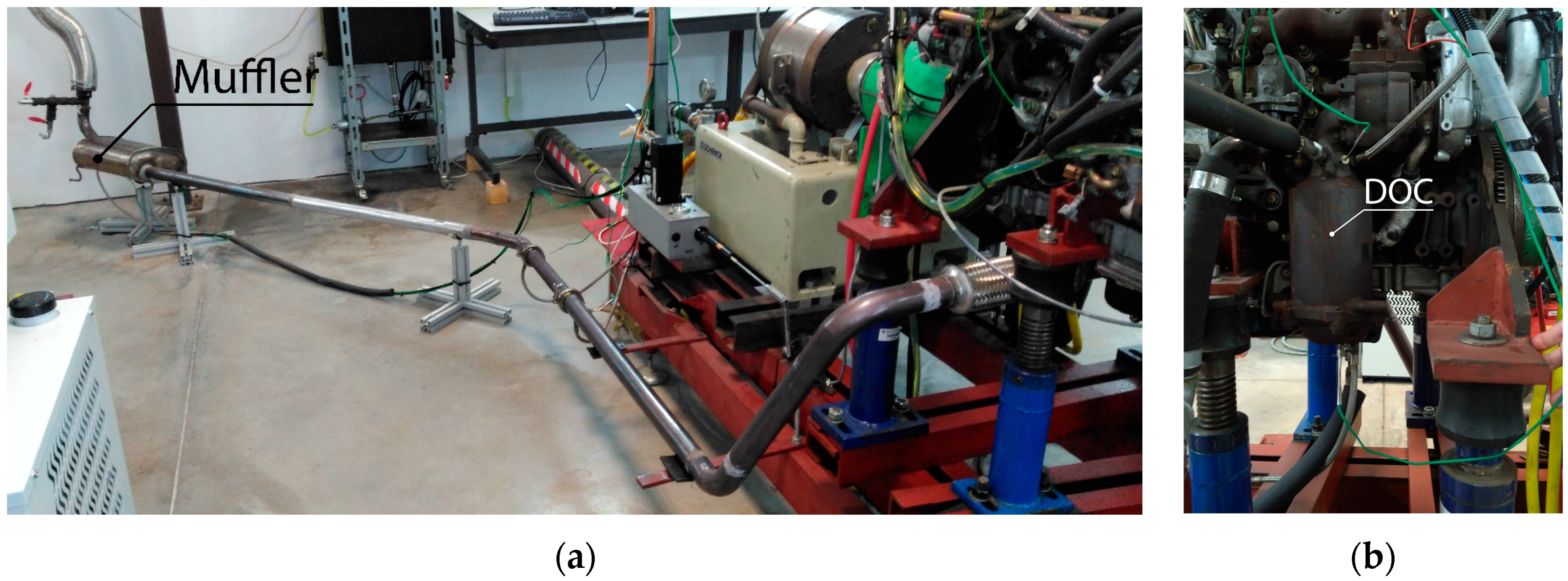
Not only are exhaust heat transfer and temperature models important for energy recovery, but also for on-board control and diagnosis of the after-treatment system. In the work of Guardiola et al. [6], diesel oxidation catalyst (DOC) inlet temperature was modelled depending on fuel mass flow and engine speed using an engine map look-up table.

Traditionally, one-dimensional (1D) simulations using in-house or commercial codes have been used to study exhaust flow. In Shayler et al. [7], a 1D model of system thermal behavior was developed. The exhaust system is modelled as connected pipe and junction elements with lumped thermal capacities. Heat transfer correlations for quasi-steady and transient conditions were investigated. The computational model supports studies of exhaust and after-treatment system design, the investigation of thermal conditions, and performance characteristics. Model predictions and experimental data were in good agreement.

In Kapparos et al. [8], a 1D heat transfer model in an automotive diesel exhaust is presented. The external natural convective heat transfer coefficient was given by Churchill and Chu’s correlation. A sensitivity analysis of the main variables (heat transfer coefficient, external pipe emissivity and others) affecting heat transfer in exhaust pipes was carried out. Fu et al. [9] developed a 1D model of an exhaust pipe (without the catalytic converter). Apart from typical variables studied, effects of pipe geometry and flow regime were investigated.

One-dimensional tools have the advantage of shorter computational time, but the accuracy of the results is limited by their inability to simulate 3D flow effects in regions such as the inlet and outlet cone. Usually strong turbulent flow exists when angled and asymmetrical cones are presented [3].

Three different approaches were used in Fortunato et al. [10] to simulate the exhaust and underbody of the car: 1D, 3D finite elements and 3D complete thermo-fluid-dynamics. Both 3D models allowed to detect the most critical points in terms of higher temperatures

In Chuchnowski et al. [11], temperature distribution and heat flow analyses on the exhaust system of a mining diesel engine to determine technical parameters of a heat recuperation system are presented. Three-dimensional numerical simulations show it is possible to develop a suitable design of an energy recovery device.

Simulations in a coupled three-dimensional thermal model including the underhood, underbody and exhaust systems of a vehicle were conducted by Guoquan et al. [12]. Pulsating flow and steady flow effects were compared. Pulsating exhaust showed an enhancement of more than a 10% in heat transfer. Influence of this effect was higher at the final components of the exhaust, such as the muffler.

Research has also been focused on finding optimal position for exhaust components. Durat et al. [13] compared experimental and CFD heat transfer results in an exhaust system of a spark-ignition engine. An optimal position of a close-coupled catalytic converter in terms of light-off time was found using the CFD model. Liu [14] developed a 3D exhaust model to study the optimal position of a heat recovery device. Three different simulations were carried out varying the position of a thermoelectric generator along the system. Higher surface temperature and lower backpressure were obtained when the recovery device was placed between catalytic converter and muffler. The influence of materials and insulation on heat transfer in catalytic converters has also been discussed employing a 3D model [15].

In the same way preceding authors have employed CFD simulations successfully to find an optimal position for exhaust components or to assist in their design, CFD can also be used to gain knowledge of the relevant characteristics of the flow in terms of its usage in energy recovery. Previous works [16] state that knowledge of heat transfer within the gas is critical to enhance harvested energy.

In exhaust systems, not only should heat transfer to surroundings be reproduced but also chemical reactions in catalytic processes, since after-treatment devices can modify gas temperature. Most mathematical kinetics models rely on the Langmuir-Hinshelwood expressions derived on pellet-type Pt catalysts for the CO and HC oxidation with modified parameters (activation energies and activity factors), best suited to the case modeled. This approach is widely employed because it provides acceptable accuracy in the most common automobile range of operation.

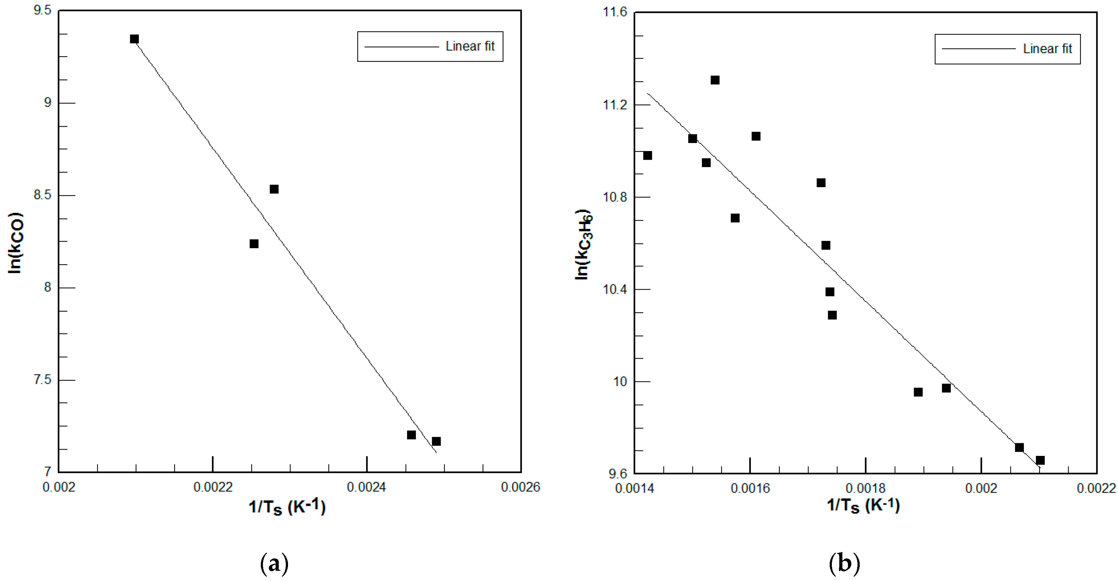
Measurements on pellet-type platinum-alumina catalysts have been processed [17] to derive kinetic rate expressions for the oxidation reactions of CO and C₃H₆ under oxygen-rich conditions for a better understanding of platinum oxidation catalysts in automotive emission control systems. Terms accounting for CO, C₃H₆ and NO inhibition were included. The isothermal reactor approach in a numerical integration-optimization method was used to fit the kinetic parameters. These expressions, especially as written by Oh et al. [18], have been widely used [19,20,21,22]. This approach has also been used to build simpler kinetic models over a range of interest [23].

Detailed kinetics for a Pt/Rh three-way catalyst were described in Chatterjee et al. [24]. The model consists of 60 elementary reaction steps and one global reaction step, involving 8 gas species and 23 site species. It considers the steps of adsorption of the reactants on the surface, reaction of the adsorbed species, and desorption of the reaction products. This approach includes a mechanism of C₃H₆ oxidation on Pt/Al₂O₃, a mechanism of NO reduction on Pt, and a mechanism for NO reduction and CO oxidation on Rh. This model has been used when more accuracy is required, as in Kumar et al. [25].

Nevertheless, due to the variety of washcoat materials and loadings of the monoliths and to ageing effects of after-treatment devices, the kinetic parameters published have difficulties in fitting to conditions or catalytic converters different from the study cases. To overcome the difficulty of finding kinetic parameters fitted to their application, it would be of interest to have a simple method for researchers to develop their own kinetic constants for CFD exhaust models.

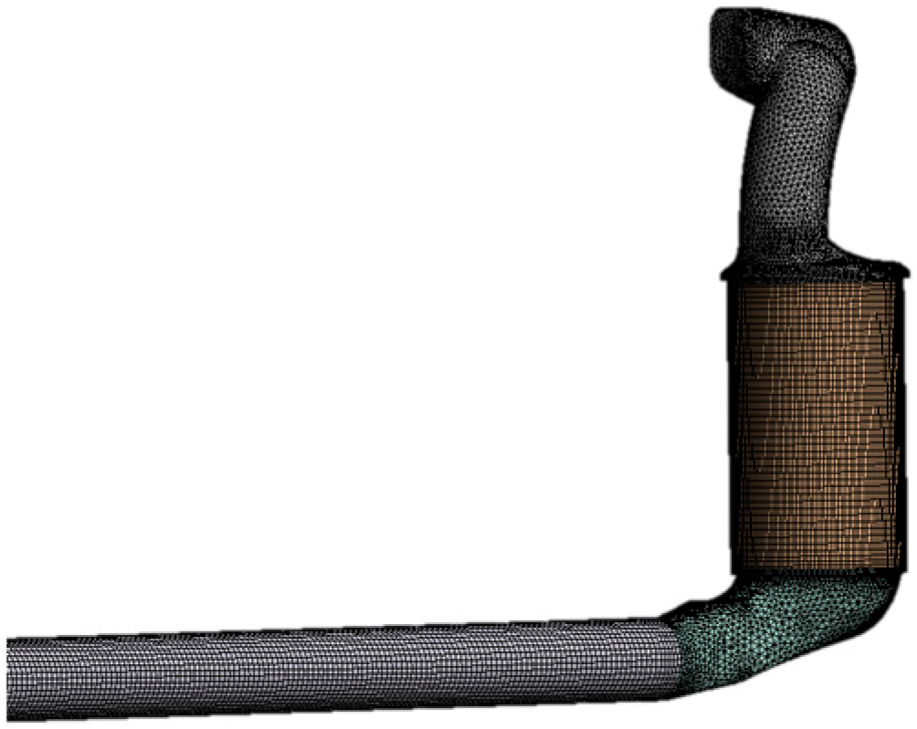
The real physical space of a full-size monolith converter contains thousands of tiny channels and could present an extremely time-consuming problem to solve. There are several approaches to modeling the monolith of a catalytic converter. For simulations of the converter performance, most models use a volume-averaging method and treat the monolith as a continuous porous medium [23,24,25,26]. With the porous medium, approach channels are not simulated but a macroscopic understanding of the flow is achieved while keeping the computational requirements affordable.

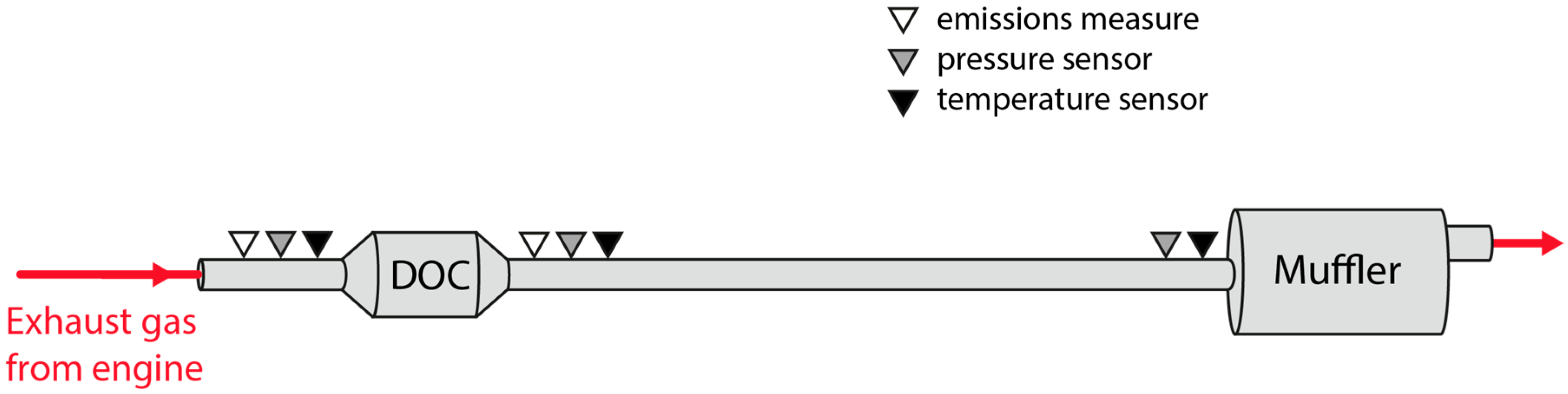
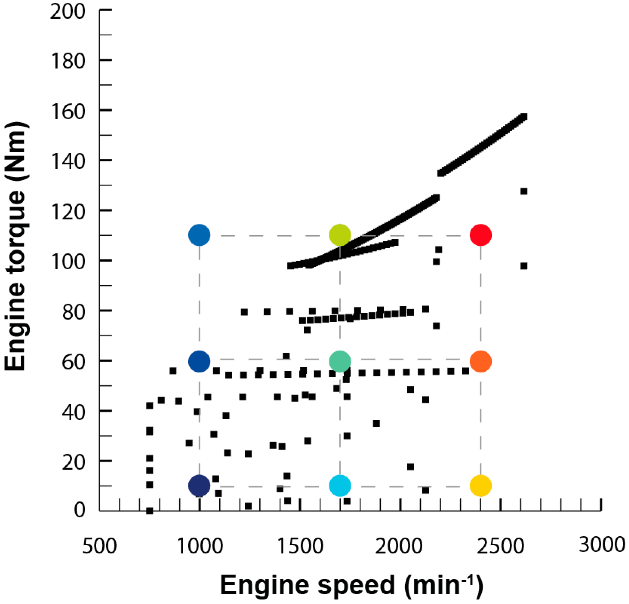
The scope of this work is to develop a combined theoretical and experimental methodology to build an exhaust model to obtain information about temperature and heat losses along the system. Results were used to provide an insight into those flow characteristics that must be taken into account when harvesting energy, especially but not exclusively for thermoelectric modules. The model does not only intend to reproduce the behavior of the exhaust system at a single operation point but in the whole most-used part of the engine map. This information is needed to evaluate the exhaust gas energy available for recovery under real operating conditions.

2. Materials and Methods

2.1. Materials

2.1.1. Engine

Tests were carried out in a test-bench with a Nissan YD22 four-stroke, turbocharged, four-cylinder diesel engine. The engine bore and stroke are, respectively, 86 mm and 130 mm, and the compression ratio is 16.7:1. The exhaust system (Figure 1) is equipped with a diesel oxidation catalyst (DOC) and a muffler.

2.1.2. Measurement Devices

Piezo resistive pressure sensors and K-type thermocouples were used for measuring pressure and temperature of the gas along the exhaust system (see Figure 2). The exhaust mass flow rate was calculated from the addition of fuel and air mass flow rates. Skin temperatures used in calculations were provided by the IR camera Gobi-384 GigE.

Pollutants are measured using an ENVIRONNEMENT manufacturer equipment. A TOPAZE 32M model was used as NO_x analyser, based on the chemiluminescence effect from NO oxidation by ozone (O₃). The GRAPHITE 52M gas analyser measures total hydrocarbons (THCs) by flame ionization detection while a MIR 2R gas analyser measures CO and CO₂ species, detecting the molecules absorption in the infrared spectrum. Other species compositions are estimated via chemical balances from fuel and air consumption.

2.2. Methods

2.2.1. Test Plan

The velocity profile imposed by the New European Driving Cycle (NEDC) used for light-duty vehicle certification was translated into engine operating conditions (torque and engine speed), as shown in Figure 3 (black squares), employing longitudinal dynamics equations [27,28]. Then, a matrix of nine steady-state modes (see Figure 3, circles) covering the most-used quarter of the engine map under both urban and extra-urban NEDC conditions was selected for testing.

2.2.2. Experimental Characterization of Model Input Parameters

(a) Monolith pressure loss characterization.

The classical approach that links pressure drop and velocity in flows through porous media is the Forchheimer equation (Equation (1)), that can be derived from the Navier–Stokes equation for one-dimensional, incompressible and steady laminar flow of a Newtonian fluid in a rigid porous medium [29]:

$$-\frac{dp}{dx}=\frac{1}{\kappa }\left(\mu ·v\right)+\beta \left(\rho ·v^2\right)$$

(1)

The second term in the right can be interpreted as a second-order correction to account for the contribution of inertial forces, but, at sufficiently low velocities, this effect is negligible and Equation (1) can be reduced to Darcy’s law (Equation (2)) [30]:

$$-\frac{dp}{dx}=\frac{1}{\kappa }\left(\mu ·v\right)$$

(2)

Darcy’s law can be rewritten in the form of Equation (3), relating the average fluid velocity $v$ through the pores with pressure drop $\Delta p$ along a segment of length $L$.

$$-\frac{\Delta p}{\mu L}=\frac{1}{\kappa } v$$

(3)

If the equation from the linear fit of the scatter plot of $-\frac{\Delta p}{\mu L}$ vs. $v$ is (Equation (4)):

$$Y=BX$$

(4)

then Darcy’s constant $\kappa$ can be derived as follows (Equation (5)):

$$\kappa =\frac{1}{B}$$

(5)

(b) Heat transfer to surroundings.

Natural convection to pipe surroundings in the test-bench needs to be included. Wall temperatures along the exhaust pipe were measured using thermography. Figure 4 shows, as an example, views of the external surface of the pipe and the DOC.

An average skin temperature was used to calculate an effective convection heat transfer coefficient. This skin temperature simplification is considered as reasonable, since calculation of heat transfer rates is not very sensitive in the values of pipe wall temperatures [5].

Total transferred heat from pipe wall to surroundings is $\dot{Q}$ (W) (Equation (6)):

$$\dot{Q}={\overline{h}}_{\infty }\pi d\left(T_{wall}-T_{\infty }\right)+\epsilon \pi dL\sigma \left(T_{wall}^4-T_{amb}^4\right)$$

(6)

Here, all terms in the right side of Equation (6) are grouped in one single equivalent convection term (Equation (7)):

$$\dot{Q}={\overline{h}}_{eff}\pi dL\left(T_{wall}-T_{\infty }\right)$$

(7)

The effective convection coefficient accounts for convection and radiation heat losses, although radiation heat transfer to the environment is expected to be low, since wall temperature is below 400 °C [4]. A similar approach is explained in Kapparos et al. [8].

Based on the measured exhaust gas and pipe wall temperatures, an energy balance for the exhaust gas is employed for the calculation of the heat flux. The resulting heat fluxes are employed in the estimation of a mean gas-to-wall convection coefficient.

Since temperature at both ends of the exhaust pipe are measured, total heat losses $\dot{Q}$ (W) can be obtained as Equation (8):

$$\dot{Q}={\dot{m}}_g{c}_p{,}_g\left(T_{g,in}-T_{g, out}\right)$$

(8)

Equaling Equations (7) and (8), ${\overline{h}}_{eff}$ can be derived as Equation (9):

$${\overline{h}}_{eff}=\frac{{\dot{m}}_g{c}_p{,}_g\left(T_{g,in}-T_{g, out}\right)}{\pi d\left(T_{wall}-T_{\infty }\right)}$$

(9)

(c) Estimation of kinetic parameters.

Under light-off temperatures (about 200 °C) catalytic processes remain basically inactive. Until activation temperature is reached, reactions are chemically controlled. On the other hand, post-light-off reaction rates are limited mainly by mass transfer and, consequently, conversion efficiency depends on the residence time within the monolith, the surface to volume ratio of the monolith and the mass transfer [31]. In operating conditions from test matrix, catalytic reactions are normally within the light-off band. Thus, estimation of kinetic parameters is needed.

Two main reactions occurring in DOCs, as in Voltz et al. [17], are modeled (Equations (10) and (11)):

$$C_3{H}_6+\frac{3}{2} O_2 \to 3 C{O}_2+3 H_{2}O$$

(10)

$$CO+\frac{1}{2} O_2 \to C{O}_2$$

(11)

Propylene is representative of the easily oxidized hydrocarbons, which constitute about 80% of the total hydrocarbons found in a typical exhaust gas. Other saturated hydrocarbons (typically represented as methane or propane) that are resistant to oxidation usually make up the remaining 20% [17]. Since only total hydrocarbon (THC) data is available and fast oxidation hydrocarbons represent the majority of the THC, propylene alone was used as representative of the HC (as is common [32]).

Usually adopted forms of the rates of CO and HC oxidations are as follows (Equations (12) and (13)):

$$R_{CO}=\frac{k_{CO}{c}_{CO}{c}_{O_2}}{G}$$

(12)

$$R_{C_3{H}_6}=\frac{k_{C_3{H}_6}{c}_{C_3{H}_6}{c}_{O_2}}{G}$$

(13)

where $\mathrm{G}$ is a term accounting for NO, CO and HC inhibition effects on oxidation (Equation (14)):

$$G=T_s{\left(1+K_1{c}_{CO}+K_2{c}_{C_3{H}_6}\right)}^2{\left(1+K_1{c}_{CO}+K_2{c}_{s,C_3{H}_6}\right)}^2\left(1+K_3{c}_{CO}^2{c}_{ C_3{H}_6}^2\right)\left(1+K_4{c}_{NO}^{0.7}\right)$$

(14)

Since the intended target is an empirical model to fit experimental data and power-law reactions showed good performance, an inhibition term was not included (Equations (15) and (16)):

$$R_{CO}=k_{CO}{c}_{CO}{c}_{O_2}$$

(15)

$$R_{C_3{H}_6}=k_{C_3{H}_6}{c}_{C_3{H}_6}{c}_{O_2}$$

(16)

Arrhenius kinetic constants $k_m$ are defined as (Equation (17)):

$$k_m=A_m{e}^{-\frac{E_{a,m}}{R{T}_s}}$$

(17)

The problem is reduced to obtain the pre-exponential factors $A_m$ and activation energies $E_{a,m}$. For both species, an iterative process varying the pre-exponential factor in CFD simulations is conducted until the deviation of outlet concentration value from the experimental is as much as 0.1%. Once this is achieved, values of $k_m$ are obtained. This tuning process is done for the different operating conditions, and then $k_m$ of each reaction is obtained as a function of monolith temperature (provided by CFD results). This iterative process needs to be followed just once (to obtain the above-mentioned constants and implement them in the model) and not for every prospective 3D simulation.

The simulations were performed on a 2D axisymmetric DOC model. The 2D model maintained the same characteristic lengths but with a simplified geometry (see Figure 5), allowing fast iterative simulations. Other aspects about set-up of these 2D simulations are the same than those presented below for the 3D calculations.

From results, the kinetic exponential law (Equation (17)) can be obtained, since (Equation (18)):

$$\ln k_m=C_m-\frac{D_m}{T_s}$$

(18)

where $C_i$ and $D_i$ are constants from the linear fit. Sought kinetic constants are (Equations (19) and (20)):

$$A_m=e^{C_m}$$

(19)

$$E_{a,m}=D_{m}R$$

(20)

2.2.3. Three-Dimensional CFD Model

(a) Simulations setup

The numerical solution of the continuity, momentum, energy and species equations was computed using a CFD proprietary code (ANSYS Fluent 16), based on the finite volume method. In this work, a steady state, three-dimensional, viscous, turbulent and incompressible (since the maximum Mach number is below 0.3) flow was assumed. Pressure–velocity coupling was taken care of by the segregated, pressure-based solver, the Semi-Implicit Method for Pressure-Linked Equations (SIMPLE) algorithm [33]. Summary details of spatial discretization are presented in

Table 1. Summary of the spatial discretization.

Parameter	Value
Gradient	Least-squares cell-based
Pressure	Standard
Momentum	Second order upwind
Species conservation
Turbulent kinetic energy

. The convergence criteria were set to 10⁻⁶ for the thermal energy and chemical residuals and 10⁻⁴ for residuals from mass, momentum, turbulence kinetic energy and turbulence energy dissipation rate. Relevant physical and chemical quantities were monitored to assure convergence.

The governing equations solved are the continuity equation (Equation (21)), momentum equation (Equation (22)), energy equation (Equation (23)) and conservation equation for chemical species (Equation (24)):

$$\frac{\partial \rho }{\partial t}+ \frac{\partial }{\partial x_i}\left(\rho u_i\right)=0$$

(21)

$$\frac{\partial }{\partial t}\left(\rho u_i\right)+ \frac{\partial }{\partial x_i}\left(\rho u_i{u}_j\right)=-\frac{\partial p}{\partial x_i}+\frac{\partial }{\partial x_i}\left[\mu \left(\frac{\partial u_j}{\partial x_i}+\frac{\partial u_i}{\partial x_j}\right)\right]+\frac{\partial }{\partial x_i}\left(-\rho \overline{u_i^{\text{'}}{u}_j^{\text{'}}}\right)+\rho g_i+F_i$$

(22)

$$\frac{\partial }{\partial t}\left(\rho c_{p}T\right)+\frac{\partial }{\partial x_j} \left(\rho u_j{c}_{p}T\right)-\frac{\partial }{\partial x_j} \left(K\frac{\partial T}{\partial x_j}\right)=S_T$$

(23)

$$\frac{\partial }{\partial t}\left(\rho Y_m\right)+\frac{\partial }{\partial x_j} \left(\rho u_j{Y}_m\right)=-\frac{\partial }{\partial x_j} J_{m,j}+R_m+S_m$$

(24)

Notice that for steady simulations, time-dependent terms become zero.

(b) Turbulence

A laminar regime was forced in the monolith because of small Reynolds numbers due to low velocity and very small hydraulic diameter inside channels.

In the other parts of the domain, Reynolds-averaged Navier–Stokes (RANS) approach was employed with the realizable $k-\epsilon$ model [34] selected. This model has the same turbulent kinetic energy equation as the standard $k-\epsilon$ model but holds an improved equation for $\epsilon$. Compared to standard $k-\epsilon$, it shows better performance for flows involving: planar and round jets (predicts round jet spreading correctly), boundary layers under strong adverse pressure gradients or separation, rotation, recirculation or/and strong streamline curvature [34].

(c) Computational domain

Simulation domain comprehends the area of interest for energy recovery. Great energy is lost in the muffler [35] and energy harvesting must be performed before it. After-treatment processes, such as chemical reactions within the DOC, might be affected by a temperature change caused by some sort of energy recovery device [36]. Consequently, energy recovery should take place between after-treatment devices and the muffler, as pointed out in [14]. The simulation domain includes the DOC and the exhaust pipe (see Figure 6). DOC must be included, since exothermal chemical reactions taking place in it can modify gas temperature. In order to obtain a properly-developed velocity profile at the inlet, an extruded entrance zone is added to the physical domain.

(d) Computational mesh

Given the nature of the geometry, a hybrid Tet/Hex mesh (see Figure 7) has been used to define the computational domain. Complex 3D features such as inlet and outlet DOC cones have been meshed by means of tetrahedral elements, and hexahedral meshes have been used for the monolith and the duct. In order to ensure the accuracy of the calculations, a grid independence study was conducted and mesh independency was achieved with a 6.5 × 10⁵ elements grid with an average mesh size of 3 × 10⁻³ m.

(e) Boundary conditions

Table 2. Boundary conditions included in the model.

Boundary	Type
Inlet	Mass-flow inlet
Outlet	Pressure-outlet
Walls	Wall with convection heat transfer
Monolith	Anisotropic porous media
	Porosity: 0.74
	Viscous pressure loss coefficient: 5.9 × 107 m−2

shows boundary condition types selected for the model. A commonly employed porous medium approach was used for the monolith, with a one-directional pressure gradient. Boundary conditions values are presented in

Table 3. Measured temperatures, mass flow values and outlet pressure. These values have been employed as boundary conditions for the model.

Engine Speed (min−1)	1000			1700			2400
Engine Torque (Nm)	10	60	110	10	60	110	10	60	110
Exhaust mass flow (kg/s)	0.017	0.019	0.020	0.023	0.027	0.041	0.031	0.045	0.066
Tgas,in (°C)	131.0	244.3	385.9	164.0	302.0	363.7	199.1	305.4	348.9
Outlet relative pressure (Pa)	70	220	370	330	560	1690	720	1940	4540

.

A total amount of seven species are considered in gas composition (see

Table 4. Modeled species and volumetric fraction range in gas inlet composition within the test matrix.

Engine Speed (min−1)	1000			1700			2400
Engine Torque (Nm)	10	60	110	10	60	110	10	60	110
$N_2$	7.8 × 10−1	7.6 × 10−1	7.4 × 10−1	7.8 × 10−1	7.6 × 10−1	7.6 × 10−1	7.7 × 10−1	7.7 × 10−1	7.6 × 10−1
$O_2$	1.7× 10−1	1.3 × 10−1	7.0 × 10−2	1.6 × 10−1	1.1 × 10−1	9.6 × 10−2	1.7 × 10−1	1.2 × 10−1	1.1 × 10−1
$H_{2}O$	2.2 × 10−2	5.1 × 10−2	8.5 × 10−2	3.2 × 10−2	6.4 × 10−2	7.0 × 10−2	2.4 × 10−2	5.5 × 10−2	6.0 × 10−2
$C{O}_2$	2.2 × 10−2	5.7 × 10−2	9.9 × 10−2	3.1 × 10−2	6.7 × 10−2	7.0 × 10−2	3.5 × 10−2	5.6 × 10−2	6.6 × 10−2
$NO$	1.6 × 10−4	7.2 × 10−4	1.2 × 10−3	1.3 × 10−4	3.0 × 10−4	7.4 × 10−4	1.3 × 10−4	2.5 × 10−4	4.3 × 10−4
$CO$	2.2 × 10−4	1.1 × 10−4	1.6 × 10−4	4.1 × 10−4	2.0 × 10−4	1.9 × 10−4	5.9 × 10−4	3.8 × 10−4	1.7 × 10−4
$C_3{H}_6$	8.8 × 10−5	5.4 × 10−5	9.4 × 10−5	1.3 × 10−4	6.7 × 10−5	5.0 × 10−5	1.5 × 10−4	9.0 × 10−5	5.4 × 10−5

). Oxidations of carbon monoxide and propylene, as explained in the previous section, are accounted for.

(f) Boundary layer sensitivity analysis.

A mesh with a special refinement (three layers) near the walls and other without it were tested. Only a part of the domain was used (DOC and a section of the exhaust pipe) in order to reduce computational requirements. As can be seen in

Table 5. Boundary layer sensitivity analysis results.

Case	Transferred Heat (W)	Number of Mesh Cells
Without boundary layer refinement	455.7	4 × 105
With boundary layer refinement	459.5	2.1 × 106

, refinement along the boundary layer adds a considerable number of extra cells and does not provide significant variations.

Boundary layer refinement results differed from the base case by less than 1% and required five times more cells. It can be stated that the model is not boundary layer-sensitive and, hence, boundary layer refinement is omitted.

(g) Wall treatment sensitivity analysis.

Three different wall approaches were tested to study their influence in the results of the model: standard, non-equilibrium and enhancement wall functions (Figure 8).

The standard wall functions proposed by Launder and Spalding [37] have been widely used, but the assumption of logarithmic velocity distribution treatment may not be adequate for complex non-equilibrium flows. To overcome this, non-equilibrium wall functions are based on pressure-gradient sensitized Launder and Spalding’s [37] log-law for mean velocity.

Enhanced wall treatment is a near-wall modelling method that combines a two-layer model with enhanced wall functions. A one-equation relationship is used to evaluate the laminar sub-layer with fine mesh and transition to log-low function for the turbulent part of the boundary layer. The restriction that the near-wall mesh must be suitably fine might impose large computational requirements.

More accurate wall functions such as non-equilibrium or enhanced showed no more than a 3% discrepancy with the standard approach, while requiring eight times more mesh elements. Consequently, the standard wall functions were selected.

3. Results

3.1. Pressure Loss Coefficient

Different exhaust mass flows and their corresponding pressure drops were measured to obtain accurate predictions. Empirical data (Figure 9) show a clear linear correlation between velocity and pressure drop (being $v$ the horizontal axis and $-\frac{\Delta p}{\mu L}$ the vertical axis) and Darcy’s law can be employed. The resulting Darcy’s constant is $\kappa$ = 1.695 × 10⁻⁸ m².

3.2. Convection Heat Transfer Coefficient

Effective convection coefficients derived in each operation mode are presented in

Table 6. Experimentally-derived effective convection heat transfer coefficients for each operating mode in test matrix.

Engine Speed (min−1)	Torque (Nm)	${\overline{\mathit{h}}}_{\mathit{e}\mathit{f}\mathit{f}}$ (W/m2K)
1000	10	11.1
1000	60	14.6
1000	110	17.9
1700	10	13.3
1700	60	15.8
1700	110	17.9
2400	10	14.1
2400	60	16.7
2400	110	18.6

.

3.3. Kinetic Parameters

Complete and zero species consumption at DOC are not useful for estimating kinetic parameters. Therefore, data close to 0 or 100% conversion were excluded from calculations. Given that light-off bands seemed to be narrow, particularly for CO, two sets of experiments needed to be used. Due to intended repeatability of the experiments, similar tests would result in similar results, adding no new information. It was decided to repeat the test matrix under very different external ambient conditions, so that different exhaust temperature results in the range of interest are obtained (see Figure 10).

Resulting kinetic parameters are shown in

Table 7. Obtained kinetic parameters for CO and C₃H₆ oxidations.

$A_{CO}$(m3/(mol·s)	3.42 × 106
$E_{CO}$(m3/(mol·s)	4.73 × 104
$A_{C_3{H}_6}$(m3/(mol·s)	2.30 × 103
$E_{C_3{H}_6}$(J/mol)	1.98 × 104

:

3.4. Chemical Results

Kinetic model results are shown in

Table 8. Experimental versus chemical model conversion results.

Engine Speed (min−1)	Torque (Nm)	Measured CO Conversion (%)	Modelled CO Conversion (%)	Error in CO Conversion (%)	C3H6 Conversion (%)	Modelled C3H6 Conversion (%)	Error in C3H6 Conversion (%)
1000	10	27.3	25.8	−1.4	1.4	0.0	−1.4
1000	60	90.9	99.2	8.3	83.3	88.4	5.1
1000	110	93.7	100.0	6.2	79.3	85.5	6.2
1700	10	51.2	39.6	−11.6	3.6	0.0	−3.6
1700	60	95.0	99.9	4.9	69.0	80.8	11.8
1700	110	99.5	100.0	0.5	58.0	69.8	11.8
2400	10	66.10	64.7	−1.4	72.0	76.3	4.3
2400	60	97.37	99.1	1.8	73.6	67.4	−6.2
2400	110	100.0	98.9	−1.1	58.8	55.4	−3.4

. Measured and modelled conversions of CO and propylene are included.

3.5. Temperature and Heat Results

To assess the complete model, experimental tests were conducted in five operating points from the test matrix. Modelled outlet temperature $T_{g, out}$ and heat loss through the exhaust pipe $\dot{Q}$ are compared with experimental results in the five calibrating points (see

Table 9. Experimental versus model thermal results in calibration engine modes.

Engine Speed (min−1)	Torque (Nm)	Measured ${\mathit{T}}_{\mathit{g}, \mathit{o}\mathit{u}\mathit{t}} \left(°\mathbf{C}\right)$	Modelled ${\mathit{T}}_{\mathit{g}, \mathit{o}\mathit{u}\mathit{t} }\left(°\mathbf{C}\right)$	Error in ${\mathit{T}}_{\mathit{g}, \mathit{o}\mathit{u}\mathit{t}}$ (%)	Experimental $\dot{\mathit{Q}}$ (W)	Modelled $\dot{\mathit{Q}}$ (W)	Error in $\dot{\mathit{Q}}$ (%)
1000	60	176	169	4.0	1384	1407	1.6
1700	10	125	123	1.6	915	876	−4.3
1700	60	235	226	3.7	2016	2063	−2.3
1700	110	299	288	3.7	2977	3107	−4.4
2400	60	263	256	2.7	2423	2508	3.5

).

The remaining four operating points of the test matrix are used to evaluate the model out of training points. Results are shown in

Table 10. Experimental versus model thermal results out of calibration engine modes.

Engine Speed (min−1)	Torque (Nm)	Measured ${\mathit{T}}_{\mathit{g}, \mathit{o}\mathit{u}\mathit{t}}$ (°C)	Modelled ${\mathit{T}}_{\mathit{g}, \mathit{o}\mathit{u}\mathit{t}}$ (°C)	Error in ${\mathit{T}}_{\mathit{g}, \mathit{o}\mathit{u}\mathit{t}}$ (%)	Experimental $\dot{\mathit{Q}}$ (W)	Modelled $\dot{\mathit{Q}}$ (W)	Error in $\dot{\mathit{Q}}$ (%)
1000	10	94	96	1.4	590	562	−4.9
1000	110	269	253	5.9	2587	2639	2.0
2400	10	167	164	1.8	1287	1357	5.4
2400	110	310	300	3.0	3286	3364	2.4

.

3.6. Flow Temperature Distribution at the DOC Outlet

As commented in Section 2.2.3, it is suggested that energy recovery processes should take place downstream of after-treatment devices in order not to interfere with their operation. However, they should also occur sufficiently close in order to minimize further thermal energy dissipation to the surroundings. Therefore, the analysis of the flow abandoning the DOC is essential to know the working conditions of energy-harvesting devices.

Low uniformity in inlet flow occurring in most catalysts leads to different flow paths with different residence times. Flow inside the DOC is subject to cooling because external convection and heating because of chemical reactions in the DOC. These different paths (see Figure 11) caused by the inlet cone cause a gradient of temperature in the outlet section of the catalytic converter, as can be seen in Figure 12.

Coefficient of variation (standard deviation divided by mean value) of temperature distribution across the DOC outlet area (distribution shown in Figure 12b) was calculated from results of the CFD model. This statistical coefficient accounts for the dispersion from the average temperature flow. As can be seen in Figure 13, variation in temperature is enhanced in engine conditions with low mass flows, since flow thermal inertia is also lower. Engine modes in which catalytic reactions are active (see black dots in Figure 13) present more uneven distribution than those in which they are inactive (see white dots in Figure 13).

3.7. Temperature Loss along the Exhaust Pipe

Sometimes, because of limitations in available space or ease of installation, the selected place for energy recovery devices moves away from the location with the maximum temperature available (immediately before the after-treatment systems). Average temperature of the exhaust gas in the first 50 cm downstream of the DOC was obtained from the validated model to quantify the loss in temperature when moving the energy recovery device away from the DOC.

Test-bench results with natural convection were compared with external forced convection (as in a moving vehicle with velocity $v_{\infty }$). Forced convection was simulated as boundary condition in pipe walls. Two different modes (lowest and highest engine power within the test matrix) were studied for each external condition. Forced convection coefficients were calculated with external parallel flow correlations [38] taking into account velocities of the vehicle at those engine conditions. Notice that natural convection conditions can also be relevant in moving vehicles since the part of the exhaust pipe adjacent to the DOC could not be in contact with car underbody air.

Average temperature decreases ($\Delta T/L$) for external natural convection (test-bench) range from 0.9 °C/dm in the lower power mode to 1.2 °C/dm in the higher power mode. For forced convection, decrease in temperature ranges from 1.2 °C/dm to 2.6 °C/dm (see

Table 11. Cooling in the exhaust gas for the part of the pipe adjacent to the DOC (first 50 cm).

Engine Mode	1000 rpm–10 Nm		2400 rpm–110 Nm
Convection	Natural	Forced ($v_{\infty }$ = 20 km/h)	Natural	Forced ($v_{\infty }$ = 120 km/h)
$\Delta T/L$ (°C/dm)	−0.9	−1.2	−1.2	−2.6

).

4. Discussion

4.1. Accuracy of the Model

As can be seen, maximum error in chemical conversion was 11.58% and 11.81% for the CO model and the C₃H₆ model, respectively. Notice also that at relative low temperature modes with very low conversion rates, the model shows a 0% conversion. This is due to exclusion of near-to-zero points while developing the kinetic model, in order to better predict the whole operating range. Similarly, the CO kinetic model tends to show near total conversion for all high conversion modes, since these points were excluded when developing it for the same reason as above.

As can be seen, the maximum error at calibrating points was 4% in outlet temperature and 4.4% in heat losses. Out of training conditions, the maximum error in outlet was 5.9% in outlet temperature and 5.4% in heat losses.

It is difficult to find published kinetic parameters that fit the performance of a particular DOC, due mainly to the different washcoat materials and loadings of the monoliths and also to ageing effects of the DOC. A method to develop tailored kinetic parameters in the area of interest using numerical simulations was presented. The results show that although error in chemical conversion predictions reaches almost 12%, the error in the overall performance of the thermal model is lower. This is due to the low concentration of reactant species in the exhaust gas (see Table 4): small errors in conversion do not involve big changes in total generated enthalpy of chemical reactions in the DOC. It can be concluded that the model shows good agreement with empirical data.

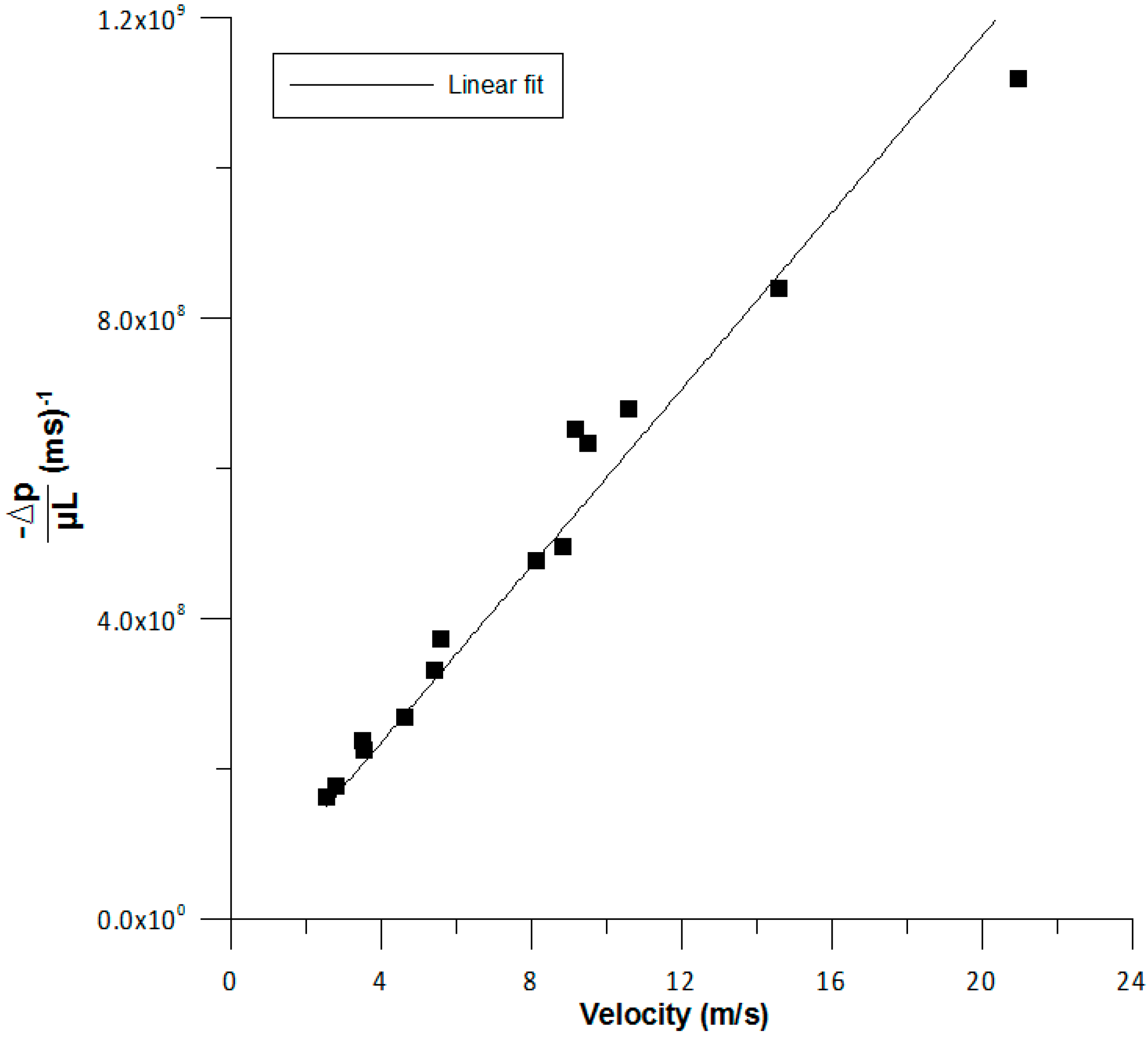
Regarding pressure drop, the linear correlation fits the data appropriately but for high velocities, the deviation can be larger (as seen in Figure 9).

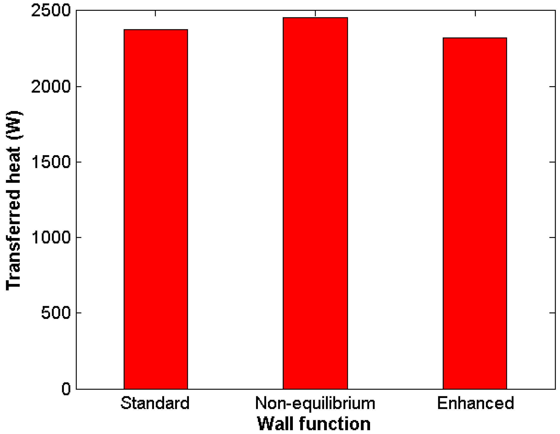
Complex numerical schemes and boundary layer refinement were proven not necessary to obtain reliable results. Standard wall-functions showed good results in comparison with other, more demanding approaches.

4.2. Energy Recovery Considerations for Exhaust Systems

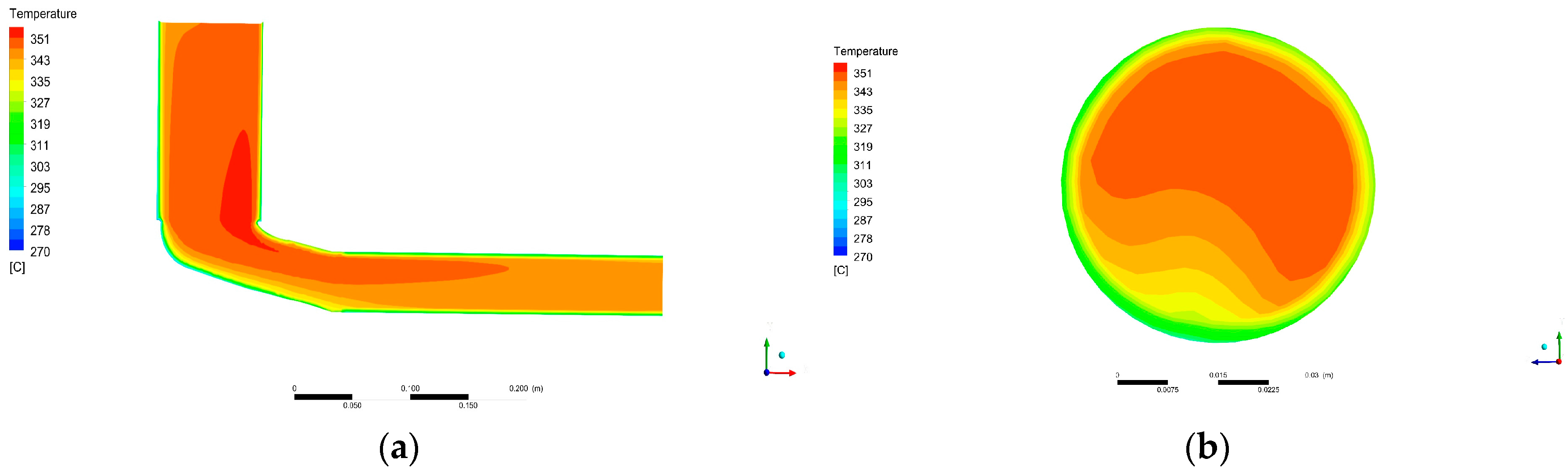
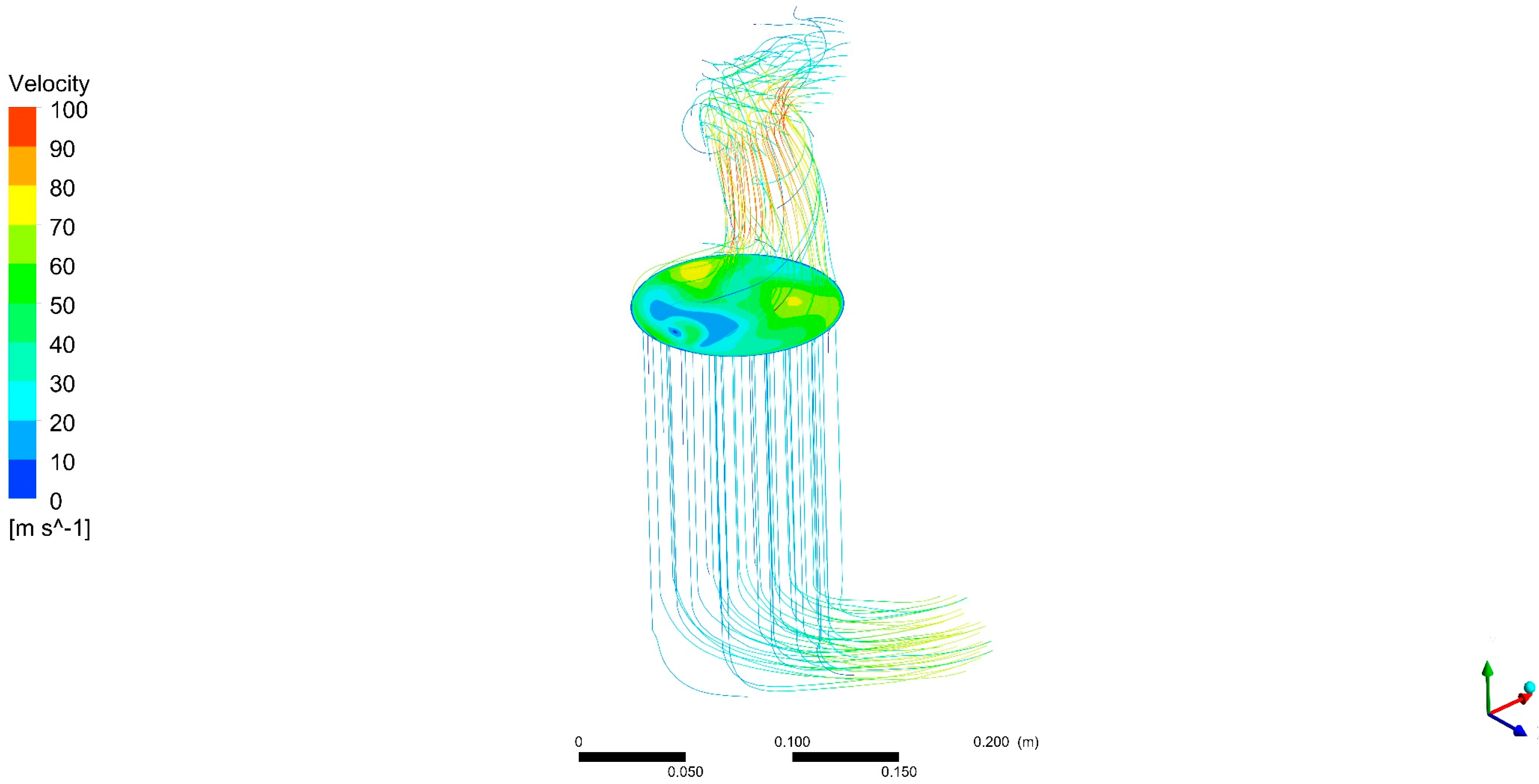
DOC outlet flow analysis showed that modules in thermoelectric generator devices placed after catalytic converters may have different performances not only because of the internal design of the devices but also because of the nature of the exhaust flow. It was found that the smaller the flow, the more uneven the flow temperature distribution is.

This can affect recovery devices being placed in the exhaust system. For instance, modules in a thermoelectric generator expected to have the same behaviour (for instance, upper and lower part thermoelectric modules in a flat-shaped, symmetrical design) may show a different performance due to exhaust flow structures.

Awareness of this effect be used to allow for electrical connections between modules depending on differences in voltage output from modules caused by variations in temperature. Even various types of modules can be selected in each zone to optimize the power output result for the different ranges of temperature.

Loss in gas temperature with distance from DOC outlet was quantified. This will help to assess the trade-off between placing the recovery device near after-treatment systems (higher temperatures) or not (easiness in installation). Notice that temperature falls fast in a relatively short distance, reducing the amount of achievable harvested power.

5. Conclusions

Experimental exhaust data obtained for most common light-duty diesel engines was used to construct a 3D model. A complete methodology to build 3D CFD exhaust models is presented, including how to estimate main parameters needed and numerical approaches. A 2D axi-symmetrical complementary model was shown to be useful to overcome the necessity of chemical parameters fitted to a specific model of catalytic converter.

A computational model incorporating these findings will lead to accurate and faster numerical calculations of analysis of recoverable energy in exhaust systems. This will allow more designs to be explored in a given time.

It has been pointed out that the particular nature of the exhaust flow leaving catalytic converters has to be taken into account for energy-harvesting calculations, since the end of after-treatment systems is the indicated position to place energy recovery devices.

Furthermore, temperature losses caused by placing the recovery device distant from the DOC were evaluated. This information can be used in the evaluation process of the position of a recovery device in an automotive exhaust system. Since temperature falls promptly, it is advised to place the device as close as possible.

In works regarding simulations of recovery devices, if not enough experimental information is available, it is encouraged to include upstream elements of the exhaust that could alter the flow significantly in order to better predict their performance when installed in vehicles.

References

1. Hossain, S.N.; Bari, S. Waste heat recovery from exhaust of a diesel generator set using organic fluids. Procedia Eng. 2014, 90, 439–444. [Google Scholar] [CrossRef]
2. Galindo, J.; Dolz, V.; Royo-Pascual, L.; Haller, R.; Melis, J. Modeling and Experimental Validation of a Volumetric Expander Suitable for Waste Heat Recovery from an Automotive Internal Combustion Engine Using an Organic Rankine Cycle with Ethanol. Energies 2016, 9, 279. [Google Scholar] [CrossRef]
3. Zhang, X.; Romzek, M. Computational Fluid Dynamics (CFD) Applications in Vehicle Exhaust System. SAE Tech. Pap. 2008. [Google Scholar] [CrossRef]
4. Konstantinidis, P.A.; Koltsakis, G.C.; Stamatelos, A.M. Transient heat transfer modelling in automotive exhaust systems. Proc. Inst. Mech. Eng. C J. Mech. Eng. Sci. 1997, 211, l–15. [Google Scholar] [CrossRef]
5. Kandylas, I.P.; Stamatelos, A.M. Engine exhaust system design based on heat transfer computation. Energy Convers. Manag. 1999, 49, 1057–1072. [Google Scholar] [CrossRef]
6. Guardiola, C.; Dolz, V.; Pla, B.; Mora, J. Fast estimation of diesel oxidation catalysts inlet gas temperature. Control Eng. Pract. 2016, 56, 148–156. [Google Scholar] [CrossRef]
7. Shayler, P.J.; Hayden, D.J.; Ma, T. Exhaust System Heat Transfer and Catalytic Converter Performance. SAE Tech. Pap. 1999. [Google Scholar] [CrossRef]
8. Kapparos, D.J.; Foster, D.E.; Rutland, C.J. Sensitivity Analysis of a Diesel Exhaust System Thermal Model. SAE Tech. Pap. 2004. [Google Scholar] [CrossRef]
9. Fu, H.; Chen, X.; Shilling, I.; Richardson, S. A One-Dimensional Model for Heat Transfer in Engine Exhaust Systems. SAE Tech. Pap. 2005. [Google Scholar] [CrossRef]
10. Fortunato, F.; Caprio, M.; Oliva, P; D’Aniello, G.; Pantaleone, P.; Andreozzi, A; Manca, O. Numerical and Experimental Investigation of the Thermal Behavior of a Complete Exhaust System. SAE Tech. Pap. 2007. [Google Scholar] [CrossRef]
11. Chuchnowski, W; Tokarczyk, J; Stankiewicz, K.; Woszczynski, M. Method for modelling temperature distribution in exhaust system of diesel engine in the light of mine systems of heat recuperation. J. KONES Powertrain Transp. 2001, 18, 101–108. [Google Scholar]
12. Guoquan, X. Transient simulation of heat transfers for vehicle exhaust system. In Proceedings of the 7th International Conference on Fluid Mechanics, Qingdao, China, 24–27 May 2015. [Google Scholar]
13. Durat, M.; Parlak, Z.; Kapsiz, M.; Parlak, A.; Fiçici, F. CFD and experimental analysis on thermal performance of exhaust system of a spark ignition engine. J. Therm. Sci. Technol. 2013, 33, 89–99. [Google Scholar]
14. Liu, X. Experiments and simulations on heat exchangers in thermoelectric generator for automotive application. Appl. Therm. Eng. 2014, 71, 364–370. [Google Scholar] [CrossRef]
15. Hamedi, M.R.; Tsolakis, A.; Herreros, J.M. Thermal Performance of Diesel Aftertreatment: Material and Insulation CFD Analysis. SAE Tech. Pap. 2014. [Google Scholar] [CrossRef]
16. Fernández-Yáñez, P.; García-Contreras, R.; Gutiérrez, J.; Agudelo, A.F. Potential for energy recovery from heat transfer rate through the exhaust pipe wall in a light duty diesel engine. In Proceedings of the Energy and Environment Knowledge Week, Paris, France, 28–29 October 2016. [Google Scholar]
17. Voltz, S.E.; Morgan, C.R.; Liederman, D.; Jacob, S.M. Kinetic Study of Carbon Monoxide and Propylene Oxidation on a Platinum Catalyst. Ind. Eng. Chem. Prod. Res. Dev. 1973, 12, 294–301. [Google Scholar] [CrossRef]
18. Oh, S.H.; Cavendish, J.C. Transients of Monolithic Catalytic Converters: Response to Step Changes in Feedstream Temperature as Related to Controlling Automobile Emissions. Ind. Eng. Chem. Prod. Res. Dev. 1982, 21, 29–37. [Google Scholar] [CrossRef]
19. Dubien, C.; Schweich, D.; Mabilon, G.; Martin, B.; Prigent, M. Three-way catalytic converter modelling: Fast- and slow-oxidizing hydrocarbons, inhibiting species, and steam-reforming reaction. Chem. Eng. Sci. 1998, 53, 471–481. [Google Scholar] [CrossRef]
20. Koltsakis, G.C.; Konstantinidis, P.A.; Stamatelos, A.M. Development and Application Range of Mathematical Models for 3-way Catalytic Converters. Appl. Catal. B Environ. 1997, 12, 161–191. [Google Scholar] [CrossRef]
21. Wurzenberger, J.; Wanker, R.; Schüßler, M. Simulation of Exhaust Gas Aftertreatment Systems—Thermal Behavior During Different Operating Conditions. SAE Tech. Pap. 2008. [Google Scholar] [CrossRef]
22. Guojian, W.; Song, T. CFD Simulation of the effect of upstream flow distribution on the light-off performance of a catalytic converter. Energy Convers. Manag. 2005, 46, 2010–2031. [Google Scholar] [CrossRef]
23. Hayes, R.E.; Fadic, A.; Mmbaga, J.; Najaf, A. CFD modelling of the automotive catalytic converter. Catal. Today 2012, 188, 94–105. [Google Scholar] [CrossRef]
24. Chatterjee, D.; Deutschamnn, O.; Warnatz, J. Detailed surface reaction mechanism in a three-way catalyst. Faraday Discuss. 2001, 119, 371–384. [Google Scholar] [CrossRef]
25. Kumar, R.; Sonthalia, A; Goel, R. Experimental study on waste heat recovery from an internal combustion engine using thermoelectric technology. Therm. Sci. 2011, 15, 1011–1022. [Google Scholar] [CrossRef]
26. Pong, H; Wallace, J.; Sullivan, P.E. Modeling of Exhaust Gas Treatment for Stationary Applications. SAE Tech. Pap. 2012. [Google Scholar] [CrossRef]
27. Cárdenas, M.D.; Armas, O; Mata, C; Soto, F. Performance and pollutant emissions from transient operation of a common rail diesel engine fueled with different biodiesel fuels. Fuel 2016, 185, 743–762. [Google Scholar]
28. Cárdenas, M.D. Estudio de las Emisiones de Motores Diésel de Automoción en Condiciones de Funcionamiento Transitorias al Usar Biodiesel. Ph.D. Thesis, Universidad de Castilla-La Mancha, Albacete, Spain, 2016. (In Spanish). [Google Scholar]
29. Dullien, F.A. Porous Media–Fluid Transport and Pore Structure; Academic: New York, NY, USA, 1979. [Google Scholar]
30. Andrade, J.S.; Costa, U.M.S.; Almeida, M.P.; Makse, H.A.; Stanley, H.E. Inertial Effects on Fluid Flow through Disordered Porous Media. Phys. Rev. Lett. 1999, 82, 5249–5252. [Google Scholar] [CrossRef]
31. Benjamin, S.F.; Liu, Z.; Roberts, C.A. Automotive catalyst design for uniform conversion efficiency. Appl. Math. Model. 2004, 28, 559–572. [Google Scholar] [CrossRef]
32. Mladenov, N.; Koop, J.; Tischer, S.; Deutschmann, O. Modeling of transport and chemistry in channel flows of automotive catalytic converters. Chem. Eng. Sci. 2010, 65, 812–826. [Google Scholar] [CrossRef]
33. Patankar, S.V.; Spalding, D.B. A calculation procedure for heat, mass and momentum transfer in three-dimensional parabolic flows. Int. J. Heat Mass Transf. 1972, 15, 1787–1806. [Google Scholar] [CrossRef]
34. Shih, T.; Liou, W.W.; Shabbir, A.; Yang, Z.; Zhu, J. A New k-e Eddy-Viscosity Model for High Reynolds Number Turbulent Flows—Model Development and Validation. Comput. Fluids 1995, 24, 227–238. [Google Scholar] [CrossRef]
35. Agudelo, A.F.; García-Contreras, R.; Agudelo, J.R.; Armas, O. Potential for exhaust gas energy recovery in a diesel passenger car under European driving cycle. Appl. Energy 2016, 174, 201–212. [Google Scholar] [CrossRef]
36. Vazquez, J.; Sanz-Bobi, M.A.; Palacios, R.; Arenas, A. State of the art of thermoelectric generators based on heat recovered from the exhaust gases of automobiles. In Proceedings of the 7th European Workshop on Thermoelectrics, Pamplona, Spain, 3–4 October 2002. [Google Scholar]
37. Launder, B.E.; Spalding, B.I. The numerical computation of turbulent flows. Comput. Methods Appl. Mech. Eng. 1974, 3, 269–289. [Google Scholar] [CrossRef]
38. Incropera, F.P.; DeWitt, D.P. Introduction to Heat Transfer; John Wiley & Sons: New York, NY, USA, 2011. [Google Scholar]
Figure 1. View of the engine test bench including (a) the exhaust system pipe and (b) the diesel oxidation catalyst (DOC).
Applsci 07 00590 g001
Figure 2. Sketch of the exhaust with measurement points involved in the development of the model. The exhaust system is 4 m long and pipe has a diameter of 5 cm (figure not to scale).
Applsci 07 00590 g002
Figure 3. Test matrix. Circles represent selected engine operating points.
Applsci 07 00590 g003
Figure 4. Example of infrared images of the exhaust line in (a) the exhaust pipe and (b) the DOC. Temperatures in the scale are in °C. Squares seen in (a) are wall temperature measurement points.
Applsci 07 00590 g004
Figure 5. Geometry of the 2D axisymmetric DOC model for the tuning process of kinetic parameters. Darker shade of grey represents the monolith.
Applsci 07 00590 g005
Figure 6. Three-dimensional geometry model of the exhaust system.
Applsci 07 00590 g006
Figure 7. Mesh detail. Tetrahedral (DOC inlet and outlet cones) and hexahedral zones (monolith and pipe) can be distinguished.
Applsci 07 00590 g007
Figure 8. Results of test runs with different wall functions. No great disagreement between the three approaches was obtained.
Applsci 07 00590 g008
Figure 9. Plot for viscous resistance derivation. Linear fit constant: B = 5.9 × 10⁷ m−2.
Applsci 07 00590 g009
Figure 10. Plot for (a) CO kinetic parameters derivation. Linear fit: CCO = 21.261, DCO = 5685.10 K (b) C3H6 kinetic parameters derivation Linear fit: CC3H6 = 14.647, DC3H6 = 2388.55 K.
Applsci 07 00590 g010
Figure 11. Streamlines and inlet velocity distribution in the monolith. An example of usual bad flow uniformity caused by inlet cones in automotive catalysts can be seen.
Applsci 07 00590 g011
Figure 12. Temperature distribution for the 2400 rpm–110 Nm mode in (a) monolith, outlet cone and exhaust pipe and (b) cross-section of DOC outlet (before exhaust pipe).
Applsci 07 00590 g012
Figure 13. Plot for coefficient of variation in temperature distribution at DOC outlet. White dots represent engine modes in which chemical processes were not active.
Applsci 07 00590 g013