Article

A TSVD-Based Method for Forest Height Inversion from Single-Baseline PolInSAR Data

School of Geosciences and Info-Physics, Central South University, Changsha 410083, China
*
Author to whom correspondence should be addressed.
Appl. Sci. 2017, 7(5), 435; https://doi.org/10.3390/app7050435
Submission received: 28 January 2017 / Revised: 20 April 2017 / Accepted: 21 April 2017 / Published: 25 April 2017
(This article belongs to the Special Issue Polarimetric SAR Techniques and Applications)

Abstract

:
The random volume over ground (RVoG) model associates vegetation vertical structure parameters with multiple complex interferometric coherence observables. In this paper, on the basis of the RVoG model, a truncated singular value decomposition (TSVD)-based method is proposed for forest height inversion from single-baseline polarimetric interferometric synthetic aperture radar (PolInSAR) data. In addition, in order to improve the applicability of TSVD for this issue, a new truncation method is proposed for TSVD. Differing from the traditional three-stage method, the TSVD-based inversion method estimates the pure volume coherence directly from the complex interferometric coherence, and estimates the forest height from the estimated pure volume coherence with a least-squares method. As a result, the TSVD-based method can adjust the contributions of the polarizations in the estimation of the model parameters and avoid the null ground-to-volume ratio assumption. The simulated experiments undertaken in this study confirmed that the TSVD-based method performs better than the three-stage method in forest height inversion. The TSVD-based method was also applied to E-SAR P-band data acquired over the Krycklan Catchment, Sweden, which is covered with mixed pine forest. The results showed that the TSVD-based method improves the root-mean-square error by 48.6% when compared to the three-stage method, which further validates the performance of the TSVD-based method.

1. Introduction

It is well known that vegetation height plays an important role in quantifying the terrestrial carbon cycle [1,2]. Moreover, vegetation height is an essential factor for the estimation of the biomass stored in vegetation [3,4]. Therefore, accurately extracting vegetation height at a large scale is an important task. Given the fact that polarimetric interferometric synthetic aperture radar (PolInSAR) can separate the scattering power of a single resolution cell into the contributions of surface, double-bounce, and volume scattering, it can be considered to be a viable remote sensing technique for estimating vegetation height in large-scale areas [4,5,6,7,8,9].
PolInSAR can be used to extract vegetation height through its sensitivity to the vegetation vertical structure [10,11,12,13,14]. The complex interferometric coherence of the observed PolInSAR data has been related to the vertical distribution of the vegetation scattering [10,11,12]. In a number of PolInSAR campaigns, the random volume over ground (RVoG) model [6,10] has been used to extract vegetation height from the complex interferometric coherence [15,16,17]. The RVoG model is a physical PolInSAR model that integrates the complex coherence and the biophysical parameters. Based on the RVoG model, Papathanassiou [6] proposed six-dimensional nonlinear optimization method, which has been successfully evaluated with different types of PolInSAR data [6,15,16]. However, for this method, the accuracy of the solution is greatly dependent on the selected initial value, and a poor choice of initial value can result in unstable parameter estimation. Furthermore, the iterative procedure used in this method consumes too much time and is unsuitable for the inversion of large-scale areas. To cope with this problem, Cloude [18] separated the six-dimensional nonlinear parameter optimization process into three stages. This solution is known as the “three-stage method”, and has been widely used in vegetation height extraction for its simple, universal, and time-saving properties [15,19]. However, the three-stage method assumes that there is at least one polarization channel without a ground scattering contribution (the null ground-to-volume ratio (GVR) assumption), and thus it is difficult to determine the polarization because the volume and ground scattering contributions are always mixed in all of the polarization channels due to the diverse penetration depths [20]. As a result, the pure volume coherence estimated by the three-stage method is often inaccurate. Furthermore, with the three-stage method, it is not possible to adjust the contributions of the interferometric coherence observations in the estimation of the RVoG model parameters.
The aim of this work is to address the limitations described above and extract accurate vegetation heights from single-baseline PolInSAR data. Based on the RVoG model, linear observation equations are first developed from the complex interferometric coherence observations by Taylor expansion, in order to combine all the available interferometric coherence observations. Next, since the coefficient matrix derived from the linear equations is ill-conditioned, in order to overcome this ill-posed problem, the proposed truncated singular value decomposition (TSVD)-based method is used to estimate the pure volume coherence. Furthermore, due to the fact that the ordinary truncation method for TSVD is not suitable for this issue, a more adaptive truncation method is proposed so as to improve the accuracy of the estimated pure volume coherence. Finally, the forest height is extracted from the estimated pure volume coherence by the use of a least-squares method.
This paper is structured as follows. The principle of the RVoG model is introduced and discussed in Section 2. Section 3 presents the TSVD-based method for the estimation of vegetation height from complex interferometric coherence observations. The validation of the experiments are presented in Section 4. The discussions are presented in Section 5. Finally, the conclusions are drawn in Section 6.

2. RVoG Model

The RVoG model is a physical model that associates vegetation vertical structure parameters with multiple complex interferometric coherence observables [10]. It is a basic and popular model for describing vegetation scenarios. The model depicts the vegetation layer as a volume with randomly oriented particles over an impenetrable ground surface. Without considering the temporal decorrelation, the complex interferometric coherence γ ( ω ) is expressed as [6]:
γ ( ω ) = e i φ 0 γ v + μ ( ω ) 1 + μ ( ω ) ,
where ω is the unitary polarization vector that defines the choice of scattering mechanism, φ 0 denotes the ground surface phase, μ ( ω ) represents the ground-to-volume ratio (GVR) accounting for the polarization diversity, which varies with ω , and γ v denotes the pure volume coherence, which is linked to the vegetation height and is expressed as [6]:
γ v = 2 σ ( e ( 2 σ h v / cos θ + i k z h v ) 1 ) ( 2 σ + i k z cos θ ) ( e ( 2 σ h v / cos θ ) 1 ) ,
where σ denotes the mean extinction coefficient, h v denotes the vegetation height, θ is the incidence angle, and k z is the vertical wave number, which depends on the imaging geometry and wavelength [21]. k z is given as:
k z = 4 π Δ θ λ sin θ ,
where λ denotes the wavelength, and Δ θ represents the incidence angle difference between the master and slave images.
According to Equation (1), the theoretical loci of the complex coherence sets of different polarizations follow a straight line in the complex plane, as shown in Figure 1 [18]. The figure also depicts the determination of the ground surface phase, which is applied in the three-stage method. However, the complex coherence observations no longer follows a common straight line in practice, due to the coherence fluctuations caused by all the possible decorrelations. In order to reconstruct the straight line accurately from noisy coherence sets, a line-fit approach based on least squares is proposed by the use of the following regression model [10,18]:
Im ( γ ( ω ) ) = c Re ( γ ( ω ) ) + d ,
where Re ( ) and Im ( ) denote the real and imaginary operations, respectively, c is the slope of the coherence line, and d is the intersection point to the imaginary axis. Once more than two complex coherence observations are provided, the coherence line can be determined by the line-fit approach. The ground phase φ 0 can then be identified by the two intersections ( φ 1 and φ 2 ) of the coherence line and the unit circle [18]. However, the least-squares criterion may be unstable if the ellipticity of the coherence sets is high or if the complex coherence observations are too discrete, due to the noise of the polarizations.
In addition, the three-stage method assumes that there is a polarization channel without ground scattering contribution, i.e., μ ( ω ) = 0 , and then uses this assumption to further estimate the pure volume coherence. However, the volume and ground scattering contributions are always mixed in the polarization channels due to the diverse penetration depths. Therefore, it is difficult to find a polarization that can fit this hypothesis. As a result, when relying on this assumption, the estimated pure volume coherence will bias the extracted forest height.
As shown in Equation (1), γ ( ω ) is polarization-dependent. The complex coherence observations of the different scattering mechanisms can be obtained by the use of different unitary polarization vectors ω . In other words, if the number of polarization vectors is m, then m equations like Equation (1) can be established. By using the least-squares criterion, the unknown parameters in γ ( ω ) can be estimated when the number of parameters is less than that of the equations. Therefore, the least-squares method is a viable way to estimate vegetation height from complex coherence observations. The least-squares method directly estimates the RVoG model parameters from the complex coherence observations without any assumptions, and it is able to adjust the contributions of the coherence observations in the estimation of the model parameters.

3. The TSVD-Based Method for the Estimation of Vegetation Height From Complex Interferometric Coherence Observations

In this section, a novel approach is introduced for the estimation of vegetation height from single-baseline PolInSAR data, on the basis of the least-squares criterion and the TSVD-based method.

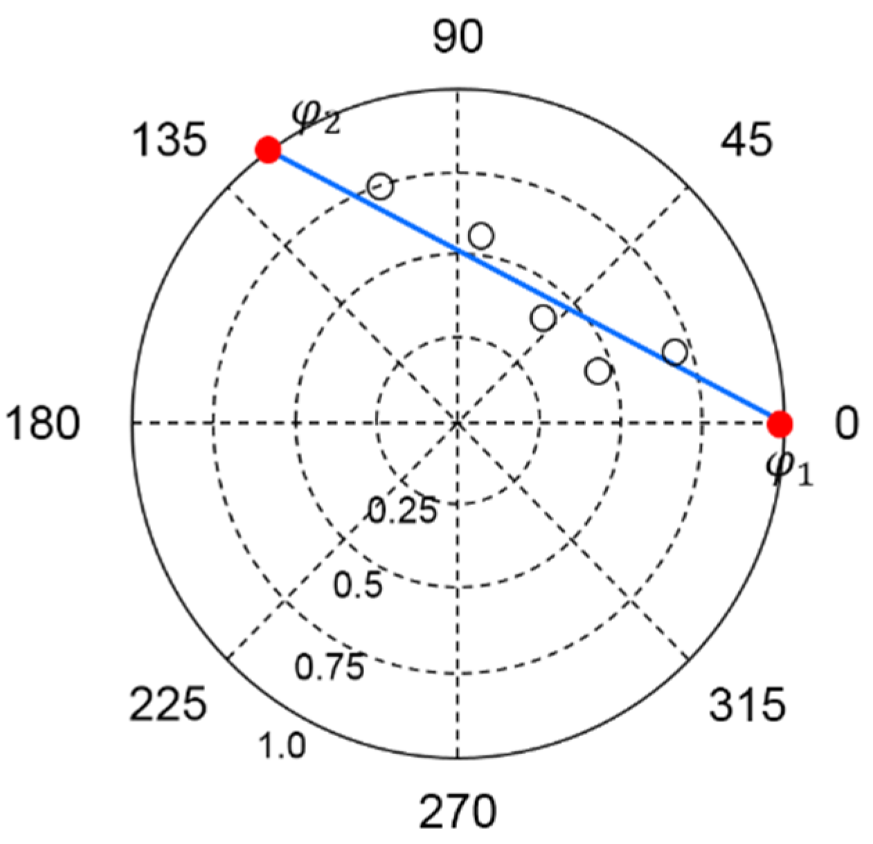
3.1. Estimation of Pure Volume Coherence from the Complex Interferometric Coherence Observations

From Equations (1) and (2), it can be seen that γ ( ω ) and γ v are complex numbers. Therefore, the equations can be separated into two parts: a real part and an imaginary part. In order to simplify the nonlinear equations, we parameterize the pure volume coherence by γ v = a + b i , and then the complex interferometric coherence can be given by:
γ ( ω ) = e i φ 0 a + b i + μ ( ω ) 1 + μ ( ω ) ,
and the observational function for the least-squares criterion can be formulated as:
γ ( ω j ) = f ( φ 0 , a , b , μ ( ω j ) ) j = 1 , 2 , , m ,
where ω j is the j-th unitary polarization vector, f is the RVoG model function, as described in Equation (5), μ ( ω j ) is the j-th GVR associated with vector ω j , and m represents the number of polarization projection vectors. It is clear that there are four unknown model parameters in each function, and m + 3 unknown parameters in m functions.
To estimate the unknown model parameters, least-squares estimation is adopted to adjust the contributions of the complex coherence observations and suppress noise [20,22,23]. The corresponding least-squares criterion can be formulated as:
j = 1 m | γ ^ ( ω j ) γ ( ω j ) | 2 = min ,
where represents the summation operation, | · | represents the modulus operation, and γ ^ ( ω j ) is the estimation of γ ( ω j ) . Since the complex coherence can be separated into a real part and an imaginary part, Equation (7) can be equally converted to:
j = 1 m ( | Re ( γ ^ ( ω j ) ) Re ( γ ( ω j ) ) | 2 + | Im ( γ ^ ( ω j ) ) Im ( γ ( ω j ) ) | 2 ) = min .
In this way, the residual functions for the least-squares criterion are formulated as:
{ V Re j = Re ( γ ^ ( ω j ) ) Re ( γ ( ω j ) ) , V Im j = Im ( γ ^ ( ω j ) ) Im ( γ ( ω j ) ) ,
where V Re j denotes the residual of the real part corresponding to the j-th unitary polarization vector, and V Im j denotes the residual of the imaginary part. From Equation (9), it can be seen that, if the number of polarization projection vectors is m, then 2m residual equations can be established. The number of unknown parameters is m + 3. Therefore, the unknowns can be estimated by least-squares estimation when the number of polarization projection vectors is more than three.
From Equation (5), it can be seen that the complex coherence function is highly nonlinear, which greatly affects the efficacy of the least-squares estimation. In view of this, a linearized strategy based on a Taylor series is adopted to convert the nonlinear function into a linear function [23]. In this case, the residual functions for the least-squares criterion can be rewritten as:
{ V Re j = Re ( γ ( ω j ) ) φ 0 d φ 0 + Re ( γ ( ω j ) ) a d a + Re ( γ ( ω j ) ) b d b + Re ( γ ( ω j ) ) μ ( ω j ) d μ ( ω j ) l Re j V Im j = Im ( γ ( ω j ) ) φ 0 d φ 0 + Im ( γ ( ω j ) ) a d a + Im ( γ ( ω j ) ) b d b + Im ( γ ( ω j ) ) μ ( ω j ) d μ ( ω j ) l Im j
where represents the partial derivative operation, d φ 0 , d a , d b , and d μ ( ω j ) denote the corrections of the approximations of the unknown parameters, and l Re j and l Im j are the real and imaginary differences between the observed complex coherence and the predicted initial value. The vector V denotes the residuals, X denotes the unknown corrections, A denotes the coefficient matrix, and L denotes the real and imaginary differences. The residual functions for the least-squares criterion can then be expressed as [23,24]:
V = A X L .
The unitary polarization vector can be constructed by linear-basis polarization, Pauli-basis polarization, magnitude diversity optimization polarization [6], and phase diversity polarization [25]. Therefore, more than three polarization projection vectors can be obtained for the estimation of the unknown parameters. Using the least-squares criterion, an estimate of the unknown corrections can be given by:
X ^ = ( A T A ) 1 A T L ,
where X ^ denotes the estimation of the unknown corrections. The estimation of the model parameters can then be obtained by combining the approximations and the corrections. However, during the computation, we find that matrix A is seriously ill-conditioned. It is well known that an ill-posed problem is a great hindrance to obtaining accurate parameter estimation from observation equations. For an ill-posed equation, a small amount of noise in the observations can often bring large uncertainties to the estimation. The detrimental effect of the ill-posed problem is reflected in the large variance of the least-squares estimations. The variance-covariance matrix of the least-squares estimations can be given by [23]:
Cov X ^ = σ 0 2 ( A T A ) 1 ,
where Cov X ^ represents the variance-covariance matrix of the estimations, and the diagonal elements of the matrix are the variances of the estimations, σ 0 2 denotes the unit weight variance. We perform singular value decomposition (SVD) on matrix A [24]:
A = U S G T ,
S T = [ λ 1 0 0 0 0 0 0 0 0 0 0 λ n 0 0 ] ,
where U is a 2 m × 2 m orthogonal matrix of the left singular vectors, G is an n × n orthogonal matrix of the right singular vectors, and n denotes the number of unknowns, which is equivalent to m + 3, S is the matrix of singular values, and λ are non-negative real numbers that are conventionally listed in decreasing order, i.e., λ 1 > λ 2 > > λ n . Using the trace operation, the sum of the variances of the estimations can be given by:
Vars X ^ = Trace ( Cov X ^ ) = σ 0 2 ( i = 1 n 1 λ i 2 ) ,
where Vars X ^ represents the sum of the variances of the estimations, and Trace denotes the trace operation. If the equation is ill-posed, the singular values gradually decrease to zero, and λ 1 is much larger than λ n ( λ n is close to zero). Equation (16) shows that small singular values greatly magnify the estimation variances. Thus, the least-squares estimation becomes highly unreliable and is unable to obtain accurate estimations of the parameters.
In order to overcome the ill-posedness of the problem, truncated singular value decomposition (TSVD) [26,27,28] is adopted. TSVD truncates the small singular values that greatly enlarge the variances to improve the least-squares estimation. Using the TSVD-based method, the estimation of the unknown parameters is given by:
X ^ t = G S t T U T L ,
S t T = [ S P 1 0 0 S T = 0 0 0 ] ,
where X ^ t denotes the improved estimation by TSVD, S t denotes the inverse singular value matrix which truncates the small singular values, S P is the singular value matrix which represents the preserved large singular values, and S T is a zero matrix that represents the truncated small singular values. We can then obtain the variance of the TSVD estimations as follows:
Vars X ^ t = Trace ( G S t T U T σ 0 2 U S t G T ) = σ 0 2 ( i = 1 k 1 λ i 2 ) ,
where Vars X ^ t represents the variance of the TSVD estimations. k denotes the number of preserved large singular values. Equation (19) shows that TSVD greatly reduces the variance of the least-squares estimations through truncating the small singular values. However, it is well known that TSVD results in a biased estimation. Truncating the small singular values not only reduces the variance but also introduces bias into the estimation. TSVD improves the estimation by reducing the mean-square error (MSE) of the least-squares estimation. The MSE is expressed as [26]:
Mse X ^ t = Vars X ^ t + B i a s X ^ t T Bias X ^ t ,
where Mse X ^ t represents the MSE of the TSVD estimation, and Bias X ^ t represents the bias introduced by TSVD. The sum of squares of Bias X ^ t is given by:
B i a s X ^ t T Bias X ^ t = i = k + 1 n X T G i G i T X ,
where X represents the true values of the unknown parameters, and G i denotes the i-th right singular vector that corresponds to the i-th singular value. Equation (21) shows that the bias is introduced by truncating the small singular values. The more singular values that are truncated, the more bias is introduced. Considering Equation (20), it is clear that TSVD reduces the MSE by truncating the small singular values. However, the reduction of the MSE relies on the reduced variance being more than the introduced bias. Therefore, the truncation parameter k which determines the preserved large singular values and truncated small singular values is a key factor for TSVD to reduce the MSE.
The method that is commonly used for the determination of the truncation parameter is related to the condition number, i.e., λ 1 / λ i , as defined in Equation (15). If the condition number is larger than the given upper limit, the singular value λ i should be truncated [28,29,30]. However, large-scale PolInSAR data usually consist of millions of pixels, and the singular values in ill-conditioned matrices of pixels are different from each other. Therefore, it is difficult to determine a reasonable upper limit for the condition number. In order to determine a reasonable truncation parameter for this issue, we need to develop a new approach. From Equations (19) and (21), it can be seen that if singular value λ i is truncated, the reduced variances are σ 0 2 / λ i 2 and the introduced bias is X T G i G i T X . Therefore, if σ 0 2 / λ i 2 > X T G i G i T X , the singular value should be truncated, and if σ 0 2 / λ i 2 < X T G i G i T X , the singular value should be preserved. In order to determine the small singular values, the values of σ 0 2 / λ i 2 and X T G i G i T X need to be calculated accurately. From the least-squares estimation, the estimation of is given by [23]:
σ ^ 0 2 = V T V 2 m n = ( U U T L L ) T ( U U T L L ) 2 m n ,
where U denotes the 2 m × n dimensional left singular vectors, σ ^ 0 2 is the estimation of σ 0 2 [23,26], and n is the number of unknowns. It is clear that the small singular values have no adverse effect on the estimation of σ 0 2 . Therefore, σ 0 2 / λ i 2 can be calculated by the least-squares solution if 2 m > n [23,26]. In this paper, 10 polarizations are selected for the estimation of the pure volume coherence. Therefore, σ 0 2 can be estimated.
Using the SVD matrices of A , the estimation of G i T X by least squares can be expressed as:
G i T X ^ = λ i 1 U i T L .
It can be seen from Equation (23) that the singular values greatly affect the estimation of G i T X . Small singular values seriously enlarge the value of G i T X ^ , whereas large singular values do not. The variance of the estimation of G i T X can be given by:
Var g = λ i 1 U i T σ 0 2 U i λ i 1 = σ 0 2 λ i 2 ,
where Var g represents the variance of estimation G i T X ^ . The equation shows that the variance of G i T X ^ is negatively correlated with the singular value. Therefore, the variance of G i T X ^ which corresponds to a large singular value is small. Furthermore, the estimation of G i T X is reliable due to the small variance. However, the estimation of G i T X , which corresponds to a small singular value, is unreliable due to the large variance.
Generally, if the standard deviation of G i T X ^ is less than 3 σ ^ 0 , the estimation is considered to be reliable. Therefore, the reliable estimations with a standard deviation of less than 3 σ ^ 0 can be given by J = [ X ^ T G 1 G 1 T X ^ ,   X ^ T G 2 G 2 T X ^ , , X ^ T G j G j T X ^ ] . Since the values of the reduced variances σ ^ 0 2 / λ i 2 change as σ ^ 0 2 / λ 1 2 < σ ^ 0 2 / λ 2 2 < < σ ^ 0 2 / λ n 2 , if σ ^ 0 2 / λ i 2 is bigger than 90% of the values of J , it can be considered that σ 0 2 / λ i 2 > X T G i G i T X , and singular value λ i needs to be truncated. The other small singular values λ r that are smaller than λ i can also be denoted as σ 0 2 / λ r 2 > X T G r G r T X and need to be truncated. The small singular values which should be truncated in the TSVD-based method are thus determined. The ill-posed problem can be well solved by TSVD with the proposed truncation method. Finally, the pure volume coherence can be estimated by the proposed TSVD-based method.

3.2. Extraction of Vegetation Height from the Pure Volume Coherence

Since the pure volume coherence is parameterized by γ v = a + b i , the pure volume coherence is estimated as γ ^ v = a ^ + b ^ i by the proposed TSVD-based method. Using the estimated parameters a ^ and b ^ , the pure volume coherence which links to the vegetation height can be expressed as:
a ^ + b ^ i = 2 σ ( e ( 2 σ h v / cos θ + i k z h v ) 1 ) ( 2 σ + i k z cos θ ) ( e ( 2 σ h v / cos θ ) 1 ) .
The equation can then be separated into a real part and an imaginary part:
{ a ^ = Re ( γ v ) , b ^ = Im ( γ v ) .
From Equation (25), it can be seen that θ and k z are the known parameters, and the unknown parameters are σ and h v . Therefore, σ and h v can be estimated by the least-squares estimation from Equation (26). The Taylor series is used to convert the nonlinear function into a linear function. The residual functions for the least-squares criterion can then be expressed as [23]:
{ V Re p = Re ( γ v ) σ d σ + Re ( γ v ) h v d h v l Re , p V Im p = Im ( γ v ) σ d σ + Im ( γ v ) h v d h v l Im , p
where V Re p denotes the residual of the real part, and V Im p denotes the residual of the imaginary part, d σ and d h v denote the corrections of the approximations of the unknown parameters, and l Re p and l Im p are the real and imaginary differences between the estimated pure volume coherence and the predicted initial value. Using the vector V p to denote the residuals, X p denotes the unknown corrections, A p denotes the coefficient matrix, and L p denotes the real and imaginary differences. The residual functions for the least-squares criterion can then be expressed as [23,24,29]:
V p = A p X p L p .
Since the number of residual equations is the same as that of the unknowns, the least-squares criterion can be used to estimate the unknowns. The estimation is given by:
X ^ p = ( A p T A p ) 1 A p T L p ,
where X ^ p denotes the estimation of the unknowns. The vegetation height can then be obtained from the estimation of d h v and the initial value of h v by:
h ^ v = h v 0 + d h v ,  
where h ^ v denotes the estimated vegetation height, and h v 0 denotes the initial value of h v .

3.3. The Determination of Initial Values of Model Parameters

From Equations (10) and (27), it can be seen that the proposed method is plagued by the initial value. If the initial value cannot be well determined, it is difficult to get reliable estimation. The classical six-dimensional nonlinear optimization method [6] is also confronted by this problem since it is difficult to obtain the priori information of the forest parameters (forest height and extinction). However, it is easy to obtain reliable initial values of the ground phase, the pure volume coherence and the ground-to-volume ratio according to the RVoG assumption and its linear geometrical expression in the complex plane [10]. Based on this, Equation (10) is used to estimate the pure volume coherence, which is important to invert the forest parameters. Compared to the six-dimensional nonlinear optimization method, this method can avoid significant biases caused by the unreliable initial values of forest parameters. Moreover, in comparison to the three-stage method, the proposed method can provide more accurate pure volume coherence because it is free from the assumption that there is one polarization whose ground-to-volume power ratio should be less than −10 dB [10], which cannot be fulfilled for the low-frequency PolInSAR data or for the sparse forest [31]. In addition, only one polarimetric observation is used to calculate the pure volume coherence in the three-stage method. However, multi-polarization observations are used to estimate the pure volume coherence under the TSVD based least-squares estimation framework, which enhances the method's ability to alleviate the effect of observational errors in the estimations. As a result, the obtained pure volume coherence can support more accurate forest parameter estimation.
Then, with the estimated pure volume coherence, Equation (27) is used to estimate forest height. The initial values for the forest height and the mean extinction coefficient are determined by the three-stage method. Although the three-stage method cannot give satisfactory results, especially for the low-frequency PolInSAR data or for sparse forest, these estimated results can be regarded as the initial values for Equation (27). The least-squares method estimates the corrections of initial values from the reliable pure volume coherence to improve the accuracy of the estimated unknown parameters. The final experiment has shown that with the accurate pure volume coherence and reasonable initial values, the proposed method can attain good forest height results.

4. Examples

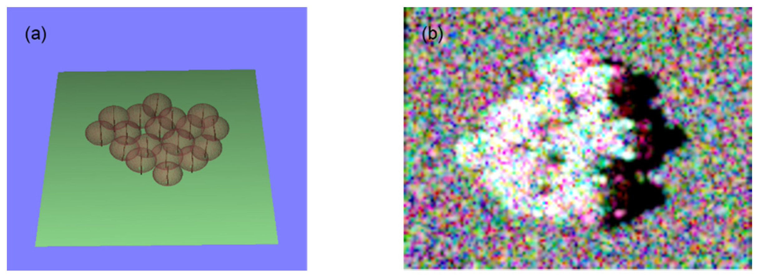
4.1. Simulated Experiments

In order to evaluate the performance of the proposed TSVD-based inversion method for the estimation of vegetation height from single-baseline PolInSAR data, we simulated single-baseline PolInSAR data through the PolSARpro tool released by European Space Agency (ESA), Rome, Italy, using the following forest scenario, as shown in Table 1: simulated broad-leaved forest with an average height of 18 m; and ground phase of 0 degrees, corresponding to a ground elevation of 0 m. The complex interferometric coherence of the linear-basis polarizations (transmitted polarization and received polarization are horizontal polarizations, HH, transmitted polarization and received polarization are vertical polarizations, VV) and the Pauli-basis polarization (transmitted polarization is horizontal polarization and received polarization is vertical polarization, HV) could then be obtained. The simulated forest area and the Pauli RGB composite image are shown in Figure 2.
Furthermore, using Pauli-basis polarization, magnitude diversity optimization polarization [6], and phase diversity polarization [25], the complex interferometric coherence observations of HH+VV, HH-VV, opt1, opt2, opt3, phase diversity (PD)-high, and phase diversity (PD)-low could be obtained. Therefore, 20 residual equations could be established from the above 10 complex interferometric coherence observations based on Equation (10) with 13 unknown parameters. The unknown parameters were then estimated by the TSVD-based method. From the estimated parameters and the pure volume coherence model which links to the forest height, the forest height could be extracted by Equation (29). The extraction results are shown in Figure 3b. For comparison, the extraction results of the three-stage method are shown in Figure 3a.
From Figure 3, it can be seen that the TSVD-based method performs much better than the three-stage method in forest height inversion in this test. Clearly, from Figure 3a, the three-stage method fails to invert the forest heights of the rectangular areas of the figure, but the TSVD-based method effectively improves the inversion of the rectangular areas, as can be seen in Figure 3b. The mean values of the extracted forest heights by the three-stage method and the TSVD-based method are 13.383 m and 15.4440 m. This demonstrates that the forest height estimated by TSVD is more accurate than that estimated by the three-stage method. For a further comparison, 16 forest stands were selected from the simulated forest area, and the root-mean-square error (RMSE) of each stand was adopted to compare the performance of the two methods. The RMSEs of each stand are shown in Figure 4.
For the 16 forest stands, the RMSE of the TSVD-based method is consistently less than that of the three-stage method. This indicates that the inverted forest height obtained by TSVD is closer to the true height than the height obtained by the three-stage method. This further validates the performance of the TSVD-based method.

4.2. Validation with E-SAR P-Band Data

4.2.1. Study Area and Data Sets

The proposed TSVD-based method was also applied to E-SAR P-band PolInSAR data, which were collected under the framework of the BioSAR 2008 campaign by the German Aerospace Center, Munich, Germany. The test site is a forest area within the Krycklan River catchment in Northern Sweden, and is mainly covered by mixed boreal forest with heights ranging from 0 to 35 m. The topography elevation is between 150 to 380 m above mean sea level (AMSL). The baseline PolInSAR data were acquired in the repeat-pass configuration. Moreover, as part of the BioSAR2008 campaign, a light detection and ranging (LiDAR) measurement was also obtained by the Swedish Defense Research Agency (FOI). The derived forest height is regarded as the reference in the following analysis.
In this experiment, the forest heights were extracted from single-baseline data. The temporal and spatial baselines were 70 min and 32 m, respectively. The vertical wavenumber ranged from 0.051 to 0.181.The Pauli-basis RGB composite intensity image for the test site is shown in Figure 5.

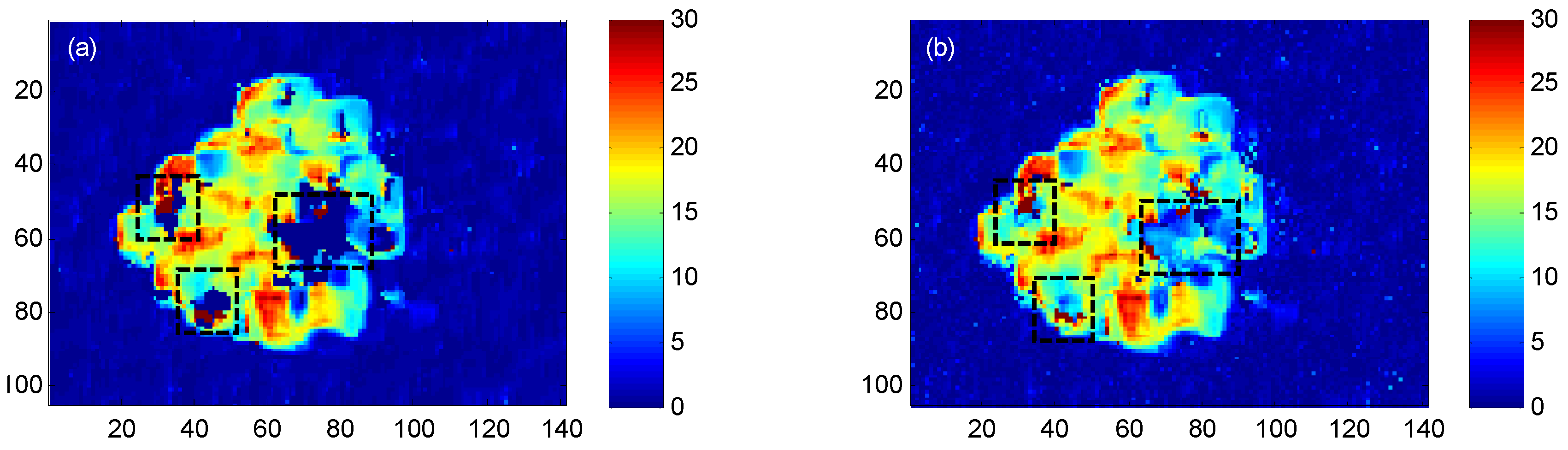
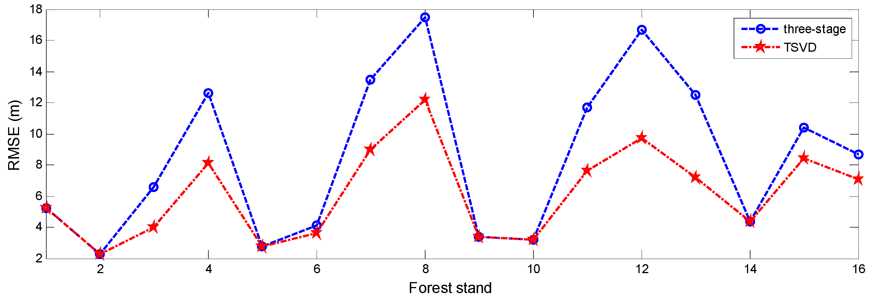
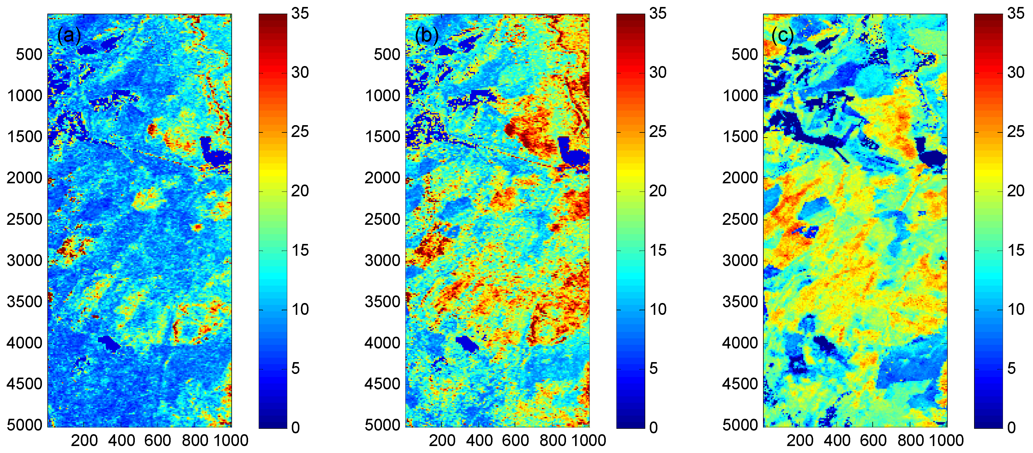
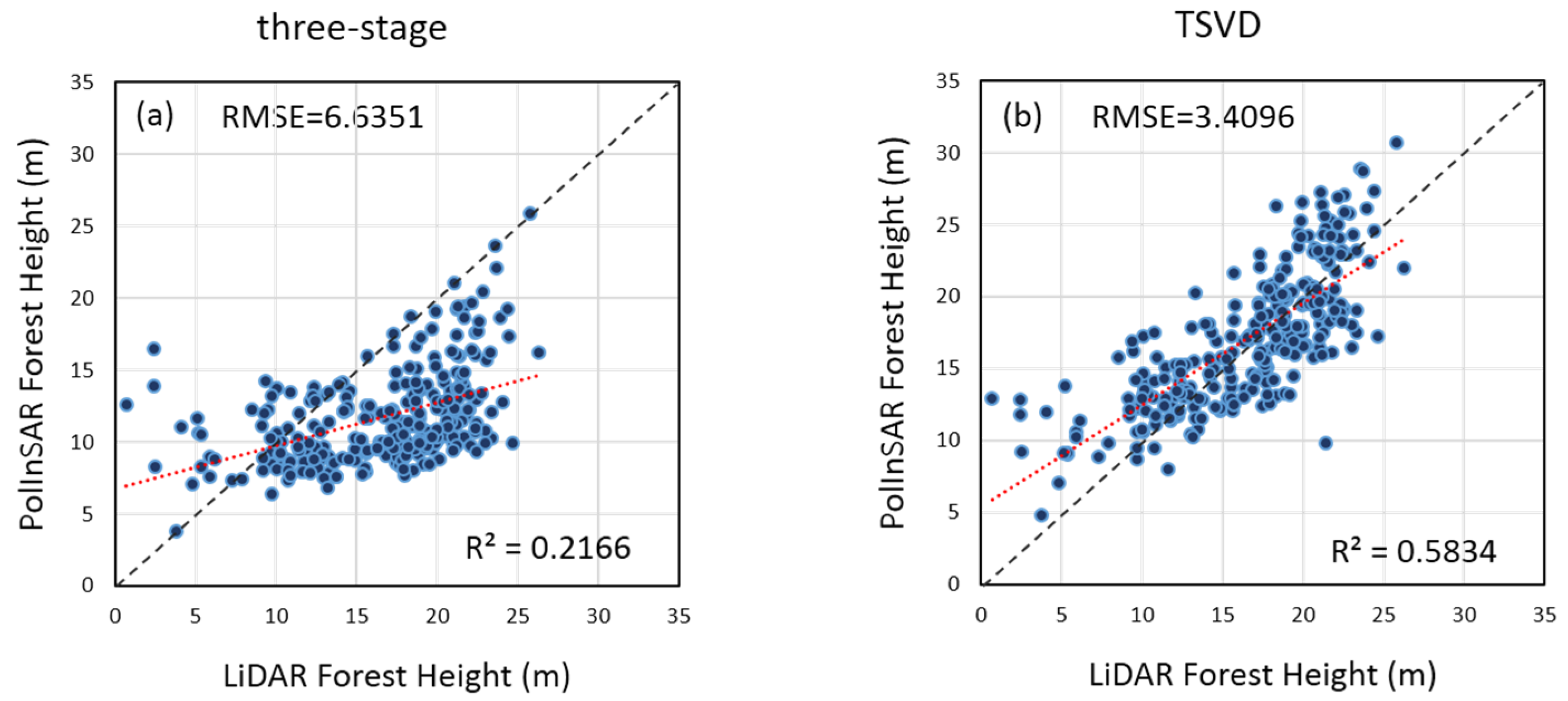
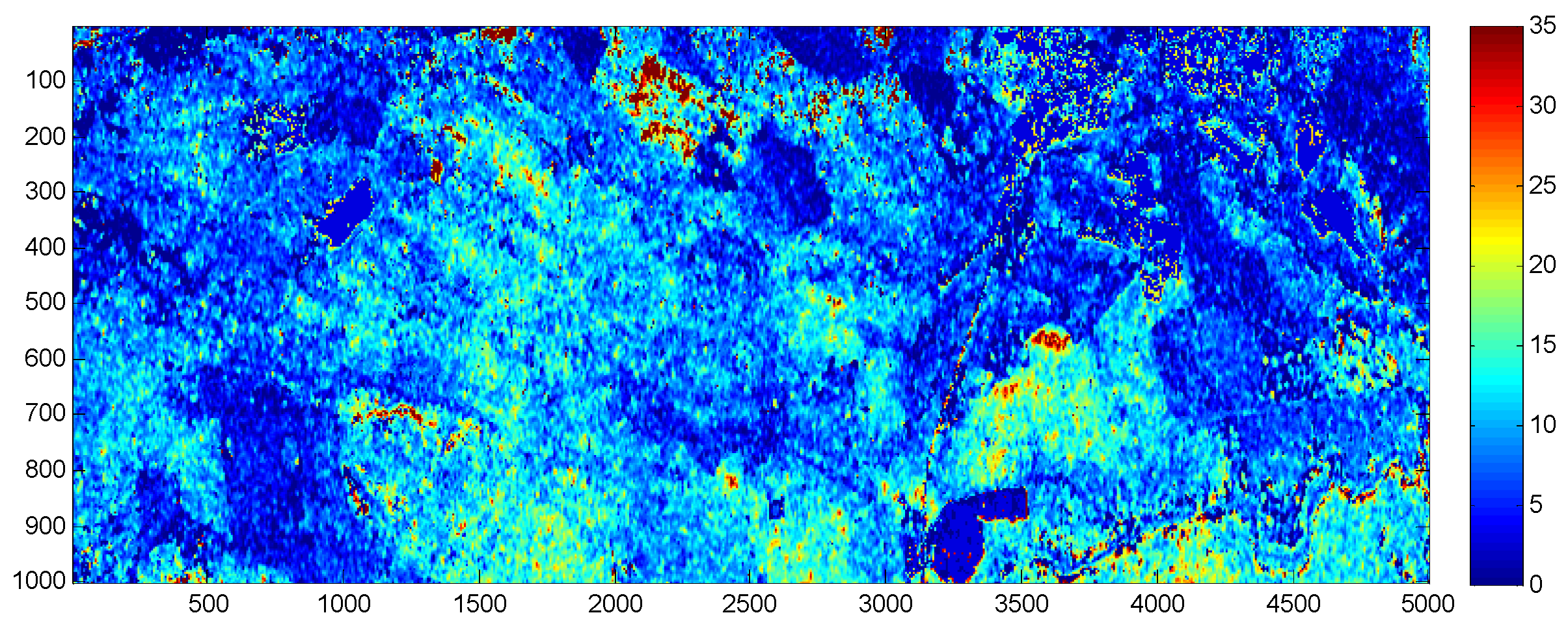
4.2.2. Forest Height Inversion

Following the steps of the TSVD-based inversion method, the complex interferometric coherence observations of HH, VV, HV, HH+VV, HH-VV, opt1, opt2, opt3, PDhigh, and PDlow were used to establish the residual equations. The pure volume coherence was then estimated by the TSVD-based method from the residual equations and, finally, the forest heights were extracted from the pure volume coherence model using the estimated model parameters. The extracted forest heights are shown in Figure 6b. As in the simulated experiments, the three-stage method was also used to extract the forest heights, and the inversion results are shown in Figure 6a. Figure 6c shows the LiDAR forest heights used as a reference.
It can be seen from Figure 6 that the inversion results of the three-stage method and the TSVD-based method follow a similar spatial trend, but significant differences are also apparent. Compared to the LiDAR results, the inverted forest heights obtained by TSVD are clearly more accurate than those of the three-stage method. In order to analyze the differences, 272 forest stands characterized by nearly uniform tree heights were selected from the LiDAR results. We took the estimated forest height average for every stand and computed the difference between that and the LiDAR forest height. The RMSE and correlation coefficient (R2) were calculated to validate the performance. The validated stand-level plots are displayed in Figure 7.
The validated plots of the three-stage method and the TSVD-based method are characterized by R2 values of 0.2166 and 0.5824, respectively. This indicates that the forest heights inverted by TSVD are closer to the LiDAR forest heights. The RMSEs of the three-stage method and TSVD are 6.6351 and 3.4096, respectively. Clearly, the inversion accuracy of TSVD is higher than that of the three-stage method, showing an improvement of 48.6%. Therefore, it is possible to state that the TSVD-based method can improve the inversion of the forest height in this test site.

5. Discussion

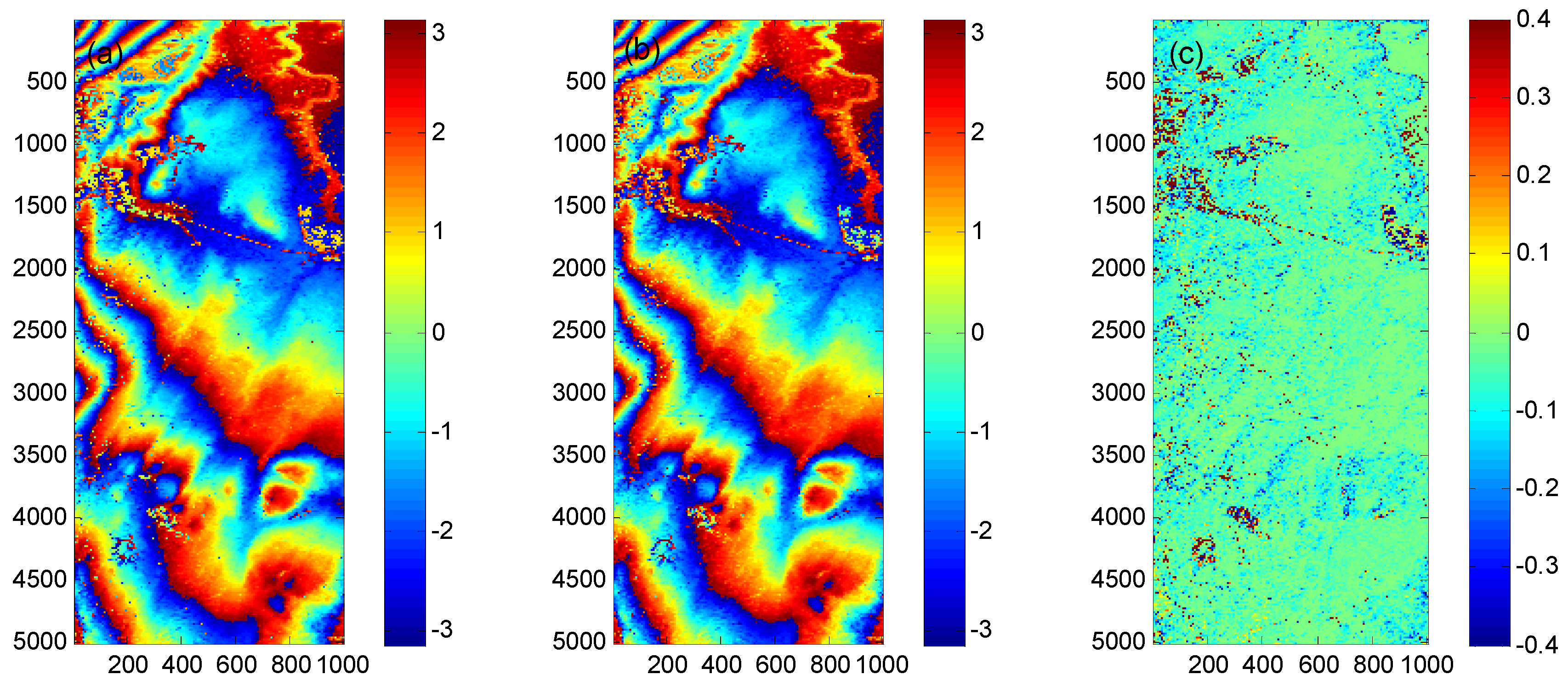
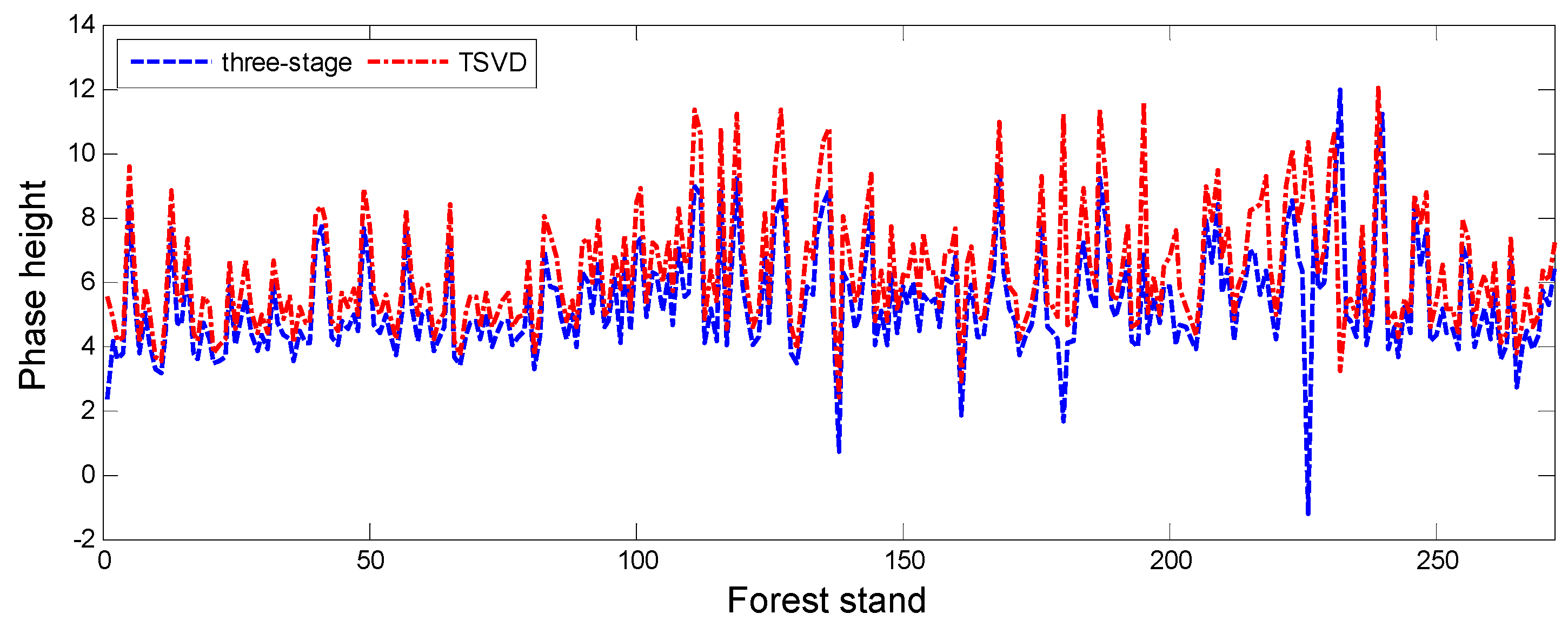
5.1. The Extracted Ground Surface Phases by the Three-Stage Method and TSVD

From Equation (10), it can be seen that the ground surface phase can also be estimated by the TSVD-based method. Since the ground surface phase plays an important part in the estimation of the underlying topography [30,32,33], the extracted ground surface phases obtained by the three-stage method and TSVD are shown in Figure 8a,b, respectively.
It is difficult to see any difference between Figure 8a,b. This indicates that the three-stage method and TSVD perform similarly in extracting the ground surface phase. For a more in-depth analysis, the ground surface phase obtained by TSVD subtracted from that obtained by the three-stage method is shown in Figure 8c. It can be seen that most of the values in Figure 8c are close to zero. This further validates that TSVD is unable to improve the accuracy of the estimation of the ground surface phase and the underlying digital elevation model (DEM) [30].
The line-fit approach is used in the three-stage method to determine the ground surface phase. In order to reconstruct the straight line accurately from noisy coherence sets, 10 polarizations are used by least-squares based line-fit approach. Similarly, the same 10 polarizations are used in TSVD for the estimation of model parameters. Therefore, the observations used by line-fit approach and TSVD have the same noise and information, and the basic criterion in the line-fit approach and TSVD both are least-squares. This is a possible reason for this result.

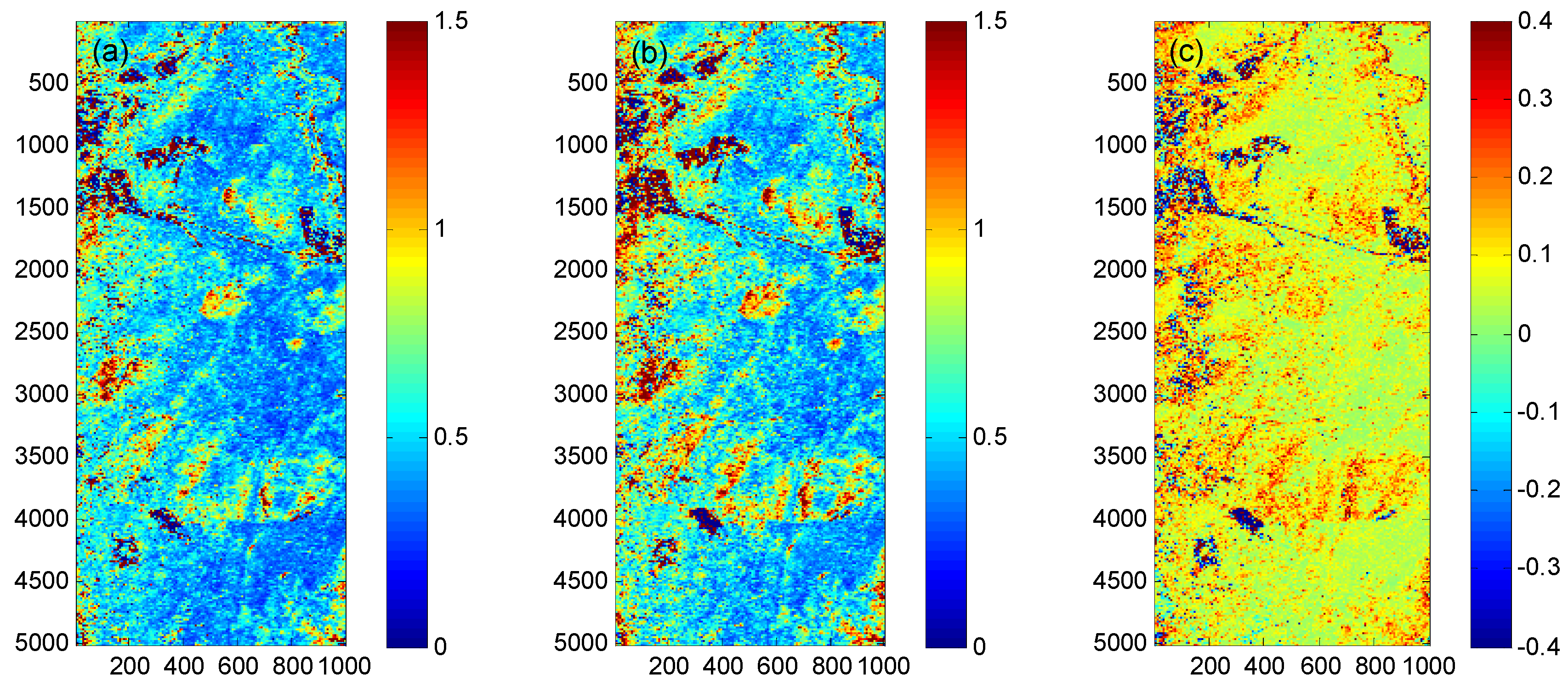
5.2. Effects on Estimation of Phase Height

As mentioned in Section 3, the TSVD-based method first estimates the pure volume coherence from the complex interferometric coherence and then extracts the forest height. The phase height, which is very important for the inversion of forest height [34,35], was also computed from the estimated pure volume coherence and compared with the result of the three-stage method. The phase heights calculated from the estimated pure volume coherence obtained by the three-stage method and TSVD are shown in Figure 9a,b.
From Figure 9a,b, it can be seen that the estimated phase heights in Figure 9a are higher than those in Figure 9b. We subtracted the phase heights in Figure 9b from those in Figure 9a and display the results in Figure 9c. Clearly, most of the values in Figure 9c are positive numbers. This indicates that the phase height extracted by TSVD is a better fit for the theoretical phase height of the pure volume coherence than the phase height extracted by the three-stage method. For a further comparison, we computed the average phase height of each forest stand and show the results in Figure 10.
Figure 10 clearly indicates that the phase heights estimated by the TSVD-based method are consistently higher than those estimated by the three-stage method in each forest stand. Therefore, the forest heights inverted by TSVD are more accurate than those inverted by the three-stage method in the forest stands. To confirm this conclusion, we also used the least-squares method to extract the forest heights from the pure volume coherence estimated by the three-stage method, as mentioned in Section 3.2. The results are shown in Figure 11.
Comparing Figure 11 and Figure 5b, which displays the inversion results of TSVD, clearly, the forest heights in Figure 5b are closer to the LiDAR forest heights than those in Figure 11. Therefore, we can conclude that the TSVD-based method has the capacity to improve the estimation of the pure volume coherence. Based on the improved pure volume coherence, the forest height can be extracted more accurately.

5.3. Limitations of the TSVD-Based Method

Two problems are worth discussing. Firstly, TSVD plays an important role in the proposed solution. Since the ordinary truncation method is not suitable for this issue, a more adaptive truncation method is proposed in this paper. From Equation (23), it can be seen that sufficient polarizations are needed to estimate σ 0 2 , i.e., 2 m > n [23,26]. In this paper, 10 polarizations are selected for the forest height inversion. Therefore, 2 m n = 7 confirms the accuracy of the estimation of σ 0 2 [23]. Secondly, due to the scattering mechanism, the inverted forest heights always follow a spatial trend, which can be seen in the results of both the three-stage method and TSVD. As a consequence, it is apparent that the far-range areas result in the overestimation of the forest height in Figure 6a,b, and especially in Figure 6b.

6. Conclusions

A TSVD-based method has been proposed in this paper for forest height inversion from single-baseline PolInSAR data. Differing from the traditional three-stage method, the new method estimates the pure volume coherence intuitively from the complex interferometric coherence, and has the capacity to adjust the contributions of the polarizations in the estimation of the model parameters. The TSVD-based method was first applied in forest height inversion from simulated PolInSAR data generated in PolSARpro. The results demonstrated that the TSVD-based method significantly improves the inversion results when compared to the three-stage method. This was also confirmed with airborne E-SAR P-band data obtained over a mixed boreal forest. The inverted forest heights obtained by TSVD showed an improvement in RMSE of 48.6% when compared to the results of the three-stage method. The phase heights of the estimated pure volume coherence were also well improved when compared to the results of the three-stage method.

Acknowledgments

The work presented in the paper was supported by the Nature Science Foundation of China (Nos. 41531068, 41474008, 41574006, 41674012). The work also was supported by Hunan Provincial Department of Education Science Research Key Project (No. 15A074).

Author Contributions

Dongfang Lin conceived the idea, designed and performed the experiments, and wrote and revised the paper; Jianjun Zhu analyzed the PolInSAR experiments and revised the paper; Haiqiang Fu analyzed the experimental results and revised the paper; Qinghua Xie analyzed the experimental results; and Bing Zhang performed the simulated experiments.

Conflicts of Interest

The authors declare no conflict of interest. The founding sponsors had no role in the design of the study; in the collection, analyses, or interpretation of data; in the writing of the manuscript, and in the decision to publish the results.

References

  1. Balzter, H.; Rowland, C.S.; Saich, P. Forest canopy height and carbon estimation at Monks Wood National Nature Reserve, UK, using dual-wavelength SAR interferometry. Remote Sens. Environ. 2007, 108, 224–239. [Google Scholar] [CrossRef]
  2. Gama, F.F.; dos Santos, J.R.; Mura, J.C. Eucalyptus biomass and volume estimation using interferometric and polarimetric SAR data. Remote Sens. 2010, 2, 939–956. [Google Scholar] [CrossRef]
  3. Luo, H.M.; Li, X.W.; Chen, E.; Cheng, J.; Cao, C. Analysis of forest backscattering characteristics based on polarization coherence tomography. Sci. China Technol. Sci. 2011, 53, 166–175. [Google Scholar] [CrossRef]
  4. Neumann, M.; Ferro-Famil, L.; Reigber, A. Estimation of forest structure, ground, and canopy layer characteristics from multibaseline polarimetric interferometric SAR data. IEEE Trans. Geosci. Remote Sens. 2010, 48, 1086–1104. [Google Scholar] [CrossRef]
  5. Cloude, S.R.; Papathanassiou, K.P. Polarimetric SAR interferometry. IEEE Trans. Geosci. Remote Sens. 1998, 36, 1551–1565. [Google Scholar] [CrossRef]
  6. Papathanassiou, K.P.; Cloude, S.R. Single-baseline polarimetric SAR interferometry. IEEE Trans. Geosci. Remote Sens. 2001, 39, 2352–2363. [Google Scholar] [CrossRef]
  7. Kugler, F.; Schulze, D.; Hajnsek, I.; Pretzsch, H.; Papathanassiou, K.P. Tan DEM-X Pol-InSAR performance for forest height estimation. IEEE Trans. Geosci. Remote Sens. 2014, 52, 6404–6422. [Google Scholar] [CrossRef]
  8. Garestier, F.; Dubois-Fernandez, P.C.; Papathanassiou, K.P. Pine forest height inversion using single-pass X-band PolInSAR data. IEEE Trans. Geosci. Remote Sens. 2008, 46, 56–68. [Google Scholar] [CrossRef]
  9. Garestier, F.; Toan, T.L. Forest modeling for height inversion using single baseline InSAR/PolIn SAR data. IEEE Trans. Geosci. Remote Sens. 2010, 48, 1528–1539. [Google Scholar] [CrossRef]
  10. Cloude, S.R. Polarisation: Applications in Remote Sensing; Oxford University Press: New York, NY, USA, 2009. [Google Scholar]
  11. Treuhaft, R.N.; Madsen, S.N.; Moghaddam, M.; Zyl, J.J.V. Vegetation characteristics and underlying topography from interferometric data. Radio Sci. 1996, 31, 1449–1495. [Google Scholar] [CrossRef]
  12. Treuhaft, R.N.; Siqueira, P.R. Vertical structure of vegetated land surfaces from interferometric and polarimetric data. Radio Sci. 2000, 35, 141–177. [Google Scholar] [CrossRef]
  13. Garestier, F.; Toan, T.L. Estimation of the backscatter vertical profile of a pine forest using single baseline P-band (Pol-) InSAR data. IEEE Trans. Geosci. Remote Sens. 2010, 48, 3340–3348. [Google Scholar] [CrossRef]
  14. Garestier, F.; Dubois-Fernandez, P.C.; Champion, I. Forest height inversion using high resolution P-band Pol-InSAR data. IEEE Trans. Geosci. Remote Sens. 2008, 46, 3544–3559. [Google Scholar] [CrossRef]
  15. Parks, J.; Kugler, F.; Papathanassiou, K.P.; Hajnsek, I.; Hallikainen, M. Height estimation of boreal forest: Interferometric model-based inversion at L- and X-band versus HUTSCAT profiling scatterometer. IEEE Geosci. Remote Sens. Lett. 2007, 4, 466–470. [Google Scholar] [CrossRef]
  16. Li, X.W.; Guo, H.D.; Liao, J.J.; Wang, C.L.; Yan, F.L. Inversion of vegetation parameters using spaceborne polarimetric SAR interferometry. J. Remote Sens. 2002, 6, 424–429. [Google Scholar]
  17. Ballester-Berman, J.D.; Vicente-Guijalba, F.; Lopez-Sanchez, J.M. A simple RVoG test for PolInSAR data. IEEE J. Sel. Top. Appl. Earth Obs. Remote Sens. 2015, 8, 1028–1040. [Google Scholar] [CrossRef]
  18. Cloude, S.R.; Papathanassiou, K.P. Three-stage inversion process for polarimetric SAR interferometry. IEE Proc. Radar Sonar Navig. 2003, 150, 125–134. [Google Scholar] [CrossRef]
  19. Chen, E.X.; Li, Z.Y.; Pang, Y.; Tian, X. Polarimetric synthetic aperture radar interferometry based mean tree height extraction technique. Sci. Silvae Sin. 2007, 43, 66–70. [Google Scholar]
  20. Fu, H.Q.; Wang, C.C.; Zhu, J.J.; Xie, Q.H.; Zhao, R. Inversion of forest height from PolInSAR using complex least squares adjustment method. Sci. China Earth Sci. 2015, 58, 1018–1031. [Google Scholar] [CrossRef]
  21. Small, D. Generation of Digital Elevation Models through Spaceborne SAR Interferometry. Ph.D. Thesis, University of Zurich, Zurich, Switzerland, 1998. [Google Scholar]
  22. Lavalle, M.; Khun, K. Three-baseline InSAR estimation of forest height. IEEE Geosci. Remote Sens. Lett. 2014, 11, 1737–1741. [Google Scholar] [CrossRef]
  23. Cui, X.; Yu, Z.; Tao, B.; Liu, D.; Yu, Z.; Sun, H.; Wang, X. Generalized Surveying Adjustment, 2nd ed.; Wuhan University Press: Wuhan, China, 2009. [Google Scholar]
  24. Lin, D.; Zhu, J.; Song, Y.; He, Y. Construction method of regularization by singular value decomposition of design matrix. Acta Geodaetica et Cartographica Sinica 2016, 45, 883–889. [Google Scholar]
  25. Tabb, M.; Orrey, J.; Flynn, T. Phase Diversity: An optimal decomposition for vegetation parameter estimation using polarimetric SAR interferometry. Proceeding of the 4th European Conference on Synthetic Aperture Radar, Köln, Germany, 2–4 June 2002; pp. 721–724. [Google Scholar]
  26. Xu, P.L. Truncated SVD methods for discrete linear ill-posed problems. Geophys. J. Int. 1998, 135, 505–514. [Google Scholar] [CrossRef]
  27. Hansen, P.C. The truncated SVD as a method for regularization. BIT Numer. Math. 1987, 27, 534–553. [Google Scholar] [CrossRef]
  28. Reichel, L.; Rodriguez, G. Old and new parameter choice rules for discrete ill-posed problems. Numer. Algorithms 2013, 63, 65–87. [Google Scholar] [CrossRef]
  29. Zhu, J.J.; Xie, Q.H.; Zuo, T.Y.; Wang, C.C.; Xie, J. Criterion of complex least squares adjustment and its application in tree inversion with PolInSAR data. Acta Geod. Cartogr. Sin. 2014, 43, 45–51. [Google Scholar]
  30. Lopez-Martinez, C.; Papathanassiou, K.P. Cancellation of scattering mechanisms in PolInSAR: Application to underlying topography estimation. IEEE Trans. Geosci. Remote Sens. 2013, 51, 953–965. [Google Scholar] [CrossRef]
  31. Wang, C.C.; Wang, L.; Fu, H.Q.; Xie, Q.H.; Zhu, J. The impact of forest density on forest height inversion modeling from Polarimetric InSAR data. Remote Sens. 2016, 8, 291. [Google Scholar] [CrossRef]
  32. Tebaldini, S. Single and multipolarimetric SAR tomography of forested areas: A parametric approach. IEEE Trans. Geosci. Remote Sens. 2010, 48, 2375–2387. [Google Scholar] [CrossRef]
  33. Tebaldini, S.; Rocca, F. Multibaseline polarimetric SAR tomography of a boreal forest at P- and L-bands. IEEE Trans. Geosci. Remote Sens. 2012, 50, 232–246. [Google Scholar] [CrossRef]
  34. Tebaldini, S. Multi-Baseline SAR Imaging: Models and Algorithms. Ph.D. Thesis, Politecnico Di Milano, Milano, Italy, 11 October 2009. [Google Scholar]
  35. Lee, J.; Hoppel, K.; Mango, S.; Miller, A. Intensity and phase statistics of multilook polarimetric and interferometric SAR image. IEEE Trans. Geosci. Remote Sens. 1994, 32, 1017–1028. [Google Scholar]
Figure 1. Geometrical interpretation of the coherence loci.
Applsci 07 00435 g001
Figure 2. (a) simulated forest area; (b) Pauli RGB composite image.
Applsci 07 00435 g002
Figure 3. (a) forest height inversion result of the three-stage method; and (b) forest height inversion result of the truncated singular value decomposition (TSVD)-based inversion method.
Applsci 07 00435 g003
Figure 4. Root-mean-square errors (RMSEs) of each forest stand.
Applsci 07 00435 g004
Figure 5. Test site Pauli-basis RGB composite intensity image.
Applsci 07 00435 g005
Figure 6. (a) inversion results of the three-stage method; (b) inversion results of the TSVD-based method; (c) forest heights derived by light detection and ranging (LiDAR).
Applsci 07 00435 g006
Figure 7. (a) forest heights estimated by the three-stage method; (b) forest heights estimated by the TSVD-based method.
Applsci 07 00435 g007
Figure 8. (a) ground surface phase estimated by the three-stage method; (b) ground surface phase estimated by TSVD; (c) the difference between the ground surface phases obtained by the three-stage method and TSVD.
Applsci 07 00435 g008
Figure 9. (a) the phase heights extracted from the pure volume coherence obtained by the three-stage method; (b) the phase heights extracted from the pure volume coherence obtained by TSVD; (c) the differences between the phase heights obtained by the three-stage method and TSVD.
Applsci 07 00435 g009
Figure 10. The estimated phase heights for each forest stand.
Applsci 07 00435 g010
Figure 11. Forest heights extracted by the least-squares method from the pure volume coherence estimated by the three-stage method.
Applsci 07 00435 g011
Table 1. Parameters of the simulated scenario.
Platform Height (m)Center Frequency (Hz)Incidence Angle (D)Vertical Baseline (m)Horizontal Baseline (m)Vertical Wave NumberGround Phase (D)Forest Height (m)
30001.3 G451100.1154018

