Article

Research on the Blind Source Separation Method Based on Regenerated Phase-Shifted Sinusoid-Assisted EMD and Its Application in Diagnosing Rolling-Bearing Faults

1
Key Laboratory of Metallurgical Equipment and Control Technology, Wuhan University of Science and Technology, Ministry of Education, Wuhan 430081, China
2
Hubei Key Laboratory of Mechanical Transmission and Manufacturing Engineering, Wuhan University of Science and Technology, Wuhan 430081, China
3
The State Key Laboratory of Refractories and Metallurgy, Wuhan University of Science and Technology, Wuhan 430081, China
4
Zhejiang Institute of Mechanical & Electrical Engineering, Hangzhou 310053, China
*
Author to whom correspondence should be addressed.
Appl. Sci. 2017, 7(4), 414; https://doi.org/10.3390/app7040414
Submission received: 7 January 2017 / Revised: 1 April 2017 / Accepted: 17 April 2017 / Published: 19 April 2017
(This article belongs to the Special Issue Structural Health Monitoring (SHM) of Civil Structures)

Abstract

:
To improve the performance of single-channel, multi-fault blind source separation (BSS), a novel method based on regenerated phase-shifted sinusoid-assisted empirical mode decomposition (RPSEMD) is proposed in this paper. The RPSEMD method is used to decompose the original single-channel vibration signal into several intrinsic mode functions (IMFs), with the obtained IMFs and original signal together forming a new observed signal for the dimensional lifting. Therefore, an undetermined problem is transformed into a positive definite problem. Compared with the existing EMD method and its improved version, the proposed RPSEMD method performs better in solving the mode mixing problem (MMP) by employing sinusoid-assisted technology. Meanwhile, it can also reduce the computational load and reconstruction errors. The number of source signals is estimated by adopting singular value decomposition (SVD) and Bayes information criterion (BIC). Simulation analysis has demonstrated the superiority of this method being applied in multi-fault BSS. Furthermore, its effectiveness in identifying the multi-fault features of rolling-bearing has been also verified based on a test rig.

Graphical Abstract

1. Introduction

For the diagnosis of mechanical faults, vibration signals always contain a wealth of information as they indicate the operating status of the equipment, with specific physical meanings. There is no doubt that fault diagnosis technology, based on vibration signal processing, is critical for monitoring the health of key structures or equipment [1,2,3,4,5]. Generally, different sensors are utilized to obtain mechanical vibration information, from which the features of the running state are characterized [6,7,8]. In the practical production environment or industrial field, the fault of a certain part in mechanical equipment is always accompanied by other faults—for instance, faults often occur in the bearings and gears simultaneously. As a result, the measured vibration signals are always overwhelmed by signals from multi-fault vibration sources and other measurement noise [9]. Consequently, there should be close attention paid to the theory of multi-fault signal analysis.
Blind source separation (BSS) is one of the effective methods for solving the compound-fault problems as mentioned above [10,11]. It can be used to separate or recover the unknown source signals through the observed signals in cases where the source signals cannot be acquired accurately [12,13,14]. In the fault monitoring of mechanical equipment, the obtained vibration signals of gear and roll bearing from the complex transmission system are often produced by cross-interference. In many cases, only one sensor can be installed, due to the high cost of the hardware and the space limitation. Therefore, research on separation methods of single-channel compound-faults would have extensively practical significance. Single-Channel Blind Source Separation (SCBSS) is a special case of blind source separation, which only requires a single sensor to separate multiple source signals [15,16]. Compared with the classical BSS method, the SCBSS method only satisfies the condition when the number of source signals is more than the number of observed signals [17,18,19]. Therefore, a novel method should be developed to achieve the BSS under the specific condition of a single channel. In the theoretic research of compound-fault diagnosis under a single channel, the main focus falls on methods of virtual multi-channels.
The space-time method was first proposed by Davies [20], with its key idea relying on delaying the single-channel mixed signal to obtain the virtual multi-channel signal, which was thereafter processed by Independent Component Analysis (ICA) [21,22,23,24,25,26,27,28]. Similarly, the wavelet decomposition of the original signal was performed to decompose the single-channel signal into multiple sub-band signals [29]. After that, the Ensemble Empirical Mode Decomposition (EEMD) was used to decompose the single-channel mixed signal into a series of Intrinsic Mode Functions (IMFs) [30], followed by the ICA separation for recovering the original signals [31]. To date, EMD algorithm and its modified versions have been widely used in signal processing due to its advantages of orthogonality, completeness and adaptability. As a result, these algorithms demonstrate a great superiority in the analysis of non-stationary signals [32]. The vibration signals can be decomposed into a series of IMFs. Nevertheless, its decomposition is not stable and there is a mode mixing problem (MMP). This MMP results in a certain IMF component containing different scale signals or similar scale signals existing in different IMFs, which makes it difficult to completely achieve the signal adaptive decomposition based on EMD [33,34]. To solve this, the EEMD was proposed to alleviate this so-called “mode mixing” phenomenon with a noise-assisted version [35,36,37]. Considering the uniform distribution of white noise power spectral density, different auxiliary white noise was added to the original signal, so that the signal was continuous at different scales. Following this, the influence of the introduction of noise was eliminated by an averaging operation. Based on previous research, Yeh et al. improved EEMD methods [38] by introducing the auxiliary noise in positive and negative forms, which aims to eliminate the residual auxiliary noise in the reconstructed signals. In addition, the number of the added noises can be lower, with the subsequent computational efficiency being higher. This method is called complementary ensemble empirical mode decomposition (CEEMD) [38]. Recently, a tensor decomposition algorithm has been applied to the field of EEG signal processing [39], which provides a potential way for solving the above SCBSS problem. However, SCBSS based on tensor decomposition still has some limitations, which mainly includes unsatisfactory convergence and obscure estimate of tensor rank.
EMD and its improved editions have some positive effects on signal decomposition. However, they have a problem of large computation requirements. In addition, if the amplitude and the iteration number of the added white noise are not appropriate, some undesirable components will appear in the results of decomposition. Thus, the IMF component needs to be recombined and subsequently processed. In essence, the purpose of adding white noise is to change the distribution of the extreme points of the signal. Since the employed signal is asymptotically stable and the extreme points are distributed evenly after adding white noise for several times, there is no need to add white noise for integration and average decomposition in the whole process.
Inspired by the idea of getting assistance from random noise, the sinusoid-assisted method may be another powerful tool for EMD. In this paper, a novel regenerated phase-shifted sinusoid-assisted EMD (RPSEMD) is introduced [40]. RPSEMD is intended to solve the problem of MMP by designing sinusoids and a high-performance phase-shifting scheme. The observed signal is decomposed by RPSEMD to solve the problem of mode mixing and large computation costs. The lift-dimensional signal is realized by RPSEMD, with the undetermined blind source separation problem being completely solved. Additionally, the accurate estimation of the number of source signals is achieved using the Bayesian information criterion (BIC) [41]. Moreover, the joint diagonalization method based on four-order accumulation is employed to realize the multi-fault separation [42]. The results of the numerical simulation and experiment show that the proposed method has obvious advantages compared to the blind source separation of single-channel composite fault and performs well in the extraction of the fault features of rolling-bearing.

2. Theoretical Descriptions

2.1. Regenerated Phase-Shifted Sinusoid-Assisted EMD Theory

EEMD is an improved EMD algorithm, which is known as empirical mode decomposition with additive noise. It is presented as a means of inhibiting the mode mixing phenomenon (MMP) and to ensure that the decomposed IMFs have a certain physical meaning. The small amplitude of white noise is introduced into the signal, which is analyzed during the whole process according to the conventional EMD. The uniform distribution features of white noise can make the extreme distribute more evenly in all scales, which has a positive function in inhibiting the discontinuity of IMFs. The EEMD algorithm is described as follows:
(a)
Gaussian white noise with mean zero and standard deviation is added to the decomposed signal x ( t ) . Meanwhile, the normalization treatment is carried out;
(b)
The IMFs of all the scales are obtained by using EMD algorithm to decompose the normalized signal;
(c)
Repeat the above two steps (a)–(b) for n times, where the added random white noise for every time is required to obey normal distribution;
(d)
Make an average of n-groups totality of IMF components by EMD decomposition and obtain x ( t ) = i = 1 n j = 1 n c i j ( t ) + j = 1 n r j ( t ) , where c i j ( t ) is the i-th IMF components obtained from the j-th decomposition and r j ( t ) is the remainder.
From the above analysis, it can be seen that EEMD can reduce the mode mixing and energy leakage to a certain degree. However, it is unnecessary to add white noise for unlimited times and reduce the effects of white noise on signal decomposition by calculating the average every time, as this is a very time-consuming process. Moreover, the amplitude of the additive noise is selected by principles from experience, which causes some difficulties in real applications. For instance, if there is a signal with complex composition, the added noise with small amplitude is of no use, while adding noise with a larger amplitude may instead lead to several spurious modes.
The novel points about the introduced RPSEMD method is summarized into two aspects. First, the sinusoid-assisted signal is set as the auxiliary signal:
s k ( t | a k , f k , w k ) = a k cos ( 2 π f k t + w k )
where a k , f k , and w k denote the amplitude, frequency and phase, respectively. Following this, the sinusoid-assisted signal s k is obtained by the intrinsic mode (IM) selected using clustering analysis. Secondly, varied w k is performed to change the positions of the extreme point and to enhance the decomposition effect. The main computational process of RPSEMD is described as follows:
(a)
Initialize k = 1 ;
(b)
Apply standard EMD algorithm to x ( t ) and then determine a k and f k with the resulting IMFs. w k i is acquired by uniformly sampling in [ 0 , 2 π ] with the phase shifting number I ( 1 i I ). After this, s k ( t | a k , f k , w k ) is obtained.
(c)
The standard EMD algorithm of x ( t ) + s k ( t | a k , f k , w k ) is performed, which aims to obtain the first IMF. The final IMF c k ( t ) is calculated by averaging all these first IMFs.
(d)
Remove c k ( t ) from x ( t ) : x ( t ) x ( t ) c k ( t ) . Let k = k + 1 ;
(e)
Repeat the above steps (b)–(d) multiple times until no more IMF can be produced. Consequently, the final x ( t ) is regarded as the residue r ( t ) .
Basically, the determination of the parameter ( a k , f k , w k ) is significant for the RPSEMD method. Under these circumstances, the initial IMFs obtained by EMD are represented as c i k ( t ) ( 1 k K ). For the extreme point of c i 1 ( t ) , it is necessary to obtain its instantaneous amplitudes a i 1 ( e ) and instantaneous frequency f i 1 ( e ) , where e indicates the index of an extreme point. Hierarchical clustering is executed according to the distribution characteristics for the instantaneous frequencies of an extreme point. Repeatedly classify f i 1 ( e ) into P clusters until any two clusters satisfy the following conditions:
f 1 / f 2 > 1.5   or   f 2 / f 1 < 0.67
Through the iterated algorithm, the one with the highest frequency, namely p 0 -th cluster, is determined as the target IM. Following this, we can obtain f k = f c p 0 and a k = a c p 0 . The solution of shifted phase w k can be defined as follows:
w k i = 2 π N i ,   0 i N 1

2.2. The Basic Principle of Blind Source Separation

BSS is a special process of recovering the source signal only from the observed signal, under the condition that the parameters of the source signal and transmission system are unknown. Let A be an M × N unknown mixing matrix. Thus, the instantaneous mixing model is expressed as
x ( t ) = A s ( t )
where the observed signal is denoted as x ( t ) = ( x 1 ( t ) , x 2 ( t ) , ... , x M ( t ) ) T , the statistically independent source signal is represented as s ( t ) = ( s 1 ( t ) , s 2 ( t ) , ... , s N ( t ) ) T with N M . The goal of blind source separation is to find the N × M separation matrix W ( W = A 1 ) according to the observed signal x ( t ) . Thus, the recovered source signal can be obtained by using the method of feature matrix joint-approximate diagonalization, which is based on the four-order accumulation matrix [42].

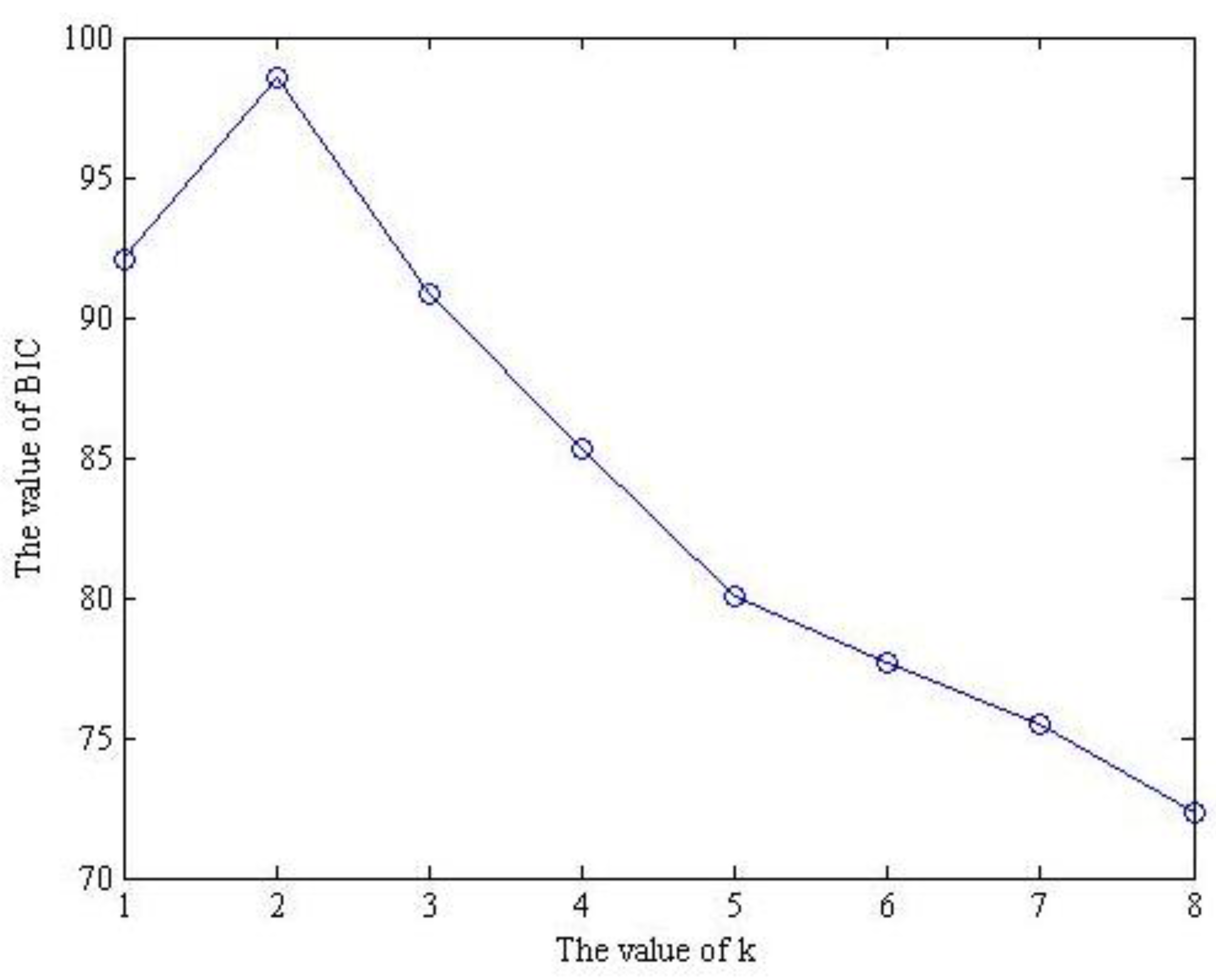
2.3. Source Number Estimation Based on Bayesian Information Criterion

Generally, BSS belongs to underdetermined blind source separation in the field of mechanical fault diagnosis. Basically, this involves the number of multi-channel observation signals being less than the number of source signals, especially in the situation of a single-channel observation signal. Since RPSEMD has the ability to adaptively decompose signals into a series of linear and stationary IMFs, it is hypothesized that the IMFs obtained from RPSEMD can solve the problem of underdetermined BSS. Nevertheless, the number of source signals of the system should be first estimated. The single channel observation signal x ( t ) is decomposed by RPSEMD to obtain sub-band components c i ( t ) ( i = 1 , 2 , ... d ) and the remainder r d ( t ) . Following this, x ( t ) and the sub-band components of the decomposition are composed of a multi-dimensional observation signal x i m f ( t ) = ( x ( t ) , c 1 ( t ) , ... , c d ( t ) , r d ( t ) ) T . In addition, the correlation matrix of x i m f ( t ) is defined as
R x = E [ x i m f ( t ) x i m f H ( t ) ]
where the operator of H is the complex conjugate transformation. When the noise belongs to Gaussian distribution and the corresponding IMFs are not relevant, the correlation matrix of x i m f ( t ) = ( x ( t ) , c 1 ( t ) , ... , c d ( t ) , r d ( t ) ) T is expressed as
R x = E [ s ( t ) s H ( t ) ] + σ 2 I v d
where v is the dimension of new observed signal x i m f ( t ) , I v d is unit matrix and σ 2 is the noise power.
Performing singular value decomposition on R x gives the following expression:
R x = V s Λ s V s T + V z Λ z V z T
where Λ s = d i a g { λ 1 , ... , λ d } are the principal eigenvalues in descending order, while Λ z = d i a g { λ d + 1 , ... , λ v } is the characteristic values for noise. Commonly, there is often clear distinction of the characteristic value between the noise components and useful signals. Therefore, for an accurate estimation of the covariance matrix and under the premise that the noise variance is relatively small, the dimensions of noise subspace of R x can be determined through judging the feature eigenvalue. Thus, the number of source signals can be obtained theoretically. However, it is difficult to determine the threshold value of the main characteristic value and the noise characteristic value. Therefore, the dimension of the noise subspace cannot be judged accurately. In order to solve the problem of threshold setting, the Bayesian information criterion (BIC) is employed to estimate the dimensions of the source signal and the noise subspace. BIC establishes the method of source number estimation based on the Bayesian Minaka selection model [41]. Thus, the BIC model can be approximately expressed as
BIC ( k ) = ( j = 1 k λ j ) N / 2 σ ~ k N ( l k ) / 2 N ( d k + k ) / 2
where σ ~ k 2 = ( j = k + 1 l λ j ) / ( l k ) , d k = l k k ( k + 1 ) / 2 , 1 k l , l is the number of non-zero eigenvalues. The goal of BIC is to find the maximum value of the cost function, which corresponds to the estimated number of source signals.

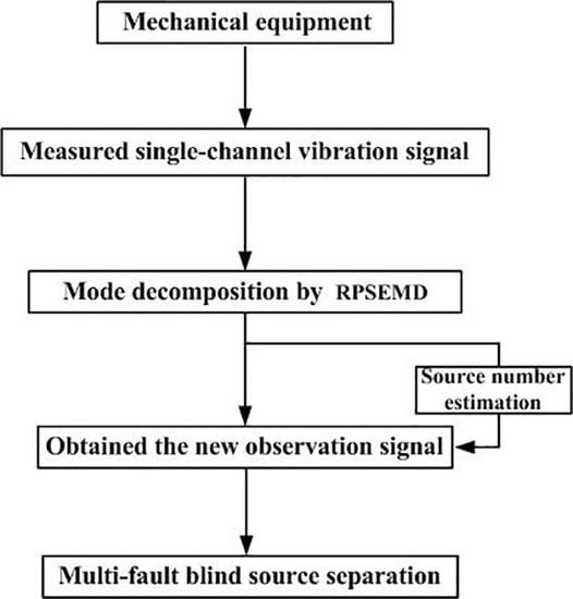
2.4. The Main Computational Steps of the Proposed Method

The main steps of the proposed BSS method for a single-channel composite signal based on RPSEMD are described as follows:
(1)
Decompose the single-channel observation signal x ( t ) by RPSEMD, with a series of linear and stationary IMFs c 1 , c 2 , ... , c n and residual component r 1 n being obtained;
(2)
The new multi-dimensional observation signal x i m f = ( x , c 1 , c 2 , ... , c n , r 1 n ) T is composed by IMFs obtained from RPSEMD and the original signal itself. In this way, the dimension of the observation signal can be increased, so that the new observation signal can be analyzed in accordance with the blind source separation theory;
(3)
Estimate the number of source signals by employing the Bayes information criteria;
(4)
According to the estimation number of the source signal, the method of feature matrix joint diagonalization based on the four-order accumulation is used to perform blind source separation on the recombination observation signal x i m f , so as to obtain the estimation s of the source signal s .

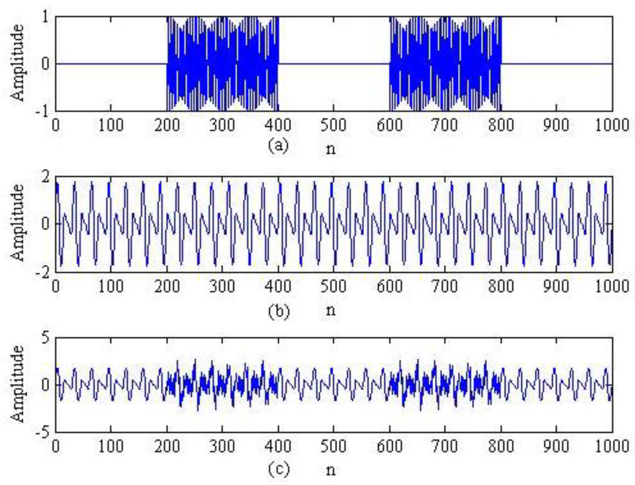
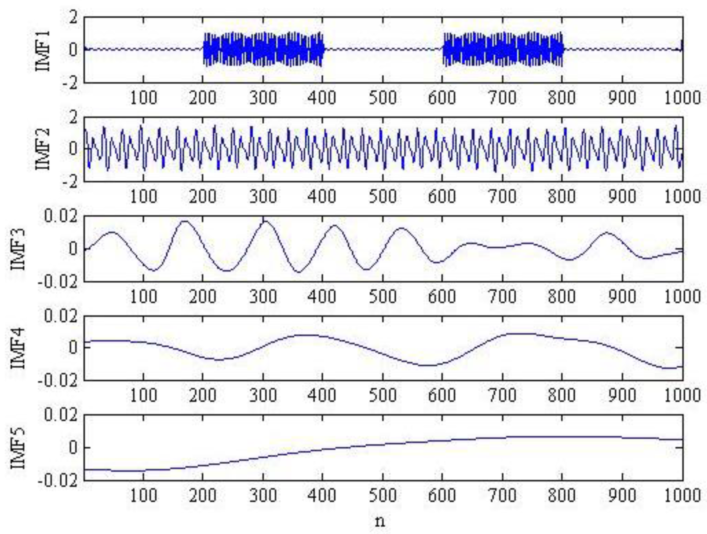
3. Simulation Signal Analysis

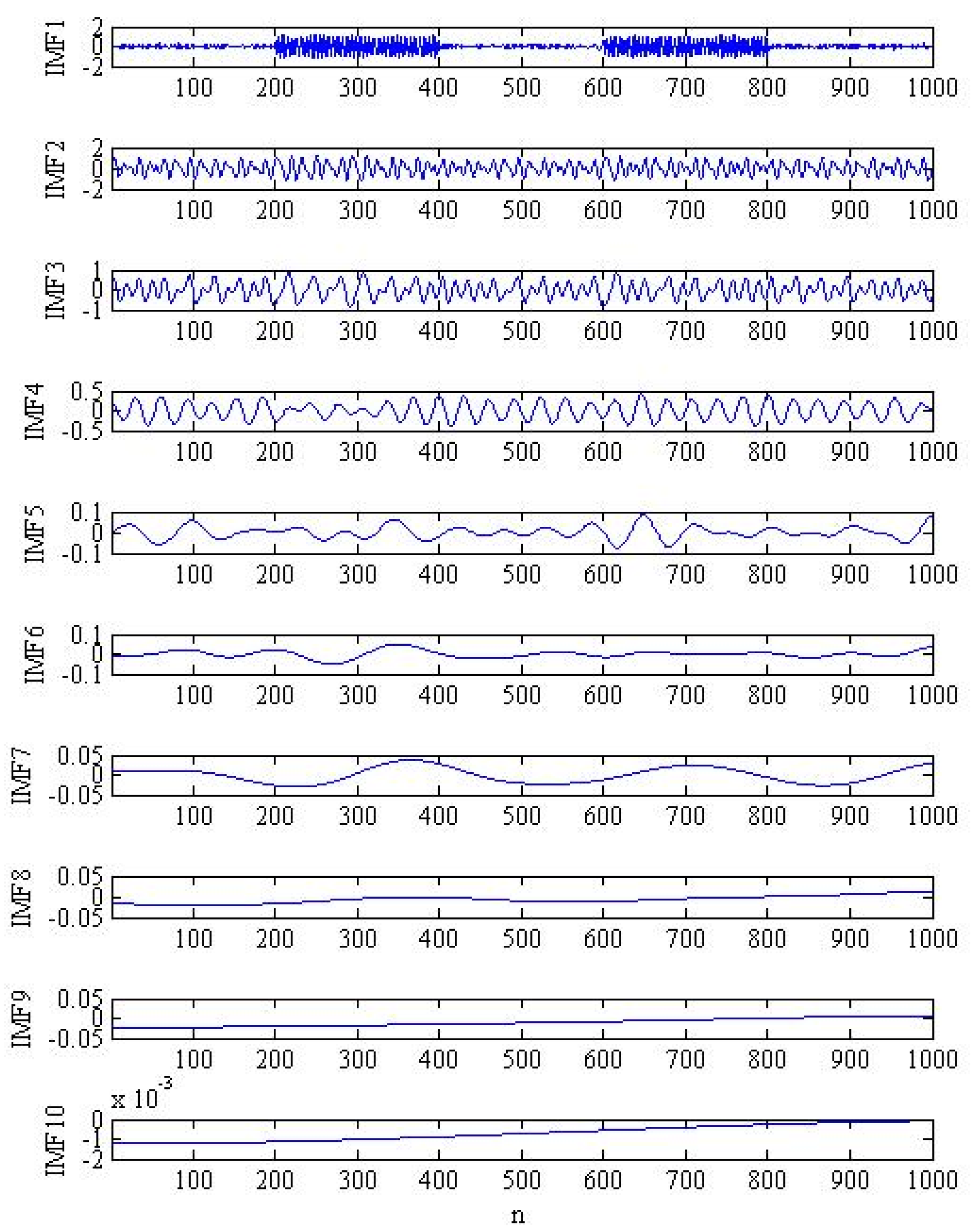
3.1. The Performance of Mode Decomposition Provided by the Proposed Method

For the first simulation, we present a classical mode mixing example here. A modulating pure signal plus an intermittent harmonic signal will inevitably lead to mode mixing when it is analyzed by EEMD, due to the local nature of the method. The analyzed signal is y = x 1 + x 2 with
x 1 = { 0 i f 1 n 200 sin ( 2 π f 1 ( n 501 ) ) i f 201 n 400 0 i f 401 n 600 sin ( 2 π f 1 ( n 501 ) ) i f 601 n 800 0 i f 801 n 1000
x 2 = sin ( 2 π f 2 n ) ( 1 + sin ( 2 π f 3 n ) )    1 n 1000
where f 1 = 0.255 , f 2 = 0.065 and f 3 = 0.032 . The mixed simulation signal is plotted in Figure 1. Table 1 shows the parameter selection for EEMD.
Moreover, the result provided by the introduced method and EEMD is drawn in Figure 2 and Figure 3, respectively.
The optimal amplitude of the noise is set as 0.2 and the ensemble size is 200 for the EEMD method. Nevertheless, parameter selection is not necessary for RPSEMD. It can be seen from Figure 2 that the IMF1 and IMF2 correspond to the original intermittent harmonic signal and modulating pure signal, respectively. However, more unreasonable mode functions have been generated in EEMD. Thus, RPSEMD outperforms EEMD in the mode decomposition of complex signal.

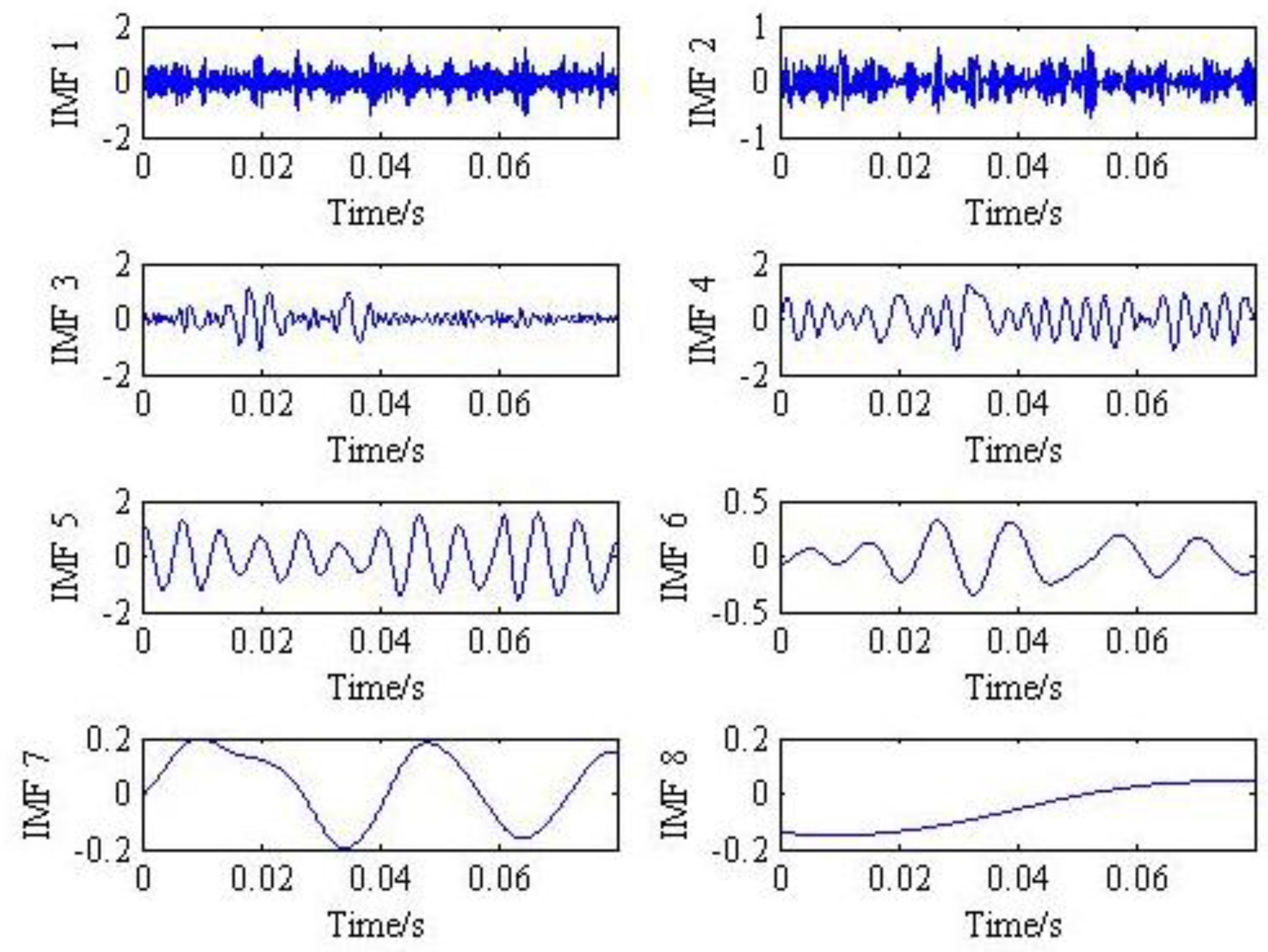
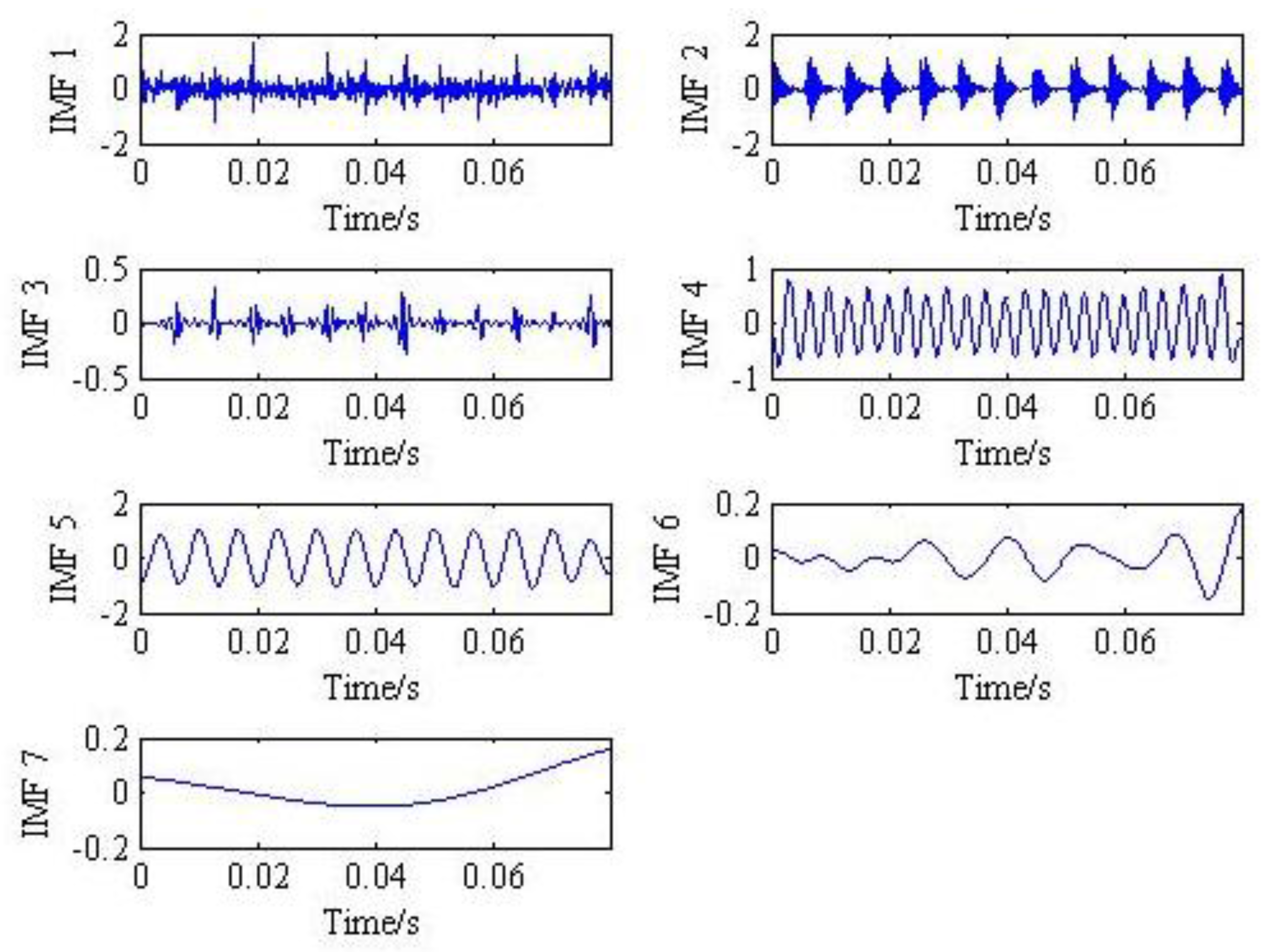
3.2. Multi-Fault Separation of Simulation Signal Analysis

Rolling-bearings and gears are always the critical components for rotating machinery. If they are under running and heavy load for a long time, they are prone to fatigue damage. Commonly, the basic fault model of a gear is described as [43]
s m ( t ) = k = 1 K A k cos ( 2 π k f m t + ϕ k )
where f m is gear-mesh frequency, k is the order of harmonic components, A k and ϕ k correspond to the amplitude and phase of the k-th harmonic respectively.
There are many types of the simulation signal models for bearing faults, with the most typical one having been proposed by Randall [44]. Thus, the simplified model of the rolling-bearing inner race fault is expressed as follows:
s b ( t ) = i = 0 M [ A 0 cos ( 2 π f r t + ϕ A ) + C A ] e B ( t i T τ i ) cos [ 2 π f n ( t i T τ i ) + ϕ w ]
where A 0 is the amplitude of resonance; f r is the rotational frequency; ϕ A , ϕ w , C A are selected as arbitrary constants; B is the attenuation coefficient; T is defined as the average time between two impacts with T = 1 / f i ; f i is the inner race fault characteristic frequency; τ i is regarded as the time lag from its mean period due to the presence of slip and f n is the resonance frequencies of the bearing system.
In order to validate the proposed method without loss of generality, the following gear fault simulation signal based on Equation (11) is studied:
s 1 = cos ( 2 π f 1 t + 25 ) + 0.55 cos ( 4 π f 1 t + 60 )
where the mesh frequency is set as f 1 = 150 Hz. Meanwhile, the inner race fault model s 2 is examined according to Equation (12), with the parameter selection being listed in Table 2. Furthermore, the noise components s 3 cannot be neglected and they can be defined as additive white Gaussian noise, whose variance is 0.5 and average is 0.
In order to randomly mix the three simulated original signals, a random 3 × 3 matrix ( A is optionally employed by the computer as
A = ( 0.9371 0.3212 0.4948 0.8352 0.0151 1.2158 1.0945 1.1645 1.5908 )
According to the instantaneous mixed signal model x ( t ) = A s ( t ) , where x = ( x 1 , x 2 , x 3 ) and s = ( s 1 , s 2 , s 3 ) , three mixed signals can be obtained.
We assumed that only a single-channel composite signal is measured, due to the limitation of monitoring conditions in the process of blind source separation of mechanical failure. Following this, the time-domain diagram of the original simulation signal s 1 , s 2 and the analyzed single-channel composite signal x 1 ( t ) are shown in Figure 4.
Figure 5 presents the IMF components obtained by RPSEMD. The IMFs provided by EEMD for the mixed fault simulation signal is plotted in Figure 6. When comparing Figure 5 and Figure 6, the RPSEMD result has better correspondence with the ideal IMFs. For instance, the IMF2 has a greater similarity with the rolling-bearing fault signal. Moreover, IMF5 and IMF4 correspond closely to the gear fault signal. However, the IMFs provided by EEMD have less relevance to the original source signal. From the graph, it can be seen that the RPSEMD has obvious advantages in the signal decomposition for the simulation signal, which can be used to identify the source signal.
After this, the single-channel observation signal x 1 ( t ) and its intrinsic mode function ( I M F 1 , I M F 2 , ... , I M F 7 ) are collected to form a new multi-dimensional signal x lim f = ( x 1 , I M F 1 , I M F 2 , ... , I M F 7 ) T , whose correlation matrix is expressed as R x = E ( x lim f ( t ) x lim f H ( t ) ) . Following this, the singular value decomposition (SVD) to the correlation matrix R x is performed, with the feature vector Λ = d i a g { λ 1 , λ 2 , ... , λ 8 } being obtained.
According to the BIC value shown in Figure 7, the number of source signals is determined as two, which is consistent with the physical truth. In addition to the original single-channel signal, it was necessary to select one component from the inherent IMFs obtained by RPSEMD, thus satisfying the basic conditions of BSS.
Since the IMF2 has the maximum correlation with the original signal, it can be chosen as the preferred mode component and is used together with the original single-channel signal to form x lim f = ( x 1 , I M F 2 ) T . It is employed as a new multi-channel observation signal to achieve the blind source separation by the approach of feature matrix joint diagonalization, based on the four-order accumulation. The results provided by the proposed method are plotted in Figure 8. When comparing Figure 4 and Figure 8, it was found that the time-domain waveform of the two components obtained by the proposed method corresponds well with the original source signals.
To verify the effectiveness of the proposed method, EEMD based on feature matrix joint diagonalization is applied to the simulation signal. Since the IMF5 generated by EEMD has the maximum correlation with the original signal, the new observed multi-channel signal is expressed as x lim f = ( x 1 , I M F 5 ) T . Following this, the result is plotted in Figure 9, which shows that the compound fault can hardly be identified. Thus, we can make a conclusion that the proposed method not only realizes the decomposition of single-channel vibration signal, but also further achieves the BSS.

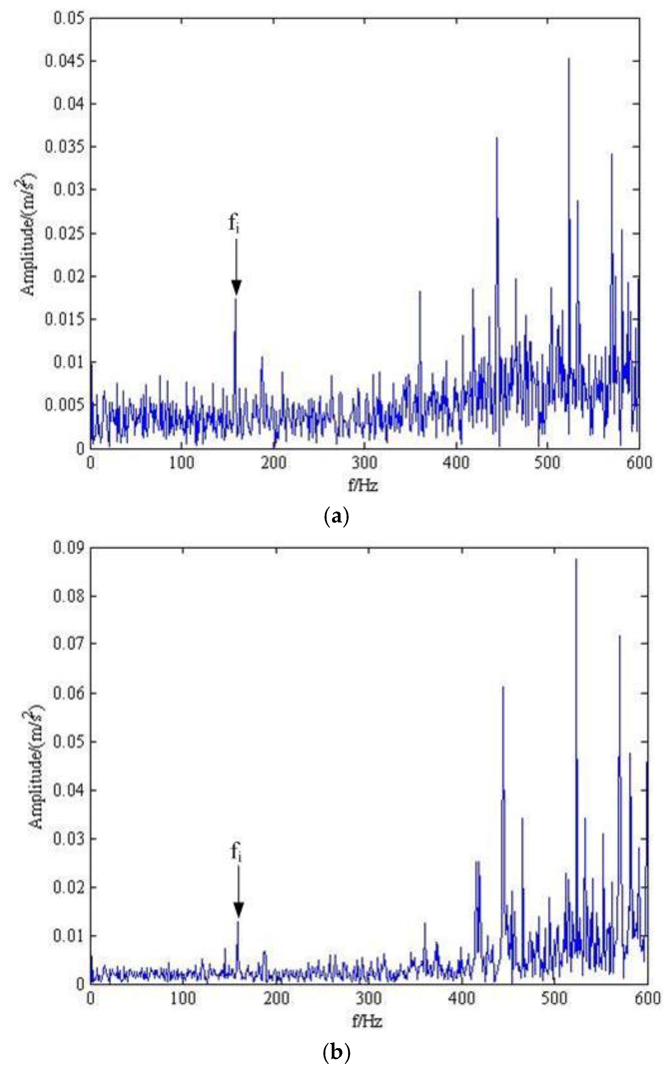
4. Analysis of the Rolling-Bearing on an Experimental Bench

Generally, the rolling-bearing is an important part of machinery. In the actual operation, the inner ring, the outer ring and rolling element parts are related to each other. Hence, there is a strong correlation between the different vibration sources. Limited by the testing experiment, one channel observation signal is monitored in normal conditions. In order to verify the validity of the proposed method in the experiment, this signal was used to detect the coupling faults of the inner and outer rings of a rolling-bearing. The experimental apparatus was provided by the experimental center of institute of mechanical automation in Wuhan University of Science and Technology, which is customized by the American SQi company. This apparatus was composed of a motor drive, encoder, and fault simulation of the two-level reduction gear box and load device. The specific device is shown in Figure 10.
In this paper, the deep-groove ball bearing ER-16k (FAFNIR, Springfield, MA, USA) with faults on the outer and inner rings was simulated. According to the bearing parameters and the coefficient of the gear transmission ratio, the frequency of the inner ring and the outer ring of the bearing fault were calculated, which are listed in Table 3.
It is noted that f is the actual motor rotational frequency, which corresponds to the input shaft frequency. Motor rotating frequency was set to be 30 Hz. As the speed of the three-phase asynchronous motor will fluctuate, the measured rotating frequency is f = 29 Hz in reality. Hence, the characteristic frequencies of the inner and outer rings of the bearing can be calculated as f i = 157.47 Hz and f o = 103.59 Hz, which are shown in Table 4. The original time-domain waveform and frequency spectrum of the measured single-channel are shown in Figure 11.
In order to perform the blind source separation of a single-channel composite signal in the experiment station, the RPSEMD was first employed to decompose the composite signal, with the mode components then being obtained. Subsequently, the original signal and the decomposed mode components were decomposed by SVD to obtain characteristic values, before the number of source signals was determined by the method of BIC. Following this, the new observation signal was processed by the proposed blind source separation and the analyzed result is drawn in Figure 12.
Figure 12a,b present the frequency spectrum of the estimated signal by the proposed method. From Figure 12a, the rotating frequency f r and its double frequency 2 f r can be inspected. In addition, the inner ring fault frequency f i , its double frequency 2 f i and its third harmonic frequency 3 f i can also be identified. Moreover, the modulation phenomenon is rather obvious, which can further prove the inner fault of roll-bearing. Analogously, the outer ring fault frequency f o , its double and triple frequencies can also be found in Figure 12b. Therefore, the method proposed in this paper can accurately identify the fault frequency of the inner ring and the outer ring, which achieves the blind source separation of a multi-fault composite signal in the experimental table.
In a similar way, the above-mentioned EEMD method for BSS [31] was compared with the proposed method, with the result being plotted in Figure 13. Nevertheless, it has little difference in the frequency domain and only the inner ring fault frequency f i can be identified. Based on Figure 12 and Figure 13, we can make the judgment that the proposed method performs better in actual, measured multi-fault signal separation.

5. Conclusions

Single-channel blind source separation algorithm (SCBSS) has important theoretical and practical values in the multi-fault feature extraction for mechanical equipment. The main work in this paper is summarized as follows: (1) A novel regenerated phase-shifted sinusoid-assisted empirical mode decomposition (RPSEMD) method was introduced for signal decomposition. It not only inhibited the mode mixing problem during the whole decomposition process, but also had superiority without parameter selection. As it produces the better performance of adaptive signal decomposition, it was first applied to the blind source separation of a single-channel composite signal in health monitoring of key mechanical equipment; (2) Based on the Bayesian information criterion and singular value characteristics generated by SVD model, the number of source signals was accurately estimated; (3) Through theoretical analysis and experimental tests, it was shown that the method proposed in this paper could effectively extract the fault features and solve the problems of multi-fault separation. Therefore, the proposed method could serve as a powerful tool in multi-fault identification.

Acknowledgments

This work was supported by the National Natural Science Foundation of China under Grants Nos. 51475339, 51405353 and 51105284; the Natural Science Foundation of Hubei province under Grant No. 2016CFA042 and the State Key Laboratory of Refractories and Metallurgy, Wuhan University of Science and Technology under Grant No. ZR201603.

Author Contributions

Cancan Yi and Yong Lv conceived and designed the experiments; Cancan Yi and Han Xiao performed the experiments; Cancan Yi and Han Xiao analyzed the data; Cancan Yi and Guanghui You contributed reagents/materials/analysis tools; Cancan Yi and Zhang Dang wrote the paper.

Conflicts of Interest

The authors declare no conflict of interest.

References

  1. Li, Y.; Xu, M.; Wang, R.; Huang, W. A fault diagnosis scheme for rolling bearing based on local mean decomposition and improved multiscale fuzzy entropy. J. Sound Vib. 2016, 360, 277–299. [Google Scholar] [CrossRef]
  2. Yi, C.; Lv, Y.; Dang, Z.; Xiao, H. A Novel Mechanical Fault Diagnosis Scheme Based on the Convex 1-D Second-Order Total Variation Denoising Algorithm. Appl. Sci. 2016, 6, 403. [Google Scholar] [CrossRef]
  3. Yi, C.; Lv, Y.; Dang, Z. A Fault Diagnosis Scheme for Rolling Bearing Based on Particle Swarm Optimization in Variational Mode Decomposition. Shock Vib. 2016, 2016, 9372691. [Google Scholar] [CrossRef]
  4. Xu, B.; Song, G.; Masri, S.F. Damage detection for a frame structure model using vibration displacement measurement. Struct. Health Monit. 2012, 11, 281–292. [Google Scholar] [CrossRef]
  5. Yao, P.; Kong, Q.; Xu, K.; Jiang, T.; Hou, L.; Song, G. Structural health monitoring of multi-spot welded joints using a lead zirconate titanate based active sensing approach. Smart Mater. Struct. 2016, 25, 015031. [Google Scholar] [CrossRef]
  6. Zhang, L.; Wang, C.; Song, G. Health Status Monitoring of Cuplock Scaffold Joint Connection Based on Wavelet Packet Analysis. Shock Vib. 2015, 2015, 695845. [Google Scholar] [CrossRef]
  7. Feng, Q.; Kong, Q.; Huo, L.; Song, G. Crack detection and leakage monitoring on reinforced concrete pipe. Smart Mater. Struct. 2015, 24, 115020. [Google Scholar] [CrossRef]
  8. Li, D.; Ho, S.C.M.; Song, G.; Ren, L.; Li, H. A review of damage detection methods for wind turbine blades. Smart Mater. Struct. 2015, 24, 033001. [Google Scholar] [CrossRef]
  9. Yi, C.; Lv, Y.; Dang, Z.; Xiao, H.; Yu, X. Quaternion singular spectrum analysis using convex optimization and its application to fault diagnosis of rolling bearing. Measurement 2017, 103, 321–332. [Google Scholar] [CrossRef]
  10. Belouchrani, A.; Abed-Meraim, K.; Cardoso, J.F.; Moulines, E. A blind source separation technique using second-order statistics. IEEE Trans. Signal Process. 1997, 45, 434–444. [Google Scholar] [CrossRef]
  11. Zhao, M.; Lin, J.; Xu, X.Q.; Li, X.J. Multi-fault detection of rolling element bearings under harsh working condition using IMF-based adaptive envelope order analysis. Sensors 2014, 14, 20320–20345. [Google Scholar] [CrossRef] [PubMed]
  12. Kouadri, A.; Baiche, K.; Zelmat, M. Blind source separation filters-based-fault detection and isolation in a three tank system. J. Appl. Stat. 2014, 41, 1799–1813. [Google Scholar] [CrossRef]
  13. Antoni, J. Blind separation of vibration components: Principles and demonstrations. Mech. Syst. Signal Process. 2005, 19, 1166–1180. [Google Scholar] [CrossRef]
  14. Gelle, G.; Colas, M.; Serviere, C. Blind source separation: A tool for rotating machine monitoring by vibrations analysis? J. Sound Vib. 2001, 248, 865–885. [Google Scholar] [CrossRef]
  15. Mowlaee, P.; Christensen, M.G.; Jensen, S.H. New results on single-channel speech separation using sinusoidal modeling. IEEE Trans. Audio Speech Lang. Process. 2011, 19, 1265–1277. [Google Scholar] [CrossRef]
  16. Gao, B.; Woo, W.L.; Dlay, S.S. Single channel source separation using EMD-subband variable regularized sparse features. IEEE Trans. Audio Speech Lang. Process. 2011, 19, 961–976. [Google Scholar] [CrossRef]
  17. Guo, Y.; Naik, G.R.; Nguyen, H. Single channel blind source separation based local mean decomposition for Biomedical applications. In Proceedings of the 2013 35th Annual International Conference of the IEEE, Osaka, Japan, 3–7 July 2013; pp. 6812–6815. [Google Scholar]
  18. Guo, Y.; Huang, S.; Li, Y.; Naik, G.R. Edge effect elimination in single-mixture blind source separation. Circuits Syst. Signal Process. 2013, 32, 2317–2334. [Google Scholar] [CrossRef]
  19. Pendharkar, G.; Naik, G.R.; Nguyen, H.T. Using blind source separation on accelerometry data to analyze and distinguish the toe walking gait from normal gait in ITW children. Biomed. Signal Process. Control 2014, 13, 41–49. [Google Scholar] [CrossRef]
  20. Davies, M.E.; James, C.J. Source separation using single channel ICA. Signal Process. 2007, 87, 1819–1832. [Google Scholar] [CrossRef]
  21. Chai, R.; Naik, G.; Nguyen, T.N.; Ling, S.; Tran, Y.; Craig, A.; Nguyen, H. Driver Fatigue Classification with Independent Component by Entropy Rate Bound Minimization Analysis in an EEG-based System. IEEE J. Biomed. Health Inform. 2016. [Google Scholar] [CrossRef] [PubMed]
  22. Wang, C.; Chen, J.; Xiao, F. Application of Empirical Model Decomposition and Independent Component Analysis to Magnetic Anomalies Separation: A Case Study for Gobi Desert Coverage in Eastern Tianshan, China. In Geostatistical and Geospatial Approaches for the Characterization of Natural Resources in the Environment; Springer International Publishing: Berlin, Germany, 2016. [Google Scholar]
  23. Naik, G.; Altimemy, A.; Nguyen, H. Transradial Amputee Gesture Classification Using an Optimal Number of sEMG Sensors: An Approach Using ICA Clustering. IEEE Trans. Neural Syst. Rehabil. Eng. 2015, 24, 1–10. [Google Scholar] [CrossRef] [PubMed]
  24. Maneshi, M.; Vahdat, S.; Gotman, J.; Grova, C. Validation of Shared and Specific Independent Component Analysis (SSICA) for Between-Group Comparisons in fMRI. Front. Neurosci. 2016, 10. [Google Scholar] [CrossRef] [PubMed]
  25. Di Persia, L.E.; Milone, D.H. Using multiple frequency bins for stabilization of FD-ICA algorithms. Signal Process. 2016, 119, 162–168. [Google Scholar] [CrossRef]
  26. Adali, T.; Calhoun, V.D. Complex ICA of brain imaging data. IEEE Signal Process. Mag. 2007, 24, 136. [Google Scholar] [CrossRef]
  27. Naik, G.R.; Kumar, D.K. Estimation of independent and dependent components of non-invasive EMG using fast ICA: Validation in recognising complex gestures. Comput. Methods Biomech. Biomed. Eng. 2011, 14, 1105–1111. [Google Scholar] [CrossRef] [PubMed]
  28. Guo, J.; Deng, Y. A Time-Frequency Algorithm for Noisy ICA. In Geo-Informatics in Resource Management and Sustainable Ecosystem; Springer: Berlin/Heidelberg, Germany, 2015; pp. 357–365. [Google Scholar]
  29. Hong, H.; Liang, M. Separation of fault features from a single-channel mechanical signal mixture using wavelet decomposition. Mech. Syst. Signal Process. 2007, 21, 2025–2040. [Google Scholar] [CrossRef]
  30. Mijović, B.; de Vos, M.; Gligorijevic, I.; Taelman, J.; Van Huffel, S. Source separation from single-channel recordings by combining empirical-mode decomposition and independent component analysis. IEEE Trans. Biomed. Eng. 2010, 57, 2188–2196. [Google Scholar] [CrossRef] [PubMed]
  31. Naik, G.R.; Selvan, S.E.; Nguyen, H.T. Single-Channel EMG Classification with Ensemble-Empirical- Mode-Decomposition-Based ICA for Diagnosing Neuromuscular Disorders. IEEE Trans. Neural Syst. Rehabil. Eng. A Publ. IEEE Eng. Med. Biol. Soc. 2016, 24, 734–743. [Google Scholar] [CrossRef] [PubMed]
  32. Zhao, X.; Li, M.; Song, G.; Xu, J. Hierarchical ensemble-based data fusion for structural health monitoring. Smart Mater. Struct. 2010, 19, 126–134. [Google Scholar] [CrossRef]
  33. Lv, Y.; Yuan, R.; Song, G. Multivariate empirical mode decomposition and its application to fault diagnosis of rolling bearing. Mech. Syst. Signal Process. 2016, 81, 219–234. [Google Scholar] [CrossRef]
  34. Sadhu, A. An Integrated Multivariate Empirical Mode Decomposition Method towards Modal Identification of Structures. Available online: http://journals.sagepub.com/doi/abs/10.1177/1077546315621207 (accessed on 7 January 2017).
  35. Wu, Z.; Huang, N.E. Ensemble empirical mode decomposition: A noise-assisted data analysis method. Adv. Adapt. Data Anal. 2009, 1, 1–41. [Google Scholar] [CrossRef]
  36. Wang, H.; Li, R.; Tang, G.; Yuan, H.F.; Zhao, Q.L.; Cao, X. A compound fault diagnosis for rolling bearings method based on blind source separation and ensemble empirical mode decomposition. PLoS ONE 2014, 9, e109166. [Google Scholar] [CrossRef] [PubMed]
  37. Guo, Y.; Huang, S.; Li, Y. Single-mixture source separation using dimensionality reduction of ensemble empirical mode decomposition and independent component analysis. Circuits Syst. Signal Process. 2012, 31, 2047–2060. [Google Scholar] [CrossRef]
  38. Yeh, J.R.; Shieh, J.S.; Huang, N.E. Complementary Ensemble Empirical Mode Decomposition: A Novel Noise Enhanced Data Analysis Method. Adv. Adapt. Data Anal. 2011, 2, 135–156. [Google Scholar] [CrossRef]
  39. Kouchaki, S.; Sanei, S.; Arbon, E.L.; Dijk, D.J. Tensor based singular spectrum analysis for automatic scoring of sleep EEG. IEEE Trans. Neural Syst. Rehabil. Eng. 2015, 23, 1–9. [Google Scholar] [CrossRef] [PubMed]
  40. Wang, C.; Kemao, Q.; Da, F. Regenerated Phase-Shifted Sinusoid-Assisted Empirical Mode Decomposition. IEEE Signal Process. Lett. 2016, 23, 556–560. [Google Scholar] [CrossRef]
  41. Huang, L.; Xiao, Y.; Liu, K.; So, H.C. Bayesian information criterion for source enumeration in large-scale adaptive antenna array. IEEE Trans. Veh. Technol. 2016, 65, 3018–3032. [Google Scholar] [CrossRef]
  42. Cardoso, J.F.; Souloumiac, A. Blind Beamforming for non-Gaussian Signals. IEE Proc. F Radar Signal Process. 1994, 140, 362–370. [Google Scholar] [CrossRef]
  43. Ypma, A. Learning Methods for Machine Vibration Analysis and Health Monitoring; TU Delft: Delft, The Netherlands, 2001. [Google Scholar]
  44. Randall, R.B.; Antoni, J.; Chobsaard, S. The relationship between spectral correlation and envelope analysis in the diagnostics of bearing faults and other cyclostationary machine signals. Mech. Syst. Signal Process. 2001, 15, 945–962. [Google Scholar] [CrossRef]
Figure 1. The simulation signal: (a) original intermittent harmonic signal; (b) modulating pure signal; (c) compound signal.
Applsci 07 00414 g001
Figure 2. The result provided by the regenerated phase-shifted sinusoid-assisted EMD (RPSEMD) method.
Applsci 07 00414 g002
Figure 3. The result provided by the EEMD method.
Applsci 07 00414 g003
Figure 4. The time domain response of s 1 , s 2 and the single channel compound signal x 1 ( t ) : (a) the time-domain of s 1 ; (b) the time-domain of s 2 and (c) the analyzed single channel signal x 1 ( t ) .
Applsci 07 00414 g004
Figure 5. The intrinsic mode functions (IMFs) provided by RPSEMD.
Applsci 07 00414 g005
Figure 6. The IMFs provided by EEMD.
Applsci 07 00414 g006
Figure 7. The Bayesian information criterion (BIC) of the composite original signal.
Applsci 07 00414 g007
Figure 8. Result of blind source separation provided by the proposed method: (a) The first component obtained by the proposed method and (b) The second component obtained by the proposed method.
Applsci 07 00414 g008
Figure 9. Results of blind source separation provided by the EEMD: (a) The first component obtained by EEMD and (b) The second component obtained by EEMD.
Applsci 07 00414 g009
Figure 10. Fault simulation experimental table for the rolling-bearing of a gear box. (a) The physical map of the test rig; (b) The structure diagram of the test rig: 1-motor, 2-encoder, 3-gearbox, 4-measured point and 5-load device.
Applsci 07 00414 g010
Figure 11. Time domain and frequency spectrum of a single channel composite signal. (a) The time response of a measured single channel vibration signal; (b) The frequency domain of measured single channel vibration signal.
Applsci 07 00414 g011
Figure 12. Result of blind source separation in the frequency domain provided by the proposed method. (a) The first component obtained by the proposed method. (b) The second component obtained by the proposed method.
Applsci 07 00414 g012
Figure 13. Result of blind source separation provided by EEMD. (a) The first component obtained by EEMD; (b) The second component obtained by EEMD.
Applsci 07 00414 g013
Table 1. The parameter settings for Ensemble Empirical Mode Decomposition (EEMD).
Noise Standard DeviationEnsemble SizeMaximum Number of Sifting Iterations
0.2200500
Table 2. The parameter selection for inner race fault simulation signal s 2 .
A 0 f r (Hz) f i (Hz) τ i f n (Hz) C A ϕ A ϕ w B
0.003291560.012000100800
Table 3. Main characteristic frequencies of the SQi simulation test table.
Rotating FrequencyTransmission FrequencyOutput FrequencyInner Ring Fault FrequencyOuter Ring Fault Frequency
f0.29f0.11f5.43f3.572f
Table 4. Characteristic frequencies of FAFNIR deep groove ball bearing.
Rotating Frequency f /HzInner Ring Fault Frequency f i /HzOuter Ring Fault Frequency f o /Hz
29157.47130.59

