FMS Scheduling under Availability Constraint with Supervisor Based on Timed Petri Nets

Abstract

This paper proposes an optimal solution to large-scale Flexible Manufacturing System (FMS) scheduling problems under availability constraints based on Timed Petri Nets ($\mathrm{TPNs}$). First a decomposition method of $\mathrm{TPNs}$ is proposed, then a mathematical model is derived based on their properties. The mathematical model is built to determine the optimal firing sequence of $\mathrm{TPN}$ transitions to minimize the total manufacturing time. The resulting firing sequence of $\mathrm{TPN}$ transitions is used to generate the manufacturing system supervisor operated by $\mathrm{TPN}$ and digital controllers. Several numerical examples and comparative studies are provided in this paper in order to prove the new approach’s efficiency.

1. Introduction

Flexible Manufacturing Systems (FMS) are widely used since they are swiftly adjustable to different production constraints, which improves their ability to cover different job types without major influence on the production plan [1,2]. Usually, FMS are subjected to failures caused by their resources’ degradation process, which has a direct impact on the production planning. To satisfy demand, an efficient production plan under the availability constraint has to be established leading to the identification of the optimal processing time or makespan [3,4]. Therefore, despite the risk of increasing deadlocks, both availability and limited resource constraints are considered when FMS scheduling is optimized.

Several methods dealing with FMS scheduling have been proposed [5,6,7,8] where the problem NP-hardness was the major challenge encountered [9]. In FMS scheduling, the most important task is to determine the sequence of production. This is related to the production supervision system for which all scheduling constraints must be considered as stated previously [10,11]. In the literature, several proposed controllers are based on Petri Net (PN) tools [12,13,14,15]. Ghaffari et al. [10] used theory of regions to synthetize the PN controller, which is a set of control places added to the initial $\mathrm{PN}$ model. Al-Ahmari et al. [16] applied Generalized Stochastic Petri Nets (GSPN) modules to derive a model for the workstation controller.

For PN analysis, several methods can be founded such as enumerative methods, which are adapted to FMS scheduling [8]. In fact, to solve the scheduling problem using enumerative methods, the reachability graph is entirely or partly explored to retrieve the optimal path [14]. Therefore, the optimal path connecting the initial and final markings corresponds to the optimal firing sequence of PN transitions. Several heuristic methods are developed in order to partly explore the reachability graph and find an optimal or suboptimal production plan. In this perspective, Lee and diCesare [17] present a Timed Petri Net ($\mathrm{TPN}$) modeling for scheduling problems and propose a heuristic algorithm A* [18,19,20] as the resolution approach. This approach is based on generating and explorating of a limited part of the reachability graph. These models were recently improved by Li et al. [21]. The authors proposed to use an algorithm for the single and multiple lot size scheduling problem and prove the solving heuristic procedure proposed by Xiong and Zhou [22].

The main inconvenience of enumerative methods is the significant number of reachable markings. Consequently, recent studies introduced new methods such as heuristic search algorithms and artificial intelligence methods in PN modeling for scheduling problems [23,24]. For instance, Chung et al. [25] introduced a genetic algorithm [26,27] to solve the sequencing problems relative to Petri net modeling. However, the latter method is limited to FMS with up to five machines. Saitou et al. [28] came up with a colored Petri net to model the resource allocation and the operation schedule of a special FMS class. The authors combined a genetic algorithm with a specific dispatching rule (the Shortest Imminent Operation time (SIO)) to get simultaneously the suboptimal resource allocation and the event-driven schedule of the colored Petri net. They were able to provide results with three different scenarios with up to ten machines.

The current study is motivated by the complexity of the enumerative methods’ increasing number leading to state explosion issues. Therefore, the main contribution of this paper is to derive a mathematical model based on $\mathrm{TPN}$ properties to efficiently solve the FMS scheduling. To achieve this, a decomposition methodology of $\mathrm{TPN}$ is proposed, where the initial model is decomposed into a set of Timed Marked Graphs ($\mathrm{TMGs}$) considered as a subclass of $\mathrm{TPN}$. Several decomposition methods for Petri net variants have been developed [29]. Nishi et al. [30,31] proposed a general $\mathrm{PN}$ decomposition method and coordination algorithm in order to optimize the conflict-free routing for an Automated Guided Vehicle (AGV). Ciardo et al. [32] introduced the concepts of near independence and near decomposition where the authors developed an approach for the solution of stochastic Petri net models. The developed approach is applied in the case of a flexible manufacturing system.

The second step of this work, a genetic algorithm, is introduced to solve the mathematical model in the case of larger-scale problems. The last part deals with the implementation of the above proposed solution in order to synthetize a supervisor, coupled with a decomposed $\mathrm{TPN}$ model.

The paper is organized as follows: Section 2 presents an overview of the timed Petri net and genetic algorithms. Section 3 illustrates the notations and terminology of the different variables used. Section 4 presents the basic assumptions where our FMS modeling is based. Section 5 derives a method to decompose the initial $\mathrm{TPN}$ into a set of Timed Marked Graphs ($\mathrm{TMGs}$). Section 6 details the proposed approaches to solve the scheduling framework under availability constraints. The supervisor synthesis method is illustrated in Section 7. Some illustrative examples and comparative studies are shown in Section 8. Finally, Section 9 is dedicated to the perspectives of this work.

2. Background

2.1. Timed Petri Net

Formally, a $\mathrm{TPN}$ [33] is a five-tuple $\left(P,T,O,W,h\left(T\right)\right)$ where:

$P=\left\{p_0,p_2,\dots ,p_{\left|P\right|}\right\}$	: is a non-empty finite set of places;
$T=\left\{t_0,t_2,\dots ,t_{\left|T\right|}\right\}$	: is a non-empty finite set of transitions;
$O\subseteq \left(P\times T\right)\cup \left(T\times P\right)$	: are the direct arcs from places to transitions $\left(P\times T\right)$ or from transitions to places $\left(T\times P\right)$;
$W:\left(P\times T\right)\cup \left(T\times P\right)\to \mathbb{N}$	: is the affectation function of weights to arcs, where $\mathbb{N}$ is the set of non-negative integers;
$h\left(t\right)\in h\left(T\right)$	: is the static time linked to $t$, $t\in T$.
$°p$ ($p^{°}$)	: designs the set of input transitions (respectively output) of place $p$;
$M$	: is a marking and the initial marking is denoted by $M_0$;
$M\left(p\right)$	: is a place marking;
$M[t>$	: indicates that transition $t$ is fired at marking $M$.

It is important to note that transition $t$ is enabled by marking $M$ only if $M\left(p\right)\ge W\left(p,t\right)$, $\forall t\in p^{°}$. An enabled transition satisfying its time condition can be fired. Furthermore, $P\cup T\ne \varnothing$ and $P\cap T=\varnothing$ where $\varnothing$ designs the empty set. In the literature, several classes could be derived from $\mathrm{TPN}$ from where the Timed Marked Graph ($\mathrm{TMG}$) is our endpoint of interest in this paper.

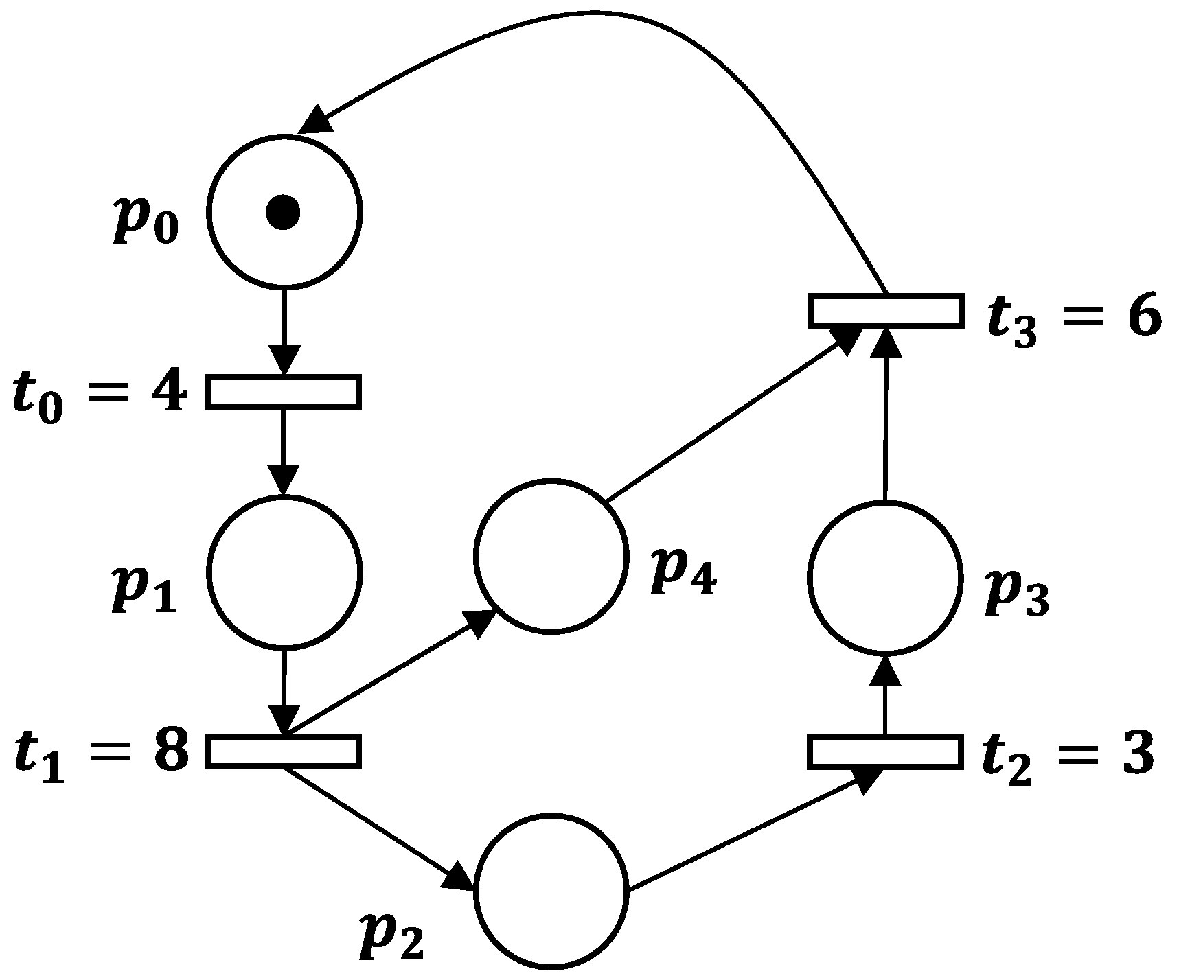
Definition 1.

The $TMG$ is a particular type of $TPN$ where every place possesses one input transition and one output transition, i.e., $\left|°p\right|=\left|p^{°}\right|=1$. Furthermore, all weights associated to arcs are equal to $one$, i.e., $W:\left(P\times T\right)\cup \left(T\times P\right)\to \left\{0,1\right\}$.

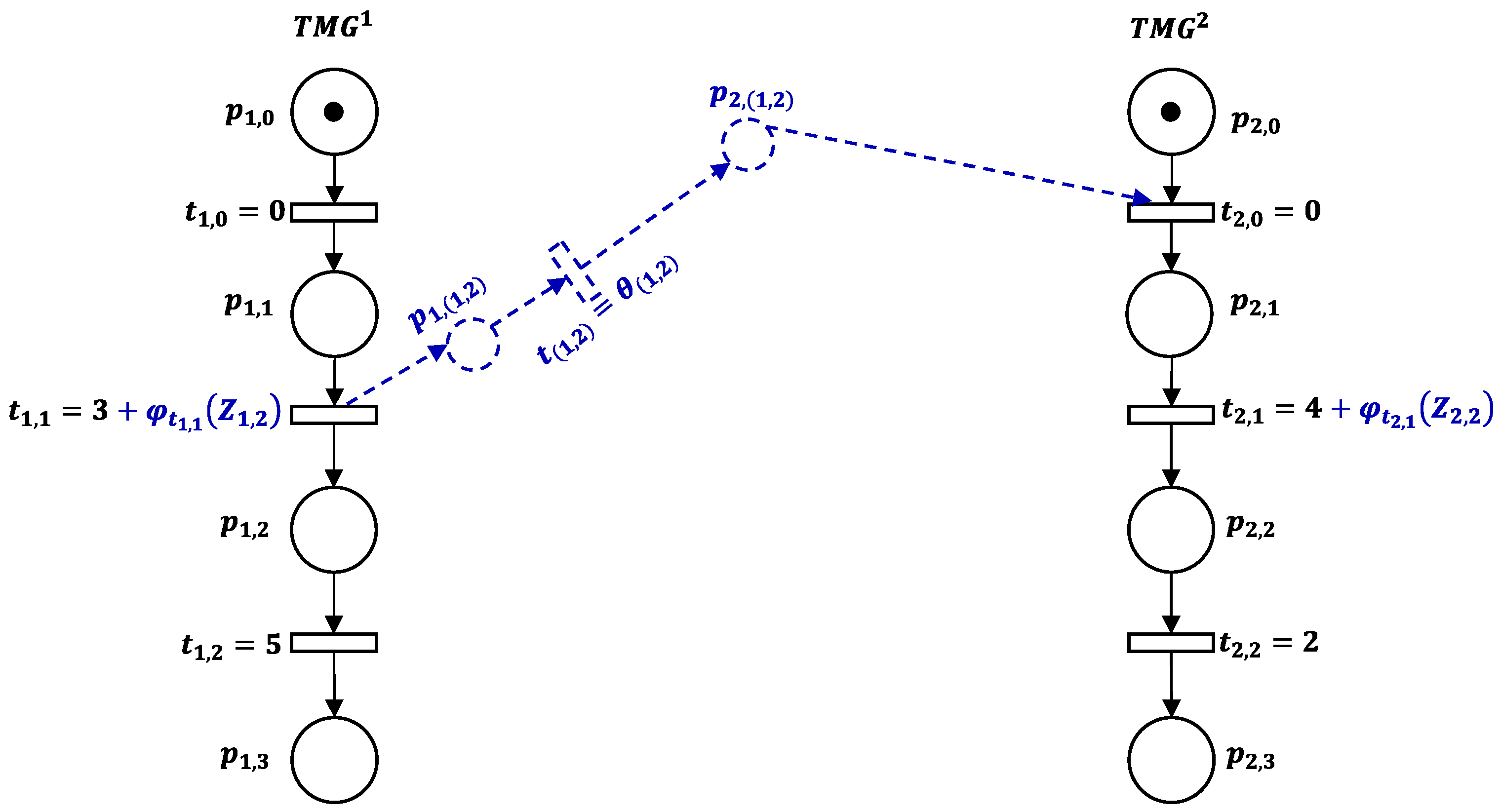
Figure 1 illustrates a $\mathrm{TMG}$ model. The place $p_0$ is initially marked, and the enabled transition $t_0$ can be fired after four time slices ($t.s$). The transition $t_1$ is fired if $p_1$ is marked with a delay of $8t.s$.

2.2. Genetic Algorithm

Genetic Algorithms ($\mathrm{GA}$) are recombination-based metaheuristics and belong to the class of evolutionary algorithms. The search procedures introduced by these algorithms are based on the mechanics of natural genetics. They have been widely applied to a variety of different problems and domains. For a detailed description of the use of genetic algorithms in engineering optimization issues, the reader could refer to Goldberg et al. [34].

In this article, we introduce the genetic algorithm method to solve the mathematical model described in the previous section. The choice of the $\mathrm{GA}$ is motivated by:

• Mathematical optimization techniques, such as the branch and bound method and dynamic programming, are limited by the problem dimensionality. These methods are not efficient in the case of large-scale and NP-hard problems, such as our study.
• The heuristic procedure is convenient for a production scheduling problem of a small scale. However, in the case of processing problems for a large scale, heuristics dealing with an NP-hard scheduling problem with a makespan objective have several drawbacks, such as the lack of comprehensiveness [35], and the accuracy of the solution needs to be improved [36].
• The genetic algorithm is convenient for production scheduling problems in view of its solving performance characteristics, such as near optimization and high resolution speed. GA efficiency was proven and discussed in solving scheduling problems having similar characteristics as our present model [37,38].

3. Terminology

In this section are presented the notations used in $\mathrm{TPN}$ modeling for FMS scheduling and supervisor synthesis.

$i,i^{*}$	: indexes for jobs ($i,i^{*}=1\dots n$);
$j,j^{*}$	: indexes for machines ($j=0\dots m+1$);
$t_{i,j}$(if fired)	: transition denoting that the job $i$ leaves the machine $j$;
$p_{i,j}$(if marked)	: place indicating that the job $i$ is already being performed by machine $j$;
$°p_{i,j}$ (${p_{i,j}}^{°}$)	: designs the set of input transitions (respectively output) of a place $p_{i,j}$;
$h\left(t_{i,j}\right)\in h\left(T\right)$	: is the local-clock linked to $t_{i,j}$; in the proposed modeling method, $h\left(t_{i,j}\right)$ defines the processing duration of $i$ through $j$;
$H\left(t_{i,j}\right)$	: is the global-clock of transition firing $t_{i,j}$; physically, it defines the end time of job $i$ through machine $j$;
$A\left(t_{i,j},t_{i^{*},j-1}\right)$	: is a decision variable defining whether the arc from $t_{i,j}$ to $t_{i^{*},j-1}$ exists;
$Z_{i,j+1}$	: is a decision variable defining whether job $i$ is performed after the maintenance task on machine $j+1$;
${\phi }_{t_{i,j}}\left(Z_{i,j+1}\right)$	: is the extra time linked to $t_{i,j}$ depending on the $Z\left(i,j+1\right)$ value;
${\pi }_{\left(t_{i,j},t_{i^{*},j-1}\right)}$	: unmarked timed elementary path between two transitions;
${\theta }_{\left(i,i^{*}\right)}$	: duration associated with ${\pi }_{\left(t_{i,j},t_{i^{*},j-1}\right)}$;
$[B_j,E_j]$	: preventive maintenance period where $B_j$ (respectively $E_j$) is the beginning time (respectively ending time).

In our proposed model for FMS using $\mathrm{TPN}$ tools (Section 5), each ${\mathrm{TMG}}^i$ designs the free-dynamics of job $i$ through the manufacturing system. Relations between two different timed marked graphs ${\mathrm{TMG}}^i$ and ${\mathrm{TMG}}^{i^{*}}$ ($i,i^{*}=1\dots n$ and $i\ne i^{*}$) are modeled by timed direct arcs $\left(t_{i,j},t_{i^{*},j-1}\right)$ from transition $t_{i,j}$ to transition $t_{i^{*},j-1}$. Physically, an established arc $\left(t_{i,j},t_{i^{*},j-1}\right)$ is interpreted to mean that the job $i$ had to be treated on machine $j$ before that the job $i^{*}$ finishes its treatment on machine $j-1$. 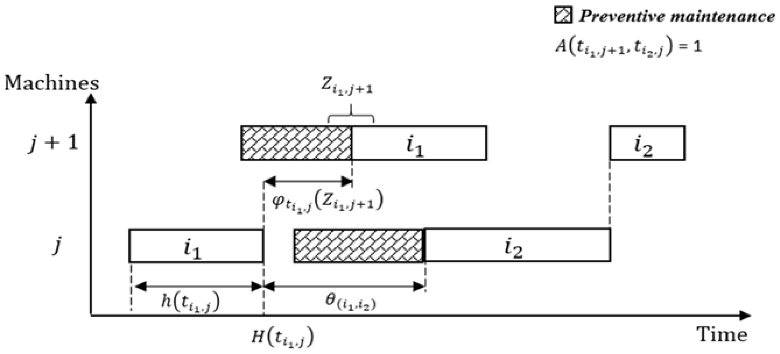$A\left(t_{i,j},t_{i^{*},j-1}\right)$ is analytically expressed as follows:

$$A\left(t_{i,j},t_{i^{*},j-1}\right)=\{\begin{array}{c}1\mathrm{if}\mathrm{the}\mathrm{timed}\mathrm{direct}\mathrm{arc}\left(t_{i,j},t_{i^{*},j-1}\right)\mathrm{has}\mathrm{taken}\mathrm{place}\\ 0\mathrm{else}\end{array}$$

(1)

Remark 1.

It is obvious that a timed direct arc between two transitions contains $\left(2\times s\right)$, $s\in \mathbb{N}$, places and $\left(2\times s-1\right)$ transitions. In the following, we consider $s=1$.

Another important parameter associated with ${\mathrm{TMG}}^i$ is the extra time ${\phi }_{t_{i,j}}\left(Z_{i,j+1}\right)\in \mathbb{N}$ added to local-clock $h\left(t_{i,j}\right)$. $Z_{i,j+1}$ corresponds to the job $i$ position, if it is just after the maintenance action on machine $j+1$. The analytical expression of $Z_{i,j+1}$ is:

$$Z_{i,j+1}=\{\begin{array}{c}1\mathrm{if}\mathrm{the}\mathrm{transition}{t}_{i,\mathrm{j}}\mathrm{should}\mathrm{not}\mathrm{be}\mathrm{fired}\\ 0\mathrm{else}\end{array}$$

(2)

Indeed, ${\phi }_{t_{i,j}}\left(Z_{i,j+1}\right)$ is the job $i$ time delay on machine $j$ until the availability of machine $j+1$. Figure 2 illustrates all of the explained parameters.

The main contribution of this paper is to carry out an efficient manufacturing supervisor based on an optimal sequence of transitions determined by a mathematical model. In this perspective, the derived supervisor is assumed to be commissioned by two types of controllers defined as follows.

TPN controller: A $\mathrm{TPN}$ controller is an unmarked timed elementary path ${\pi }_{\left(t_{i,j},t_{i^{*},j-1}\right)}:\left(p_{1,\left(i,i^{*}\right)},t_{\left(i,i^{*}\right)}\left[{\theta }_{\left(i,i^{*}\right)}\right],p_{2,\left(i,i^{*}\right)}\right)$ between two transitions $t_{i,j}$ and $t_{i^{*},j-1}$ (i.e., see Remark 1).

The principal role of the $\mathrm{TPN}$ controller is to organize the job processing via the time lag ${\theta }_{\left(i,i^{*}\right)}$. Its computing depends on the $A\left(t_{i,j},t_{i^{*},j-1}\right)$ value, where $°p_{1,\left(i,i^{*}\right)}=\left\{t_{i,j}\right\}$ and $p_{2,\left(i,i^{*}\right)}^{°}=\left\{t_{i^{*},j-1}\right\}$.

Digital controller: A digital controller model is based on the ${\phi }_{t_{i,j}}\left(Z_{i,j+1}\right)$ definition and depends on the decision variable $Z_{i,j+1}$. The role of this controller is to compute the extra time of a fully-operated job in machine $j$ when machine $j+1$ is unavailable.

4. Flexible Manufacturing System Description

This paper covers a special class of FMS, where the flexibility designs a machine that can perform different types of jobs. The time that a machine needs to change the operating mode is negligible. The considered FMS is defined as a set of multiple job types where the processing order of all jobs through the machine set is the same.

The following assumptions are considered:

• $n$ jobs of different type are initially placed in the initial buffer;
• $m$ machines are available; the initial and the final buffer will be modeled respectively by $j=0$ and $j=m+1$ as two additional virtual machines;
• Jobs are executed in the same order as defined in the first machine;
• Each machine is subject to a preventive maintenance action expressed by an unavailability period; this action is assumed to be preprogrammed;
• Each machine performs only one job at a time;
• Processing time depends on the job type;
• Job preemption is forbidden.

As mentioned, our objective is to determine the optimal sequence of jobs where the total completion time is subject to optimization. In the second part, we focus on the implementation of this optimal solution in order to synthetize the manufacturing system supervisor coupled to the initial timed Petri net.

In studies involving $\mathrm{TPN}$ models, it is often the case that there are computing risks involved, in the case of an important number of machines, so it is necessary to decompose the entire $\mathrm{TPN}$. The main objective is to guarantee an easier solving process.

5. Modeling FMS with the Decomposed TPN to the TMG Set

5.1. Decomposition Methodology

The optimal legal firing sequence problem is impossible to solve when the number of jobs and machines is increased, i.e., scalability issue. Thus, the entire $\mathrm{TPN}=\left(P,T,O,W,h\left(T\right)\right)$ explicitly models the physical functioning of FMS decomposed into several timed marked graphs, for the following reasoning. First, the set of transitions $T$ is considered as a disjoint subset $T_i$, which contains the transitions $t_{i,j}$.

$$T=T_1\cup T_2\cup \dots \cup T_n=\left(\underset{i=1}{\overset{n}{{\displaystyle \cup }}}{T}_i\right)$$

(3)

Place set $P$ presents disjoint subsets $P_i$, which contain the places $p_{i,j}$ and the set of resource-places $P_R=\left\{p_r,1\le r\le m\right\}$:

$$P=P_1\cup P_2\cup \dots \cup P_n\cup P_R=\left(\underset{i=1}{\overset{n}{{\displaystyle \cup }}}{P}_i\right){\displaystyle \cup }{P}_R$$

(4)

$$P_i=\left\{p|°p\subseteq T_{i}and{p}^{\circ }\subseteq T_i\right\}$$

(5)

Each resource-place $p_j\in P_R$ satisfies Equations (4) and (5):

$$°p_j=\left\{t_{i,j}|0\le j\le m\right\}$$

(6)

$$p_j^{\circ }=\left\{t_{i,j-1}|1\le j\le m\right\}$$

(7)

The second stage of the modeling methodology aims to remove the resource places from the entire $\mathrm{TPN}$. Indeed, the resulting $\mathrm{TPN}$ is divided into $n$ timed marked graphs ${\mathrm{TMG}}^i=\left(P_i,T_i,O_i,W_i,h\left(T_i\right)\right)$, $1\le i\le n$, which model the free-dynamic of job $i$. Hence, the place set $P_i$, direct arcs $O_i$ and affectation weights $W_i$ satisfy the following equations:

$$\underset{i=1}{\overset{n}{{\displaystyle \cup }}}{P}_i=P\backslash P_R,\forall p\in P_i$$

(8)

$$O_i\left(p,t\right)=O\left(p,t\right),\forall p\in P_i,\forall t\in T_i$$

(9)

$$O_i\left(t,p\right)=O\left(t,p\right)\forall p\in P_i,\forall t\in T_i$$

(10)

$$W_i\left(p,t\right)=0,\forall p\in P_R,\forall t\in T_i$$

(11)

$$W_i\left(t,p\right)=0,\forall p\in P_R,\forall t\in T_i$$

(12)

Therefore, ${\cup }_{i=1}^n{\mathrm{TMG}}^i$ represents the free-dynamic of jobs without considering the constraints explained in the above section. This is the reason why new parameters as timed direct arcs and extra times should be considered in the decomposed model (Section 3); parameters are computed using our methodology developed in the following section. Based on the third assumption in Section 4, the $\mathrm{TPN}$ model parameterization could be concluded through the $\mathrm{A}\left(t_{i,1},t_{i^{*},0}\right)$ value determination.

Therefore, Algorithm 1 summarizes the decomposition methodology.

Algorithm 1. The methodology of $\mathrm{TPN}$ decomposition.

Step 1. Model the considered system as a set of timed marked graphs taking into account the resource places.

Step 2. Elimination of resource places. The resulting net is ${\cup }_{i=1}^n{\mathrm{TMG}}^i$ in which each ${\mathrm{TMG}}^i$ models separately the free-dynamics of job $i$.

Step 3. Add the timed direct arcs between transitions $\left(t_{i,1},t_{j,0}\right)$, which ensure the right sequence of jobs through operators.

Step 4. Introduce the eventual extra time ${\phi }_{t_{i,j}}\left(Z_{i,j+1}\right)\in \mathbb{N}$ that presents the number of times slice delays of job $i$ in machine $j$, when the next machine $j+1$ is unavailable.

5.2. Illustrative Example

In order to illustrate the proposed $\mathrm{TPN}$ decomposition methodology, we consider an $\mathrm{FMS}$ composed of two machines $j=1,2$ operating two different jobs $i=1,2$. The processing time of jobs ($h\left(t_{i,j}\right)$) and the preventive maintenance periods ($\left[B_j,E_j\right]$) are respectively illustrated by

Table 1. The processing time.

	Machine 1	Machine 2
Part 1	3 $t.s$	5 $t.s$
Part 2	4 $t.s$	2 $t.s$

and

Table 2. The preventive maintenance periods.

	${\mathit{B}}_{\mathit{j}}$	${\mathit{E}}_{\mathit{j}}$
Machine 1	3	6
Machine 2	4	8

.

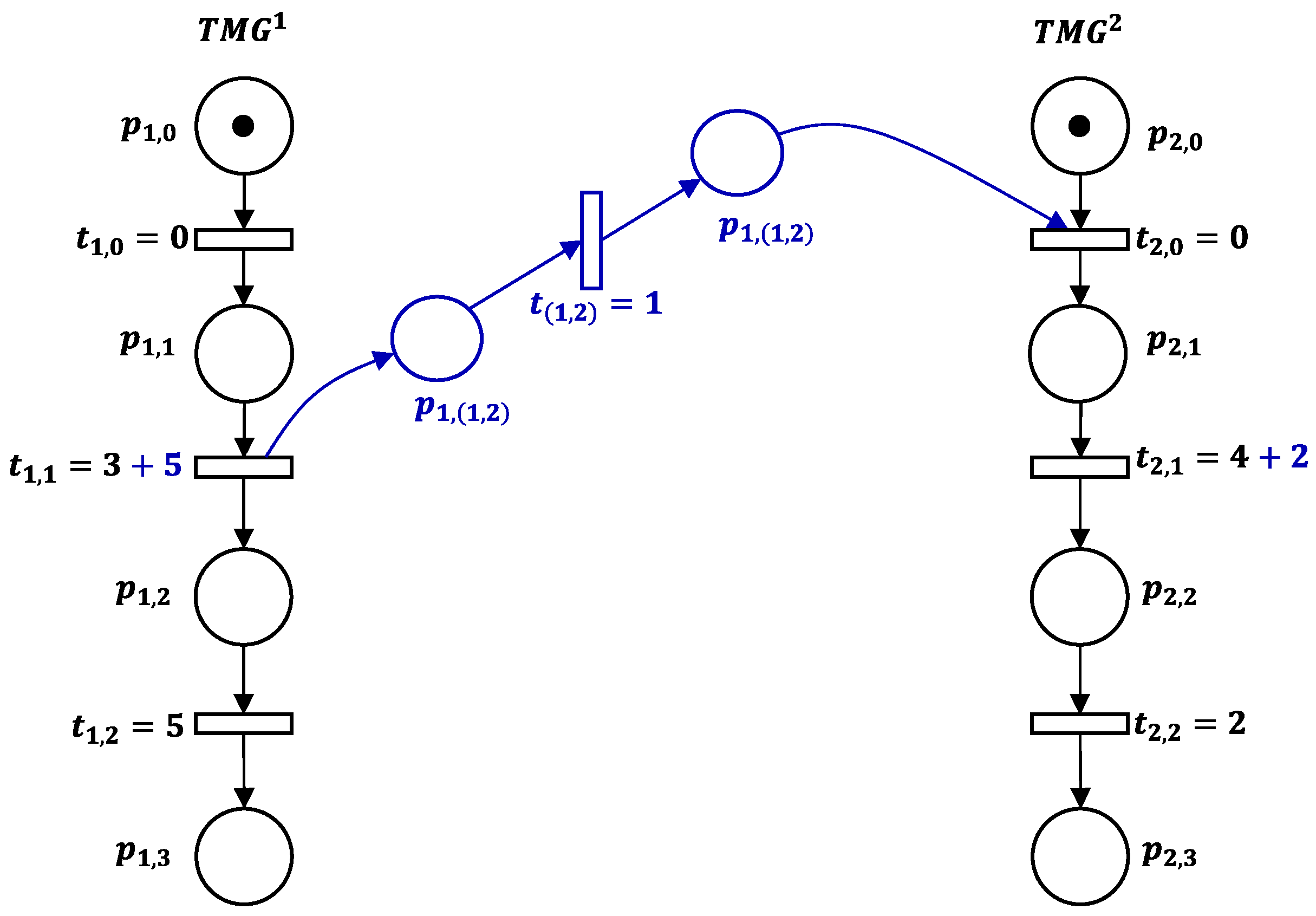
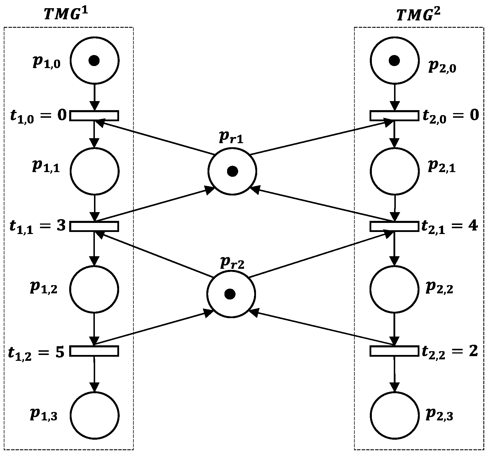
According to Figure 3, the initial timed Petri net is composed by two timed marked graphs, ${\mathrm{TMG}}^1$ and ${\mathrm{TMG}}^2$, designing respectively the free-dynamics of jobs $i_1$ and $i_2$. The initial buffer $j_0$ and the final buffer $j_3$ are considered as virtual machines. $i_1$ and $i_2$ are initially in $j_0$ corresponding with places $p_{1,0}$ and $p_{2,0}$, which are marked. Besides, the resource places $p_{r1}$ and $p_{r2}$ are designed to satisfy the production capacity constraints of $j_1$ and $j_2$. This first modeling step (Algorithm 1), satisfying Equations (12) and (13), represents the partial $\mathrm{FMS}$ scheduling with respect to the preventive maintenance and processing sequence.

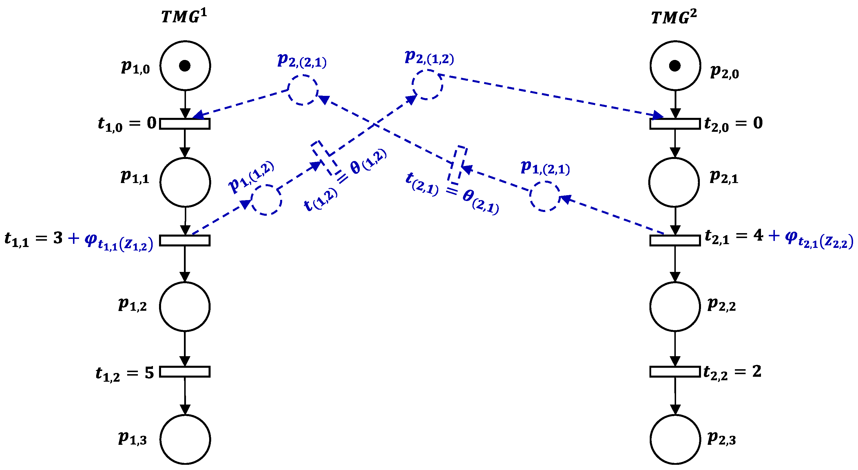
The decomposed $\mathrm{TPN}$ is determined as shown in Figure 4. It includes the direct arcs that schedule the possible processing sequences (Step 3). For instance, the timed direct arc $\left(t_{2,1},t_{1,0}\right)$ ensures the processing of $i_2$ before $i_1$ through the value of ${\theta }_{\left(2,1\right)}$. Besides, to avoid that the jobs conflict, a waiting time (Step 4) is added to corresponding transitions. For example, $\phi \left(Z\left(t_{1,c_1}\right)\right)$ represents the time delay of $i_1$ at machine $j_1$ whether $j_2$ is unavailable for maintenance.

The final scheduling through the decomposed $\mathrm{TPN}$ is determined by computing the supervisor parameters, which are the subject of the next sections.

6. Mathematical Model

A mathematical model based on decomposed $\mathrm{TPN}$ properties is proposed. The model uses the global and local clocks of transition firing (respectively $H\left(t_{i,j}\right)$ and $h\left(t_{i,j}\right)$) and the variables’ decision $A\left(t_{i,j},t_{i^{*},j-1}\right)$ and $Z_{i,j+1}$.

6.1. Model Description

A set of machines and jobs is considered. The processing duration of a job $i$ on a machine $j$ is given by $h\left(t_{i,j}\right)$. The formulation is developed to be in good agreement with the defined parameters of $\mathrm{TPN}$ modeling. In addition, a preventive maintenance scheduling constraint will be integrated to get a jointly optimal production and maintenance plan.

The objective function is defined as follows:

$$min\left(\underset{i=1..,n}{\mathit{max}}H\left(t_{i,m}\right)\right)$$

(13)

subject to:

$$H\left(t_{i,j+1}\right)-H\left(t_{i,j}\right)\ge h\left(t_{i,j+1}\right),\forall i=1,\dots n,\forall j=0,\dots m$$

(14)

$$H\left(t_{i^{*},j}\right)-H\left(t_{i,j}\right)+\alpha \cdot \left(1-A\left(t_{i,j},t_{i^{*},j-1}\right)\right)\ge h\left(t_{i^{*},j}\right),\forall i,i^{*}=1,\dots n,i\ne i^{*}\forall j=1,\dots m$$

(15)

$$H\left(t_{i,j}\right)-H\left(t_{i^{*},j}\right)+\alpha \cdot A\left(t_{i,j},t_{i^{*},j-1}\right)\ge h\left(t_{i,j}\right),\forall i,i^{*}=1,\dots n,i\ne i^{*}\forall j=1,\dots m$$

(16)

$$H\left(t_{i,j}\right)-Z_{i,j}\cdot E_j\ge h\left(t_{i,j}\right),\forall i=1,\dots ,n,\forall j=1,2,\dots ,m$$

(17)

$$H\left(t_{i,j}\right)-\alpha \cdot Z_{i,j}\le B_j,\forall i=1,\dots n,\forall j=1,2,\dots ,m$$

(18)

$$A\left(t_{i,j},t_{i^{*},j-1}\right)=A\left(t_{i,j+1},t_{i^{*},j}\right),\forall i,i^{*}=1,\dots ,n,\forall j=1,\dots ,m-1$$

(19)

$$A\left(t_{i,j},t_{i^{*},j-1}\right)=0\mathrm{or}1\forall i,i^{*}=1,\dots ,n,\forall j=1,2,\dots ,m$$

(20)

$$Z_{i,j}=0\mathrm{or}1,\forall i,i^{*}=1,\dots ,n,\forall j=1,2,\dots ,m$$

(21)

The objective function (13) aims to minimize the firing global clock of last transitions corresponding to the last machine $m$. The constraint (14) states that a job is processed, on each machine at once, without preemption. The constraints, (15) and (16) ensure that only one job can be performed on the machine at a time. In addition, the firing sequence of transitions (production sequence) has to respect the preventive maintenance period $[B_j,E_j]$ modeled with (17) and (18). Constraint (19) ensures that the order of jobs remains the same on all machines. Constraints (20) and (21) define the restrictions for the decision variables.

The linear programming (13)–(21) is a Mixed-Integer Linear Programming (MILP) because the decision variables are constrained to be binary.

Remark 2.

In the current study, the end point of interest is the determination of $A\left(t_{i,1},t_{i^{*},0}\right)$, $\left(i,i^{*}=\mathrm{1,\; ...},n\right)$; our proposed $TPN$ model assumes that the order of jobs on the machines is the same as the order defined in the first one (Section 4 assumptions).

As mentioned, our contribution is to provide the optimal firing sequence that will be used to synthetize the scheduling supervisor. Because of large-scale scheduling problems’ NP-hardness [39,40], we propose an efficient metaheuristic approach based on the genetic algorithm model.

6.2. Genetic Algorithm

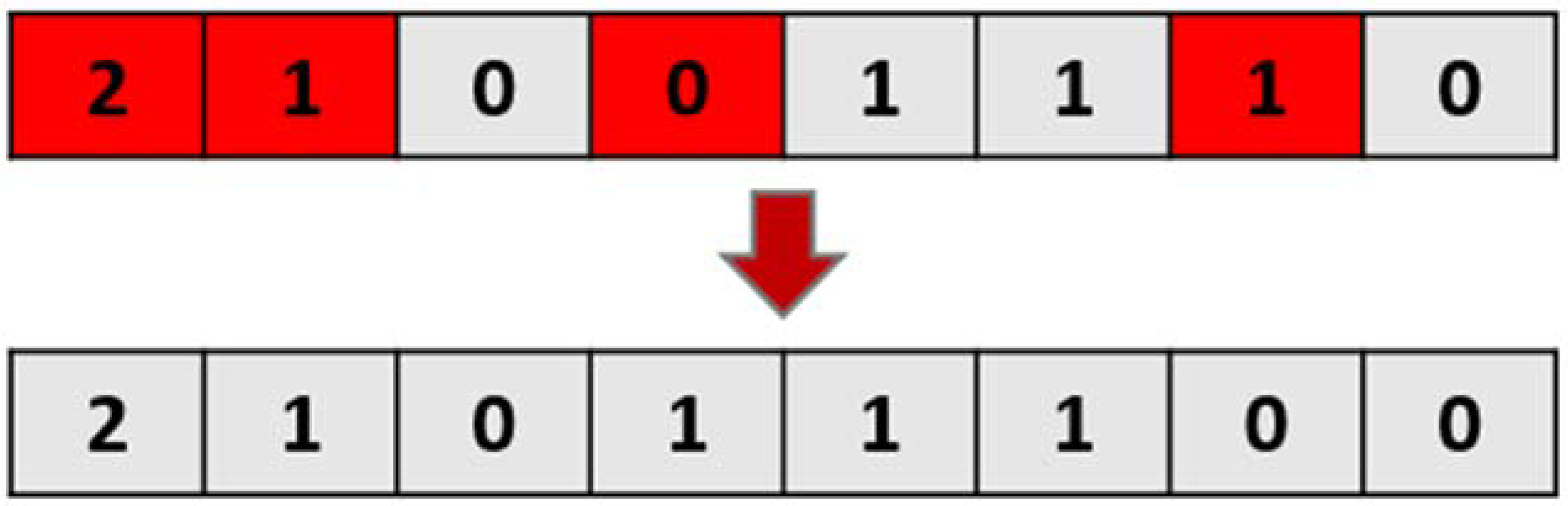
6.2.1. Encoding

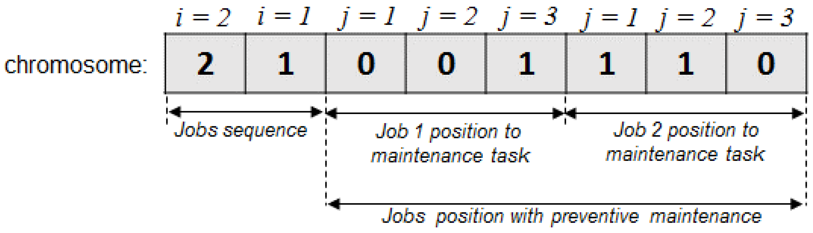
The length of the chromosome is equal to $\left(m+1\right)*n$. The first $n$ genes present the jobs’ sequence, and the last $\left(n*m\right)$ ones are binary corresponding to the job position in relation to the maintenance period on each machine (just before or after the maintenance task).

Figure 5 shows an example of the solution encoding where a set of two jobs and three machines is considered. The job number $\prime 2\prime$ will be initiated as the first job, followed by the job number $\prime 1\prime$ (two first genes). For the job number $\prime 1\prime$ (three next genes), the gene values indicate that it will be operated just before the maintenance period, in the first and the second machine, and after the maintenance period in the third one.

6.2.2. Initial Population

An initial population is generated randomly where each chromosome presents a solution for the scheduling problem.

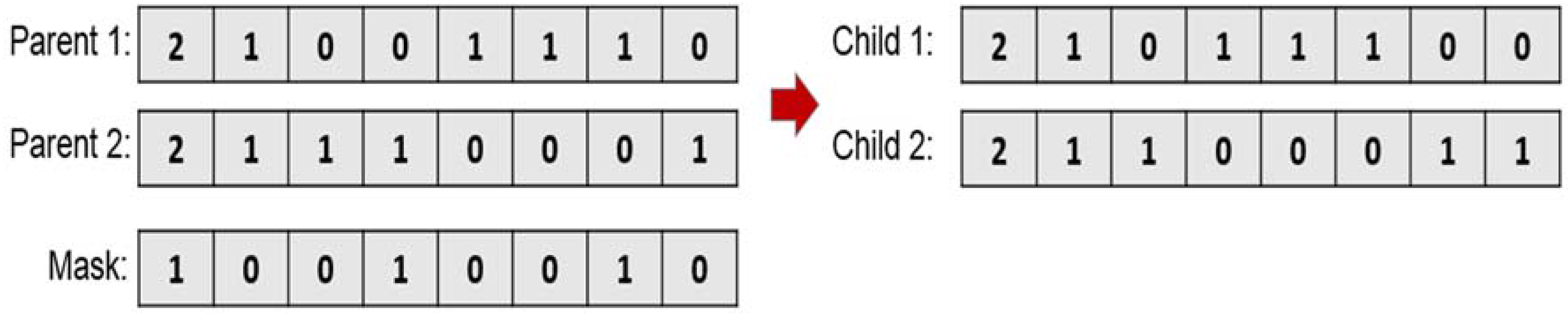
6.2.3. Crossover

There are many ways to apply the crossover operator, which aims to generate new individuals. In this perspective, a uniform crossover with a random binary mask is used. The uniform crossover uses the chromosome to switch between parent’s genes. It is possible that the crossover operator could be applied at any point (Figure 6).

6.2.4. Mutation

This operator consists of altering gene values. Figure 7 illustrates an example of the mutation mechanism application. In this example, genes subjected to mutation are Bits 1, 2, 4 and 7.

Remark 3.

Throughout the model resolution, the random gene values are selected as follows:

• For the $n$ first genes (designing jobs), the set of random bit values is $\left\{1,\dots ,n\right\}$;
• For the $\left(n*m\right)$ last genes (job position to maintenance), the set of random bit values is $\left\{1,0\right\}$.

6.2.5. Constraints

When a solution is generated, the constraints cited in Section 3 have to be respected to ensure that an individual is feasible. In addition, a test should be carried out for every new individual after we decide to reject or save it for fitness computation.

6.2.6. Fitness

The fitness function is illustrated by (13).

6.2.7. Stopping Criteria

The progress of reproduction by crossover and mutation operators and fitness continues until a satisfactory result is obtained or a preset maximum number of iterations is reached. After these iterations, the genetic algorithm prints the best chromosome that corresponds to the minimum makespan $H_{max}$.

Algorithm 2 recaps the GA steps. Initialization parameters are: population size ($P$), crossover probability value ($P_{cross}$), probability mutation value ($P_{MUT}$) and the preset maximum number of iterations ($Niter$).

Algorithm 2. Determination of the jobs’ sequence.

Initializing the program and setting the data values: $P$, $P_{cross}$, $P_{MUT}$, $Niter$, $i=0$, $k=0$

Generate randomly a solution

Repeat $i=0$

While $k<P$ do  Select randomly 2 parents of the population (2 solutions);  Apply the crossover operator;  Apply the mutation operator.  k = k + 1  End while  Test if a generated solution is feasible;  Evaluate the obtained and valid new sequences;  Arrange in ascending order these solutions based on the objective function;  Delete the worst solutions and record the best ones;  Record the best solution.  $i=i+1$  Until $i=Niter$

Print the optimal solution corresponding to minimum makespan

7. Synthesis Method of Scheduling Supervisor

The main contribution, in this part, is to develop an efficient supervisor synthesis method (Algorithm 3), which tampers with the decomposed $\mathrm{TPN}$, based on the transitions firing sequence and parameters provided by the mathematical model. The proposed supervisor is managed by two types of controllers: digital controllers and $\mathrm{TPN}$ controllers (i.e., see Section 3).

● Step 1. Solving the firing sequence:

This step is essential as it determines the firing global-clock of transitions $H\left(t_{i,j}\right)$, the decision variable values $A\left(t_{i,1},t_{i^{*},0}\right)$ and $Z_{i,j}$.

● Step 2. Identifying the chronological order of jobs:

Once $A\left(t_{i,1},t_{i^{*},0}\right)$ values are determined, one can identify the jobs’ order.

● Step 3. Deleting the inexistent direct arcs:

Direct arcs $t_{i,1},t_{i^{*},0}$ corresponding to $A\left(t_{i,1},t_{i^{*},0}\right)=0$ are removed from the decomposed $\mathrm{TPN}$ model. Remaining direct arcs ($A\left(t_{i,1},t_{i^{*},0}\right)=1$) design the selected processing sequence.

● Step 4. Determining the digital controllers:

The digital controller reacts when the treatment of job $i$ is accomplished through machine $j$ while $j+1$ is unavailable. Therefore, the controller functioning is displayed through $Z_{i,j+1}=1$ in which the extra time ${\phi }_{t_{i,j}}\left(Z_{i,j+1}\right)$ of this controller is computed.

● Step 5. Determining the $\mathrm{TPN}$ controllers:

The $\mathrm{TPN}$ controller ship is to ensure a correct order progression of jobs including among each other a time lag ${\theta }_{\left(i,i^{\prime }\right)}$. The $\mathrm{TPN}$ controllers operate in coordination with digital controllers, i.e., the determination of time lag ${\theta }_{\left(i,i^{\prime }\right)}$ takes into account the extra time ${\phi }_{t_{i,j}}\left(Z_{i,j+1}\right)$ of the digital controller. Its value is computed as: ${\theta }_{\left(i,i^{\prime }\right)}=H\left(t_{i^{\prime },0}\right)-\left(H\left(t_{i,1}\right)+\phi \left(Z\left(t_{i,1}\right)\right)\right)$.

● Step 6. Implementing the supervisor:

The controllers calculated in Steps 4 and 5 take places in the decomposed timed Petri net.

Algorithm 3. Supervisor synthesis based on the generated firing sequence.

1.  Solve the firing sequence using the mathematical model (13)–(21) and genetic algorithm. 2.  Identify the chronological order of jobs. 3.  Delete the inexistent direct arcs  For each $A\left(t_{i,1},t_{i^{*},0}\right)=0\forall i,i^{*}=1,2,\dots ,n$, $i\ne i^{*}$   Remove the direct arc $\left({\mathrm{t}}_{\mathrm{i},1},{\mathrm{t}}_{{\mathrm{i}}^{*},0}\right)$ from the decomposed $\mathrm{TPN}$ 4.  Determine the digital controllers  For each $Z_{i,j+1}=1\forall j=1,\dots ,m-2$   Calculate ${\phi }_{t_{i,j}}\left(Z_{i,j+1}\right)=H\left(t_{i,j+1}\right)-\left(H\left(t_{i,j}\right)+h\left(t_{i,j+1}\right)\right)$   For each job $s\succ i$    Calculate ${\phi }_{t_{s,j}}\left(Z_{i,j+1}\right)=H\left(t_{s,j+1}\right)-\left(H\left(t_{s,j}\right)+h\left(t_{s,j+1}\right)\right)$ 5.  Determine the $\mathrm{TPN}$ controllers  For each $A\left(t_{i,1},t_{i^{*},0}\right)=1\forall i,i\prime =1,2,\dots ,n$, $i\ne i^{*}$   Create the $\mathrm{TPN}$ controller: ${\pi }_{\left(t_{i,1},t_{i^{*},0}\right)}:\left(p_{1,\left(i,i^{*}\right)},t_{\left(i,i^{*}\right)}\left[{\theta }_{\left(i,i^{*}\right)}\right],p_{2,\left(i,i^{*}\right)}\right)$.   Calculate ${\theta }_{\left(i,i^{*}\right)}=H\left(t_{i^{*},0}\right)-\left(H\left(t_{i,1}\right)+\phi \left(Z\left(t_{i,1}\right)\right)\right)$. 6.  Implement the supervisor to decomposed $\mathrm{TPN}$

To solve the mathematical model (13)–(21), we used the Xpress optimizer. Xpress is a mathematical programming solver dealing with linear and quadratic problems in continuous and integer variables. For solving Mixed Integer Programs (MIPs), the optimizer provides a powerful branch and bound framework. The Xpress optimizer essentials, components and interfaces are found in many guides and reference manuals, from which we cite [41]. In the literature, many proposals deal with Xpress solver. Guéret [40] illustrates some applications of the optimization solver programs. Algorithms for solving large linear optimization problems are reviewed. Laundy et al. [42] highlights the Xpress solver’s efficiency to optimize mixed linear problems.

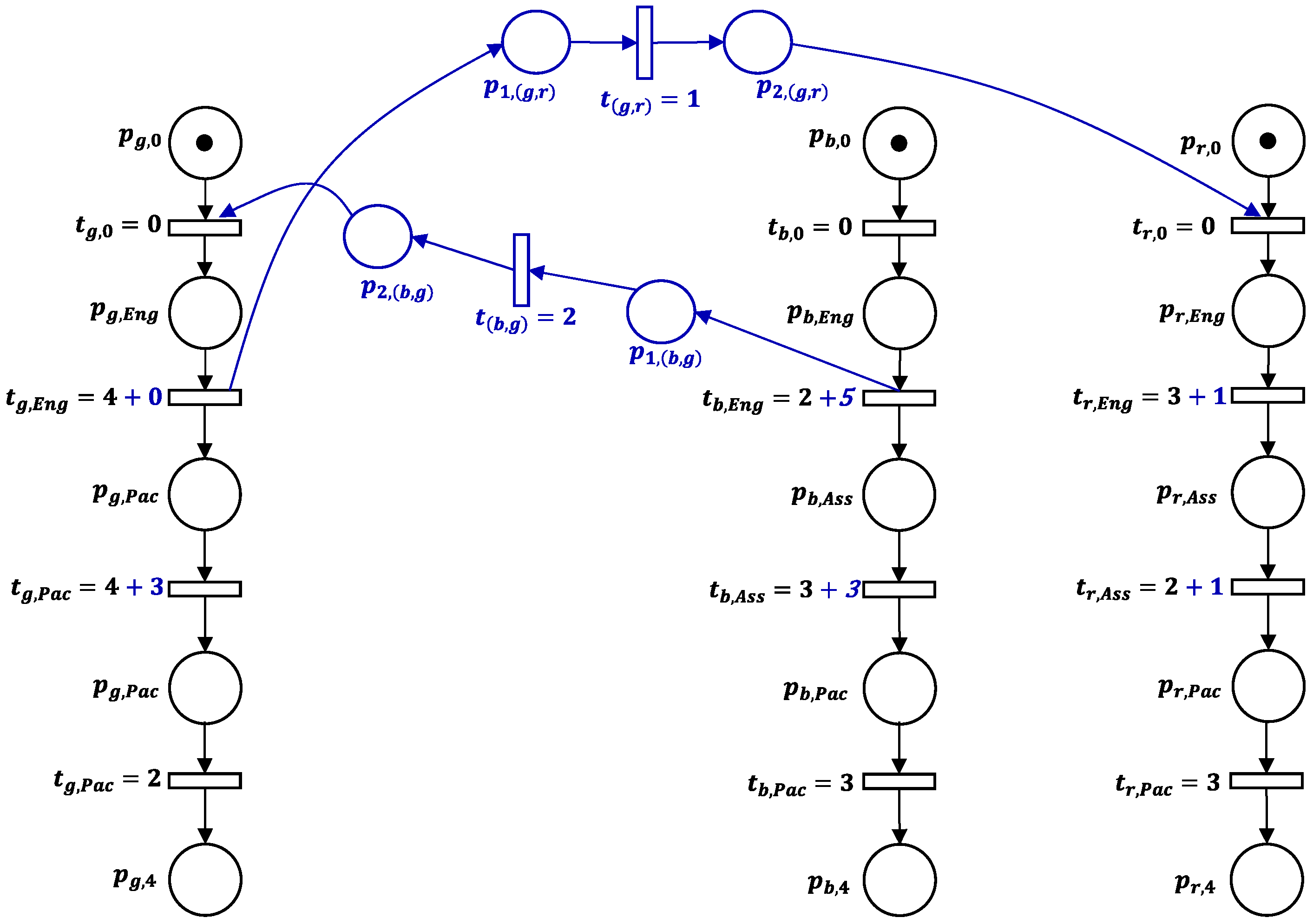
To illustrate the supervisor synthesis, we reconsider the decomposed timed Petri net shown in Figure 3 and the preventive maintenance presented in Table 2. The obtained results are shown in

Table 3. The optimal solution and decision variables.

$H\left(t_{1,0}\right)=0$	$H\left(t_{1,1}\right)=3$	$H\left(t_{1,2}\right)=13$	$H\left(t_{2,0}\right)=7$	$H\left(t_{2,1}\right)=11$
$H\left(t_{2,2}\right)=15$	$A\left(t_{1,1},t_{2,0}\right)=1$	$A\left(t_{2,1},t_{1,0}\right)=0$	$Z_{1,1}=0$	$Z_{1,2}=1$
$Z_{2,1}=1$	$Z_{2,2}=0$

.

Moreover, as explained in Step 2 of Algorithm 3, the decision variable $A\left(t_{1,1},t_{2,0}\right)=1$ expresses that the job $i_1$ is treated before the job $i_2$, ($i_1\prec i_2$). Hence, the timed direct arc $\left(t_{2,1},t_{1,0}\right)$ is removed from the decomposed $\mathrm{TPN}$, i.e., $A\left(t_{2,1},t_{1,0}\right)=0$ (Figure 8).

According to Step 3, the determination of digital controllers is related to $Z_{1,2}=1$, as follows:

$$⟹\{\begin{array}{c}{\phi }_{t_{1,1}}\left(Z_{1,2}\right)=H\left(t_{1,2}\right)-\left(H\left(t_{1,1}\right)+h\left(t_{1,2}\right)\right)=5t.s\\ As\left(i_2\succ i_1\right)⟹{\phi }_{t_{2,1}}\left(Z_{1,2}\right)=H\left(t_{2,2}\right)-\left(H\left(t_{2,1}\right)+h\left(t_{2,2}\right)\right)=2t.s.\end{array}$$

Indeed, the two digital controllers ${\phi }_{t_{1,1}}\left(Z_{1,2}\right)$ and ${\phi }_{t_{2,1}}\left(Z_{1,2}\right)$ require a waiting time respectively for $i_1$ and $i_2$ at $j_1$. Jobs $i_1$ and $i_2$ are respectively delayed by $5t.s$ and $3t.s$.

Afterward, the $\mathrm{TPN}$ controller ${\pi }_{\left(t_{1,1},t_{2,0}\right)}:\left(p_{1,\left(1,2\right)},t_{\left(1,2\right)}\left[{\theta }_{\left(1,2\right)}\right],p_{2,\left(1,2\right)}\right)$ permits a good sequence between $i_1$ and $i_2$. Its time lag ${\theta }_{\left(1,2\right)}$ is determined as follows:

➢

$A\left(t_{1,1},t_{2,0}\right)=1$

$$⟹{\theta }_{\left(1,2\right)}=H\left(t_{2,0}\right)-\left(H\left(t_{1,1}\right)+\phi \left(Z\left(t_{1,1}\right)\right)\right)=1t.s$$

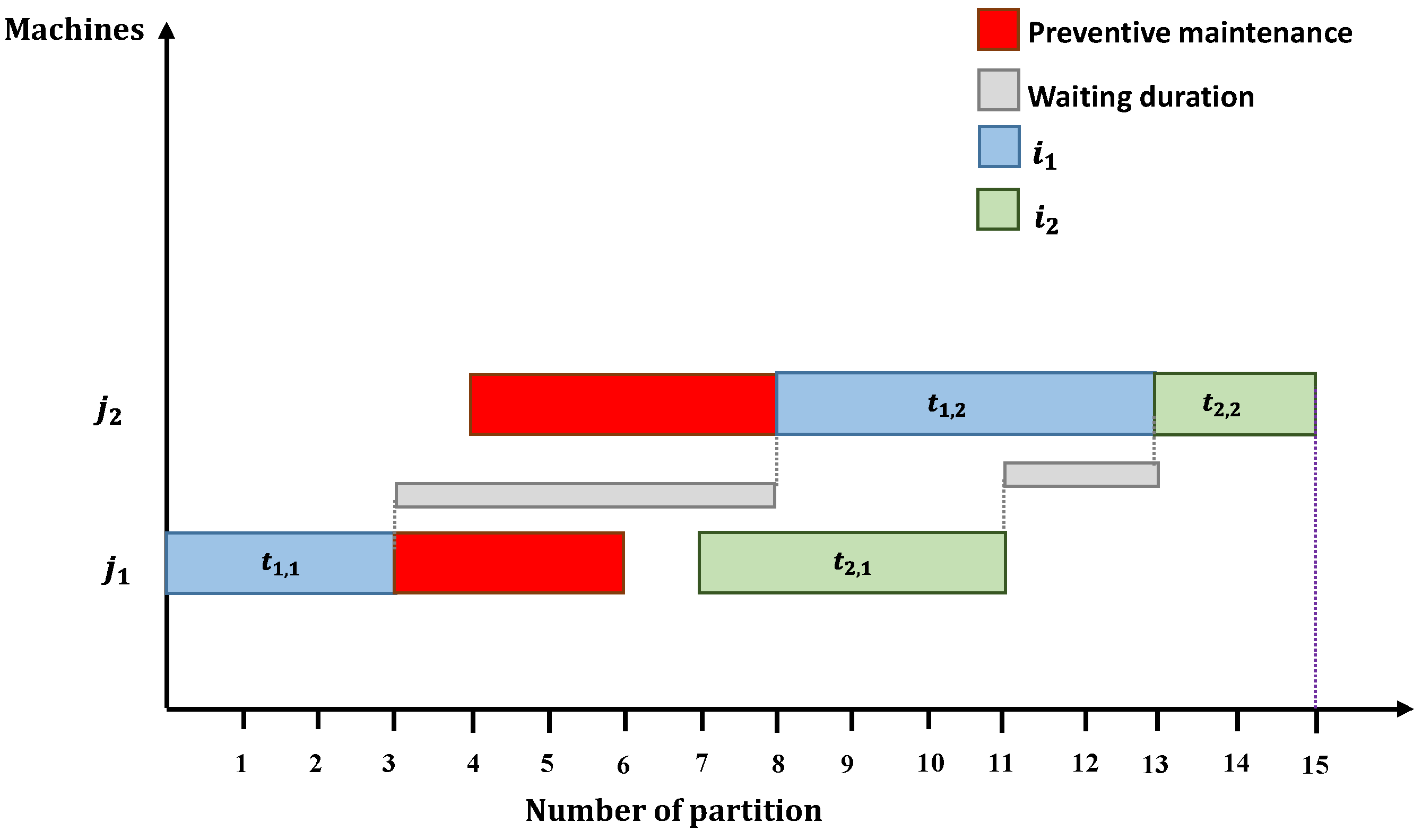
Finally, the decomposed $\mathrm{TPN}$ coupled with the synthetized supervisor, shown in Figure 9, guarantees the optimal manufacturing scheduling; i.e., the optimal sequence firing of transitions is $\sigma =t_{1,0}{t}_{1,1}{t}_{2,0}{t}_{2,1}{t}_{1,2}{t}_{2,2}$.

Figure 10 illustrates the optimal manufacturing scheduling obtained from the controlled $\mathrm{TPN}$ model.

8. Numerical Examples

A fully-automated flexible manufacturing system based at the Engineers’ National School of Metz represents the application object of our proposed approaches.

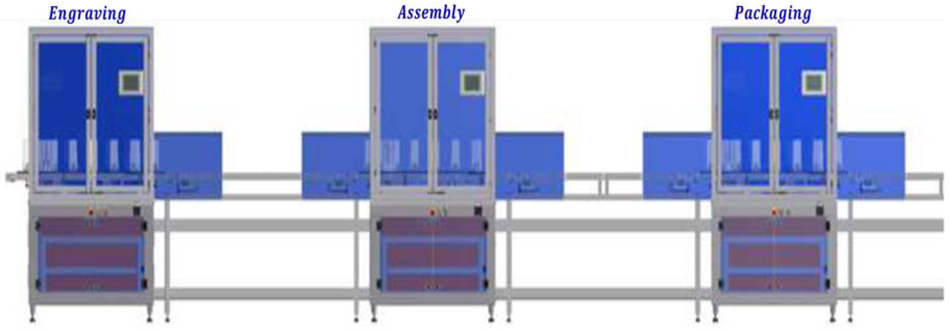
8.1. System Description

The manufacturing system consists of three machines, an initial buffer and a final buffer, which are arranged in series around a central conveyor (Figure 11). Thereby, every machine is designed to realize an operation on a glass part. Each machine function is described as follows:

$j_0$	: initial buffer;
$j_{Eng}$	: engraving of glass part by the laser;
$j_{Ass}$	: assembly of glass part engraved at a stand;
$j_{Pac}$	: packaging of the glass part engraved and assembled in a case;
$j_4$	: final buffer.

We consider that the system produces three jobs (glass parts), which are differentiated by their color: blue ($i_b$), red ($i_r$) and green ($i_g$). The processing time of every job is presented in

Table 4. Operating time.

	${\mathit{j}}_{\mathit{E}\mathit{n}\mathit{g}}$	${\mathit{j}}_{\mathit{A}\mathit{s}\mathit{s}}$	${\mathit{j}}_{\mathit{P}\mathit{a}\mathit{c}}$
Red glass part	$3$	$2$	$3$
Blue glass part	$2$	$3$	$3$
Green glass part	$4$	$4$	$2$

.

The maintenance action periods for three machines are illustrated by

Table 5. The preventive maintenance periods.

	${\mathit{B}}_{\mathit{j}}$	${\mathit{E}}_{\mathit{j}}$
${\mathit{j}}_{\mathit{E}\mathit{n}\mathit{g}}$	$2$	$7$
${\mathit{j}}_{\mathit{A}\mathit{s}\mathit{s}}$	$0$	$6$
${\mathit{j}}_{\mathit{P}\mathit{a}\mathit{c}}$	$10$	$13$

.

8.2. Illustrative Example for the Genetic Algorithm

In view of the problem NP-hardness, in the case of more than two machines apart from the initial and final buffer since they do not increase the complexity of the problem (their operating time is zero), we have proposed Algorithm 2 to solve the (13)–(21) model.

We consider the database given by Table 4 and Table 5. The genetic algorithm parameters are used as follows:

• $P=100\mathrm{individuals}$;
• $P_{cross\prime }=0.95$;
• $P_{MUT}=0.05$;
• $Niter=200$

Table 6. The optimal solution of three jobs and three machines.

The Optimal Firing Sequence
$\sigma =t_{b,0}{t}_{b,Eng}{t}_{b,Ass}{t}_{g,Eng}{t}_{b,Pac}{t}_{g,Ass}{t}_{r,Eng}{t}_{g,Pac}{t}_{r,Ass}{t}_{r,Pac}$
The resulting decision variables values
$H\left(t_{b,0}\right)=0$; $H\left(t_{b,Eng}\right)=7$; $H\left(t_{b,Ass}\right)=13$; $H\left(t_{g,0}\right)=9$; $H\left(t_{g,Eng}\right)=13$; $H\left(t_{b,Pac}\right)=16$; $H\left(t_{g,Ass}\right)=18$; $H\left(t_{r,0}\right)=14$; $H\left(t_{r,Eng}\right)=18$; $H\left(t_{g,Pac}\right)=20$; $H\left(t_{r,Ass}\right)=21H_{max}=H\left(t_{r,Pac}\right)=24$; $A\left(t_{b,Eng},t_{g,0}\right)=1$; $A\left(t_{g,Eng},t_{r,0}\right)=1$; $Z_{b,Ass}=1$; $Z_{g,Eng}=1$; $Z_{b,Pac}=1$.

illustrates the sub-optimal value for decision variables and firing sequence.

In the same way as the previous described example, the computational results (Table 3) are used to determine supervisor parameters as shown in Figure 12.

Table 7. Genetic algorithm results.

	$2$ $\left(\mathit{b},\mathit{g}\right)$	$3$ $\left(\mathit{b},\mathit{g},\mathit{r}\right)$	$4$ $\left({\mathit{b}}^1,{\mathit{b}}^2,\mathit{g},\mathit{r}\right)$	$5\left({\mathit{b}}^1,{\mathit{b}}^2,{\mathit{g}}^1,{\mathit{g}}^2,\mathit{r}\right)$
$\mathbf{2}$ $\left({\mathit{j}}_{\mathit{E}\mathit{n}\mathit{g}},{\mathit{j}}_{\mathit{A}\mathit{s}\mathit{s}}\right)$	$H\left(t_{g,Ass}\right)=18$ $A\left(t_{b,Eng},t_{g,0}\right)=1$ $Z_{b,Ass}=1$ $Z_{g,Eng}=1$	$H\left(t_{r,Ass}\right)=19$ $A\left(t_{b,Eng},t_{r,0}\right)=1$ $A\left(t_{r,Eng},t_{b,0}\right)=1$ $Z_{b,Ass}=1$ $Z_{r,Eng}=1$	$H\left(t_{r,Ass}\right)=25$ $A\left(t_{b^2,Eng},t_{r,0}\right)=1$ $A\left(t_{r,Eng},t_{g,0}\right)=1$ $A\left(t_{g,Eng},t_{b^1,0}\right)=1$ $Z\left(t_{b^2,Ass}\right)=1$ $Z_{r,Eng}=1$	$H\left(t_{g^1,Ass}\right)=33$ $A\left(t_{b^1,Eng},t_{g^2,0}\right)=1$ $A\left(t_{g^2,Eng},t_{b^2,0}\right)=1$ $A\left(t_{b^2,Eng},t_{r,0}\right)=1$ $A\left(t_{r,Eng},t_{g^1,0}\right)=1$ $Z_{b^1,Ass}=1$, $Z_{g^2,Eng}=1$
$\mathbf{3}$ $\left({\mathit{j}}_{\mathit{E}\mathit{n}\mathit{g}},{\mathit{j}}_{\mathit{A}\mathit{s}\mathit{s}},{\mathit{j}}_{\mathit{P}\mathit{a}\mathit{c}}\right)$	$H\left(t_{g,Pac}\right)=22$ $A\left(t_{b,Eng},t_{g,0}\right)=1$ $Z_{b,Ass}=1$ $Z_{g,Eng}=1$	$H\left(t_{r,Pac}\right)=24$ $A\left(t_{b,Eng},t_{g,0}\right)=1$ $A\left(t_{g,Eng},t_{r,0}\right)=1$ $Z_{b,Ass}=1$ $Z_{g,Eng}=1$ $Z_{b,Pac}=1$	$H\left(t_{b^2,Pac}\right)=30$ $A\left(t_{b^1,Eng},t_{r,0}\right)=1$ $A\left(t_{r,Eng},t_{g,0}\right)=1$ $A\left(t_{g,Eng},t_{b^2,0}\right)=1$ $Z_{b^1,Ass}=1$ $Z_{r,Eng}=1$ $Z_{b^1,Pac}=1$	$H\left(t_{r,Ass}\right)=48$ $A\left(t_{b^1,Eng},t_{g^1,0}\right)=1$ $A\left(t_{g^1,Eng},t_{b^2,0}\right)=1$ $A\left(t_{b^2,Eng},t_{r,0}\right)=1$ $A\left(t_{r,Eng},t_{g^2,0}\right)=1$ $Z_{b^1,Ass}=1$, $Z_{b^1,Pac}=1$ $Z\left(t_{g,Eng}\right)=1$

illustrates decision variables resulting from the Algorithm 2 resolution for a set of different jobs and machines. In the fourth and fifth column, we have considered new jobs: $i_{b^1}$ and $i_{b^2}$, having the same operating time as blue glass $i_b$, $i_{g^1}$ and $i_{g^2}$ as green glass $i_g$.

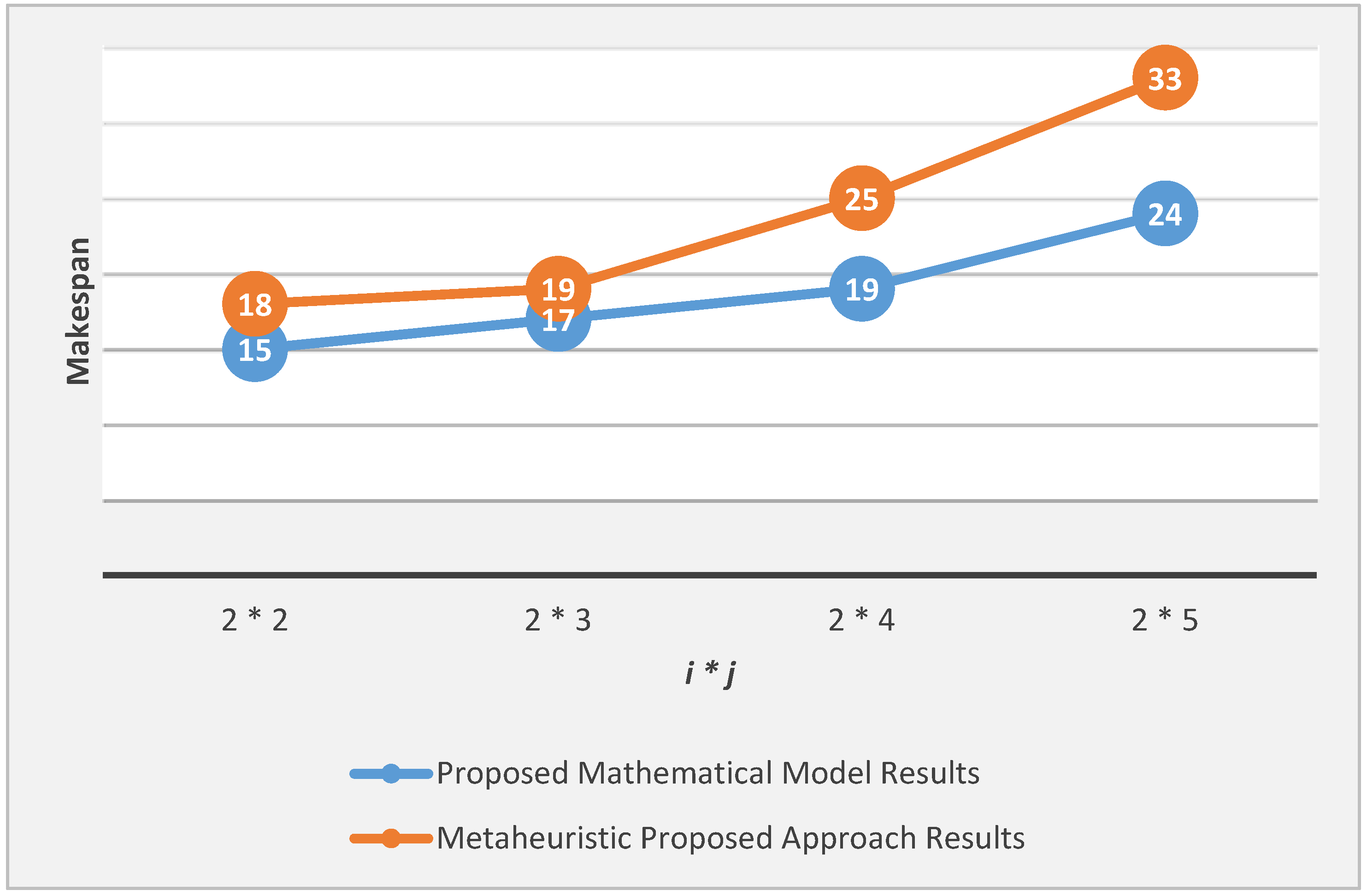
The effectiveness of the genetic algorithm is tested by evaluating the makespan computed with that determined by the mathematical model (through the Xpress optimizer). In order to make the comparison, we have computed the makespan for two machines as a function of the job number (Figure 13).

On the basis of the results shown in Table 7 and Figure 13, the GA yields a good average makespan compared to the optimal solutions given by the mathematic model. The actual computing time for each problem was nearly the same for the two resolutions of the frameworks.

8.3. Comparative Study

In this section, a comparison between the above approaches’ results and those given by the works of [21] is established. We have chosen this study to compare, since the authors deal with the same problem, which is the FMS scheduling problems, where the production process could be modeled by Petri net properties, but in different resolution framework conditions. In order to compare various parameter specifications under the same computational load, model performances are determined through the makespan value.

Li et al. [21] did not consider the availability constraint in their proposal. Results shown in

Table 8. Comparison of the two models applied with the availability constraints.

Case	Size $\mathit{i}\times \mathit{j}$	Lot Size	$\mathit{M}\mathit{s}$ [21]	$\mathit{M}\mathit{s}$
1	$3\times 3$	$1$	$43$	$36$
2	$5\times 6$	$1$	$64$	$57$
Processing time for Case 1		$5,3,3;5,4,5;4,1,3$
Processing time for Case 2		$1,2,4,5,1,5;5,2,2,3,4,1;5,4,5,2,4,2;2,3,5,3,1,3;3,3,4,3,3,2$
Maintenance periods for Case 1		$\left[2,7\right];\left[0,6\right];\left[10,13\right]$
Maintenance periods for Case 2		$\left[2,7\right];\left[0,6\right];\left[10,13\right];\left[20,23\right];\left[30,35\right];\left[41,43\right]$

illustrate the comparison of their model adding the constraints of availability and our mathematical model. On the basis of makespan ($Ms$) values, it can be concluded that the results given by our approach are in good agreement with those given by Li et al.’s [21] approach. In addition, the efficiency of our approach could also be highlighted by the fact that [21] assume that the order of jobs could differ in machines (more relaxed).

9. Conclusions

Reachability marking numbers increase exponentially, which leads to FMS state saturation. Consequently, previously-proposed models in the literature perform poorly. Therefore, in this study, we proposed a mathematical model, based on the decomposed $\mathrm{TPN}$ property, to solve the scheduling problem and minimize the processing time. In addition, a genetic algorithm is introduced, to provide efficiency solutions in the case of large-scale scheduling problems. Promising results indicate that the new model is efficient compared with similar models.

As perspectives, further studies should be considered to extend the proposed approaches for a parallel machine purpose with several practical constraints, such as limited buffer capacity.