Article

Resilient Modulus Characterization of Compacted Cohesive Subgrade Soil

1
Water Centre-Laboratory, Faculty of Civil and Environmental Engineering, Warsaw University of Life Sciences-SGGW, Warsaw 02-787, Poland
2
Department of Geotechnical Engineering, Faculty of Civil and Environmental Engineering, Warsaw University of Life Sciences-SGGW, Warsaw 02-787, Poland
*
Author to whom correspondence should be addressed.
Appl. Sci. 2017, 7(4), 370; https://doi.org/10.3390/app7040370
Submission received: 27 January 2017 / Revised: 14 March 2017 / Accepted: 27 March 2017 / Published: 7 April 2017

Abstract

:
Soil investigations concerning cyclic loading focus on the evaluation, in particular, of design parameters, such as elastic modulus, Poisson’s ratio, or resilient modulus. Structures subjected to repeated loading are vulnerable to high deformations, especially when subgrade soils are composed of cohesive, fully-saturated soils. Such subgrade soils in the eastern part of Europe have a glacial genesis and are a mix of sand, silt, and clay fractions. The characteristic of, e.g., Young modulus variation and resilient modulus from repeated loading tests, is presented. Based on performed resonant column and cyclic triaxial tests, an analytical model is proposed. The model takes into consideration actual values of effective stress p′, as well as loading characteristics and the position of the effective stress path. This approach results in better characterization of pavement or industrial foundation systems based on the subgrade soil in undrained conditions. The recoverable strains characterized by the resilient modulus Mr value in the first cycle of loading was between 44 MPa and 59 MPa for confining pressure σ’3 equal to 45 kPa, and between 48 MPa and 78 MPa for σ’3 equal to 90 kPa. During cyclic loading, cohesive soil, at first, degrades. When pore pressure reaches equilibrium, the resilient modulus value starts to increase. The above-described phenomena indicate that, after the plastic deformation caused by excessive load and excess pore water pressure dissipation, the soil becomes resilient.

1. Introduction

The structures which are subjected to dynamic and repeated loads are mostly industrial foundations, railroads, and pavement. Such structures are based on occasionally highly plastic soils, where their origin is connected with a glacier. Such cohesive soils can be found in central and northeastern parts of Europe.
Bituminous pavements are based on rigid and granular layers, to provide the optimal distribution of traffic loads [1]. Nevertheless, soft cohesive subgrade soils, even under low loading conditions and after improvement, still develop some deformations [2].
The uneven settlement or rutting which can be observed as a premature exceeding of the serviceability limit state is caused by such deformation in the subgrade and, therefore, in the sub-base layer. The deformation of soils under dynamic and cyclic loading conditions is important to study [2,3,4,5].
In the case of a pavement construction on an embankment based on soft soil, the permanent deformation characteristics caused by traffic become an important factor, which impacts the design life and maintenance of pavement [6,7].
The long-term cyclic loading and short-term dynamic loading characterizes the traffic excitations. The typical strains in the base and sub-base vary from 0.01% to 1%. The strain change range in subgrade soil layers vary from 0.003% to 0.6% [8,9].
The long-term loadings, defined as a “quasi-static loading”, cause long-term settlements and creep processes to occur due to the dissipation of loading energy as a plastic strain. The dynamic loadings caused by traffic may occur in the form of short-term deformation of layers, characterized by the small permanent strain and the behavior of layer, which may be seen as reversible [1,10,11,12]. The evolution of modulus value during cyclic lading shows different characteristics under certain strain range. Therefore, the popper adjustment of the moduli value is important.
The design method of pavement layer thickness is based on the mechanistic pavement analysis, which uses the multilayer linear elastic model and a cyclic triaxial test. The laboratory tests conducted on the pavement layer material leads to the definition of the actual soil mechanical behavior under cyclic loading by simulating the in situ conditions [13,14,15,16,17].
The calculations of characteristic values for the pavement design purposes, in the mechanistic method, concerns the estimation of the Young’s modulus E and Poisson ratio υ. The resilient modulus Mr, defined as the unloading modulus of the hysteresis loop after many cycles of repeating loads, is a stiffness measurement of pavement layers. The Mr value is connected with the non-linear elasticity model [18,19,20,21]. The plastic displacement which is another important part of pavement design and is calculated mostly on the basis of empirical models, based on the results of cyclic triaxial tests, which present the plastic strain function of a number of cycles [22].
The response of soil to repeated loading is stress dependent, therefore, the resilient modulus value is also stress-dependent. The low pressure conditions during dynamic tests results in small strain and elastic response of the soil, provided that the strain amplitude does not exceed 10−4%. One of the best methods of obtaining this kind of loading and separating the stress-strain elastic relation is propagating in the soil small amplitude stress waves [23,24]. The linear stress-strain behavior below the strain level being equal to 0.001% was observed for uncemented granular soils [25,26].
The small-strain characteristic modulus is called the “maximum Young’s modulus” Emax or the “maximum shear modulus” Gmax. The Gmax value corresponds to the linear elastic region of strain, where no plastic strains occur. If the shear force is high enough, the G value starts to deviate from Gmax [27].
In the small-strain, elastic zone the shear modulus is calculated using Equation (1):
G = ρ V S 2 ,
in which ρ stands for soil density and Vs stands for the shear wave speed.
The shear wave speed is estimated using, e.g., the bender element test (BE). The bender elements are piezoelectric cantilever strips, which are placed on top of the soil specimen’s bottom side. The electric signal produces compressional (P) and shear (S) waves. The wave produced by the bender element propagates through the soil sample and induces a voltage in the second bender element. The wave propagation data recorded by the emitter and receiver of the bender element as a function of time leads to estimating the shear and compression wave velocities [28].
The repeated loading conditions in which the plastic strain occurs takes place in intermediate and large strain zones. The resilient modulus Mr is based on elastic theory, although subgrade materials, themselves, are not elastic. If the load is small enough, after a large number of repetitions, the soil can behave in an elastic manner; however, the deformation is nearly fully, but not fully, recoverable [29,30,31,32]. The phenomenon of plastic deformation decreases during cyclic loading and is connected with the shakedown concept, while the state after numerous cycles, in which no permanent deformation occurs, is called the “resilient state”. This specific elastic state is characterized by resilient modulus Mr.
The influence of such factors as confining pressure, deviator stress, moisture, saturation degree on resilient modulus value was reported by many studies [33,34,35,36,37,38]. The conditions under which the soil subgrade works are characterized by long-term repeating loads.
The Mr value is calculated using Equation (2):
M r = σ m a x Δ ε r ,
in which Δσ stands for the deviator stress and Δεr stands for the recoverable strain. The resilient modulus value can be obtained by repeat loading triaxial tests of the tested soil. Numerous methods and numerical models have been proposed in order to obtain the Mr value [39,40]. One of them is the k-θ model, called the “Uzan-Witczak model”, which describes the resilient modulus, characteristic for varying confining pressure [41].
This model is applicable for various types of soil. Its coefficients (k1, k2, and k3) for a certain type of soil remain the same, in regard to the stress state. The Uzan-Witczak model equation is presented in the Equation (3):
M r = k 1 p a ( θ p a ) k 2 ( q m a x p a ) k 3 ,
in which θ stands for the bulk stress θ = σ x + σ y + σ z = 3 σ c + Δ q , where σc is confining pressure, Δq is stress magnitude, pa stands for the atmospheric pressure (normalizing factor), qmax is the stress deviator equal to q m a x = σ 1 σ 3 ; k1, k2, and k3 are regression constants that are a function of the soil properties [42].
The resilient modulus value of granular materials is dependent from several parameters, among which the most important are the stress level, confining pressure and moisture content, the Mr value decreases along with the increase in water content [43].
The Mr value in certain, constant physical soil conditions, changes with strain level. A method for describing this phenomena is degradation curve which presents a change of the modulus at a given strain level to the maximal material modulus [44].
The difference between the elastic moduli in small-strain and plastic zones is presented in Figure 1.
In this article, the resilient modulus Mr characteristic for cohesive soils was presented and a new analytical model for resilient modulus calculation is proposed. The analytical model takes into account actual values of effective stress p′, excess pore water pressure, the loading characteristic (for example, qmax) and the position of the effective stress path. The proposed model describes more exact the phenomena of modulus development during cyclic undrained conditions. The cohesive soil deformation characteristics, which are common to glacial till in Northern and Eastern Europe, is presented. Tests performed on this type of soil are rather rare.
Tests which characterize the stiffness change from small to large strains consist of resonant column (RC) and torsional shear (TS) tests in a small strain range were performed with the purpose of estimating the Young modulus E degradation curve. The intermediate and large strain zones were specified by conducted cyclic triaxial tests (CTRX. Such tests are one of the pioneering methods for this type of soil.
The impact of cyclic loading in the plastic zone was investigated and an occurrence of the quasi-elastic response after numerous repetitions was studied. During the unloading stage, the hysteresis curve can be specified by different tangent resilient modulus values in this study, called Mr max. The Mr max characterizes the elastic response during the first phase of unloading, in which the modulus value is the greatest.

2. Materials and Methods

For the tested material, cohesive soil, standard laboratory tests were conducted to classify the soil and determine its physical properties. The tests consisted of particle size analysis, consistency limits, and the Proctor compaction test was conducted.
The particle size analysis led to recognising the cohesive soil as a sandy clay (saCl), by performing tests based on sieve and aerometric analysis (the Bouyoucos method using a modification made by Casagrande), in accordance with the EUROCODE 7 [45] standard. Test results are shown in Figure 2.
In terms of World Reference Base for Soil Resources—WRB—the tested soil can be recognised as albeluvisoil (AB). The soil was deposited by glacial processes. The sandy clay in natural conditions is unconsolidated glacial till. This type of soil shows no stratification.
The liquid limit and plasticity limit test were conducted in accordance to [46]. On the basis of six sets of tests using the Casagrande apparatus with varying moisture content the liquid limit LL was established as being equal to 18.9%, classifying this soil as a clay with low plasticity. The plasticity limit PL was equal to 10.3%.
The optimum moisture content was conducted using the AASHTO T99 [47] procedure. It was achieved by a compaction in the Proctor mold whose volume is equal to 2.2 dm3. Standard energy of compaction, equal to 0.59 J/cm2, was used. Optimum moisture content for sandy clay was equal to 10.2% and the maximum dry density at optimum moisture content reached a value of 2.09 g/cm3. Table 1 presents the results of physical and mechanical tests conducted on sandy clay.
Bender element (BE) and torsional shear (TS) tests in a resonant column apparatus led to the estimation of the shear modulus, Young modulus and, finally, the Poisson ratio.
After determining the properties of the soil, several series of triaxial tests under cyclic loading conditions were conducted. The tests were performed on compacted sandy clay, with optimal moisture conditions, in accordance with the Proctor method. The maximum dry density of soil samples was equal to 2.09 g/cm3.
In this paper two kinds of tests, one using the RC device and second using the CTRX were ran. However, the tests were conducted with an attempt to maintain similar testing conditions during both measurements. Initial effective confining pressure σ’3, was set to be 45 kPa, 90 kPa, and 135 kPa during all of the conducted tests. The examined soils were initially saturated, and the B values measured in the triaxial specimens exceeded 0.95, which means full saturation of sandy clay specimens. Subsequently, the tested specimens were consolidated to the set state of stress σ’3.
Repeated loading triaxial (CTRX) tests were carried out with a triaxial apparatus from GDS instruments (GDS, Hampshire, UK). The device is suitable for cylindrical soil specimens of 7 cm in diameter and 14 cm in height. Samples were fully saturated, and a B-value equal to, or greater than, 0.95 was assured at each measurement.
Specimens were then subjected to isotropic effective confining pressures of 45 kPa, 90 kPa, and 135 kPa and consolidated. The cyclic-test procedure consisted of applying an average deviator stress value qm superimposed to a forward-moving pulsating sine wave with constant stress amplitude qa. Details of the experimental design are shown in Table 2. Repeated loading triaxial tests were conducted under the consolidated-undrained (CU) conditions. The frequency used during the tests was equal to 1.0 Hz.
The tests were performed in a multistage manner. After the first series of tests (105 cycles), further stages were conducted. Each stage was characterized by characteristic deviator stress q values.
The cyclic stresses and initial confining pressure levels were used to define the effects of cyclic loading on soil behavior.
The resonant column has a fixed-free configuration. The specimen is fixed to the pedestal at the bottom end, and the other end is connected to the drive plate, while the top cap remains free. This system is provided with a testing unit (testing chamber), control computer, back pressure system, cell pressure controller, resonant column controller, and a data acquisition box [48,49,50].
Immediately after the first mode is found, the measurements of the resonant frequency (Fr) of the vibration amplitude are made. The sinusoidal torsional vibration at variable frequency is applied in a rotary manner by a device which causes such excitations. Subsequently, these measurements are combined with the specimen size and equipment characteristics in order to determine the shear wave velocity (VS), shear modulus (G), and shearing strain amplitude (γ). Based on the elastic wave propagation, the fundamental data-reduction equation, Equation (4), can be established:
I I 0 = ( ω r L V S ) tan ( ω r L V S ) ,
in which I and I0 stand for the moments of specimen inertia and the driving system, respectively; ωr, the natural frequency, stands for the system, and L stands for the length of the sample. In this study, the specimens of a typical size were used, i.e., representing 70 mm in diameter and 140 mm in height. Upon calculating the shear wave velocity, the shear modulus could be computed from Equation (1). The RC apparatus can perform at the resonant frequency, TS, and BE tests on the same specimen, without change of device settings.
During TS tests, the sample was subjected to small cyclical torsional motion due to a coil-magnet system at the RC. The shear stress was calculated by the torque generated this way. The shear strain levels were determined from the twist angle of the soil sample, as measured by a proximitor. The shear strain was controlled by applying a voltage between 0.004 V and 1 V to the coils, which generated a shear strains between 0.0001% and 0.003%.
The TS tests were conducted with the application of a sinusoidal load wave with frequencies of 0.1, 1 and 10 Hz. The shear modulus G and damping ratio D were estimated for all three frequencies. For measurements at 0.1 Hz and 1 Hz, ten cycles were taken into account for G and D calculations. For the 10-Hz frequency, 100 cycles were used. The range of the tested amplitudes varied between 0.005 V and 0.6 V.
The properties of sandy clay samples are summed up in Table 3. The descriptive statistics covers mass, dimensions, and basic physical parameters. The results of standard deviation calculations show a high repetition of dry density and moisture content. The differences in sample dimensions are caused by the compaction technique in the Proctors mold designed for samples used for triaxial tests.

3. Results and Discussion

The triaxial tests were performed in order to, above all, designate the resilient modulus Mr of sandy clay under the changing test conditions. The second objective of the test was to estimate the maximal value of resilient modulus Mr max during the first stage of unloading. The permanent strain accumulation was also analyzed. The axial strain ε1 development during the tests conducted in the triaxial apparatus are presented in Figure 3a–c.
The strain observed during this tests indicate three possible ways of soil responding to such loads. The deformation characteristic with the number of cycles N is distinguished between a stepwise failure, shakedown, and abation [51]. The concept of deformation which occurs during cyclic loading was later developed to refer to shakedown theory. The three possible categories of material response are:
-
Plastic shakedown, characterized by a rapid decrease of the plastic strain rate, this phenomena is followed by an equilibrium state and fully resilient strains are observed.
-
Plastic creep is observed when plastic deformation are observed in each cycle or in a cumulative plot of plastic deformation against the number of cycles the increase of deformations are observed.
-
Incremental collapse, when plastic deformations are great and failure is achieved in a low number of cycles.
The tests performed under constant radial stress equal to σ’3 45 kPa, in which deviator stress amplitude qa was equal 5.30 kPa and maximal deviator stress qmax was equal 31.90 kPa, resulted in low strain accumulation and shakedown response. The same permanent deformation characteristic was observed in case of tests 1.2, 1.3, 2.1 to 2.4 and 3.1 to 3.5. The second kind of soil response to cyclic loading, which is plastic creep, was recognized in test numbers 1.4 to 1.6, 2.5 to 2.6, and 3.6 to 3.9. The strain accumulation was higher and a growing tendency of strain accumulation was observed. The incremental collapse phenomena was preceded by the occurrence of shakedown. In other words, plastic creep was not observed in Stage 1.7 and 2.7. The last phenomenon, incremental collapse, occurred in Stages 1.8 and 2.8, but not in the case of tests in σ’3 equals to 135 kPa. The strain accumulation displays characteristic growth, which led to failure.
All three phenomena were present in the performed tests. The characteristic method of deformation development leads to various resilient modulus values and the resilient response, which can be compared to the elastic phase in the small strain zone.
Figure 4a–c show the effective p′ stress paths obtained during tests in the radial stress equal to σ’3 45 kPa, 90 kPa, and 135 kPa, respectively.
The stress path plots show distinctly different mean effective stress paths during cycling and provides a tool to analyze the stress-path evolution. Such evolution happens as a result of pore pressure generation, which increases after numerous cycles, which cause the movement of the stress path toward the critical state line. When the critical state is reached, the stress path moves opposite to the deviator stress axis.
During cyclic loading (σ’3 = 45 kPa), the stress path moves toward the deviator stress axis in the first three stages. After the third stage of loading, the stress path starts to move in the opposite direction. The pore water pressure decreases, which was the result of the increase in porosity value. The incremental collapse was observed. This process lasts during tests 1.4 to 1.6. Test 1.7 was characterized by a smaller maximal deviator qmax increase. During this test the plastic strain rate was lower (see Figure 3a), as was the stress path rate. This phenomenon was caused by lower maximal deviator stress than the critical state deviatoric stress in this condition. The same observation can be made when the 2.7 test is analyzed. Conditions under σ’3 equal to 135 kPa shows that the critical state is reached by the soil sample in Stage 3.9 (see Figure 4c).
The loading conditions of conducted cyclic triaxial tests which are called constant stress conditions, lead to a critical state but this state did not last during the time of the test, which can be observed as strain development during cycling. The strain rate decreases and after around 103 repetitions the purely resilient statistic can be observed.

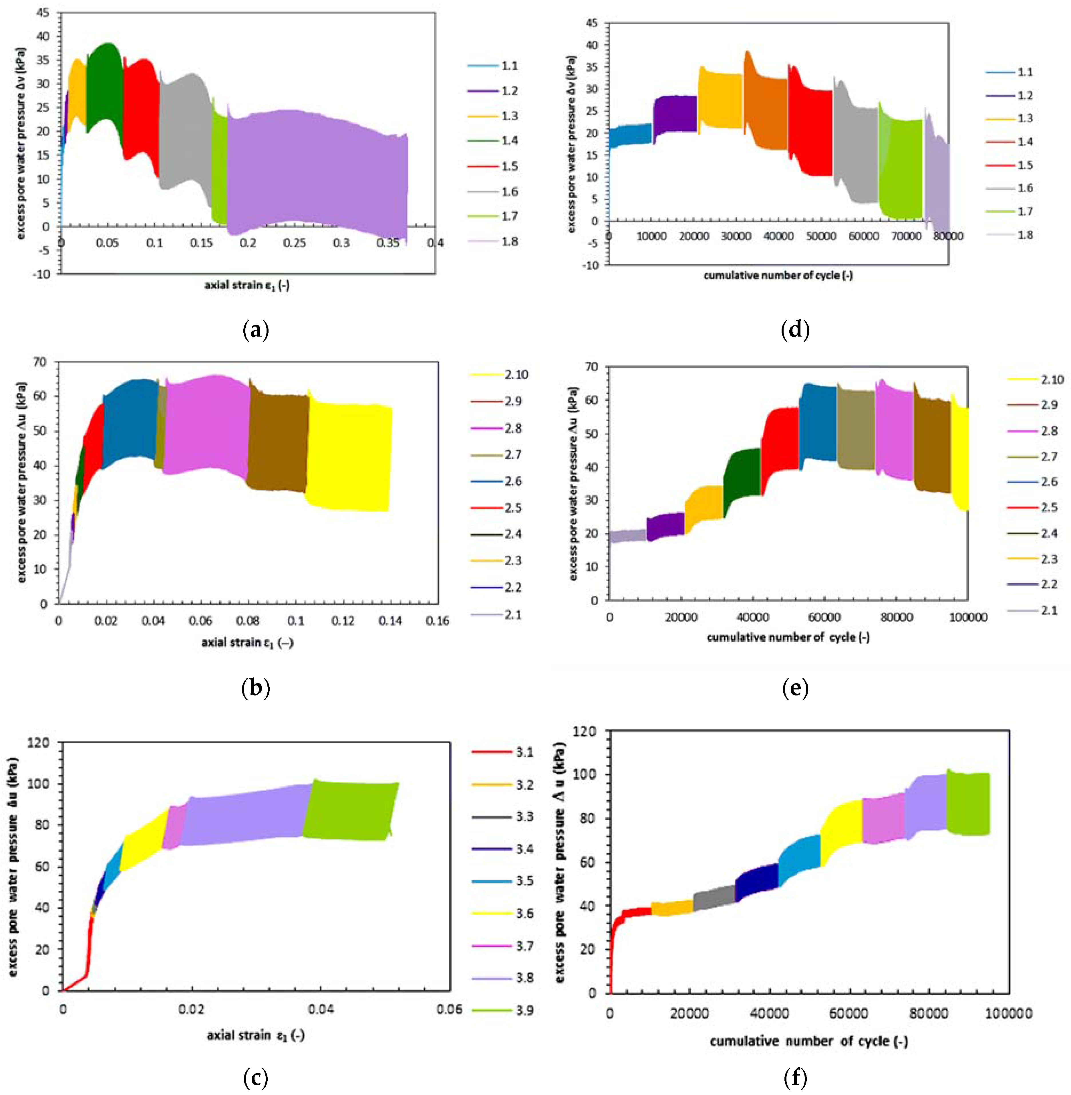
3.1. Pore Pressure Analysis

During undrained tests, the pore pressure was not expected to dissipate due to leakage. This happened because drainage was kept steady by pressure and volume controllers. However, experiments have shown otherwise (see Figure 5a,b).
The pore water pressure develops in a similar scenario for the three radial stress test conditions. At tests 1.1, 2.1, and 3.1 the pore water pressure rises due to the first load cycle, which causes the greatest pore pressure build up. After this event, the pore water pressure rises during cyclic loading until the critical state is achieved. During tests 1.1 to 1.3, tests 2.1 to 2.5, and tests 3.1 to 3.8, the change of the deviator stress value caused the response of the pore water pressure, raising the pressure. After the abovementioned tests, the increase of qmax led to another behavior. In the first cycles the pore water pressure increases, which causes the development of plastic strain. This phenomenon is observed as a pore water pressure decrease due to changes in porosity.
When pore water pressure reaches the lowest value in this phase, a hardening process begins to occur. This phenomena can be recognized as the pore water pressure builds up.
Nevertheless, indirect conclusions can be drawn from the analysis of the accumulation of plastic strains, which are presented in Figure 3a–c.

3.2. Resonant Column Test Results

The maximal Young modulus value was obtained by performing the torsional shear (TS) test and resonant column test (RCA). The frequency in TS tests was equal to 1 Hz. The plot of the Young’s modulus at different radial stresses is shown as a function of γ in Figure 6. The results show the low dependence of Emax on the radial stress value.
The maximum value of Young modulus from RCA and TS tests for radial stress σ’3 equal to 45 kPa was 135.5 MPa, for σ’3 equal to 90 kPa, Emax was 218.2 MPa.

3.3. Analysis of Resilient Modulus Value

The hysteresis loops were analyzed and the value of Mr was established for nineteen tests. The additional values of Mr max, which characterizes the modulus with maximal slop on the stress-strain plot, were also calculated (see Figure 7). The purpose of these calculations was to evaluate the correlation between maximal resilient modulus and Emax. The resilient modulus had different values for each of the applied deviator stress levels, and the Mr max values were also different for each test.
The recoverable strains characterized by the resilient modulus Mr are presented in Figure 8a–c for tests in σ’3 equal to 45 kPa, 90 kPa, and 135 kPa, respectively. The Mr value in the first cycle was between 44 and 59 MPa for confining pressure σ3 equal to 45 kPa and between 48 and 78 MPa for σ’3 equal to 90 kPa. For σ’3 equal to 135 kPa the Mr value was between 45.0 to 81.1 MPa. During cyclic loading, the resilient modulus value decreases to around 103 cycles. Then, in the case of plastic creep strain response, the Mr value increases in the rest of the tests.
The resilient modulus Mr decrease was caused by strain development between 102 and 103 cycles. This can be observed as the Mr value decreases on plots 8a–c and indirectly on plot 3a–c. After this stage, the Mr value increases. The reason for that is the increase of stiffness which can be observed as smaller resilient strains in one cycle. During this phase, the stress path has not changed its value (see Figure 5c,d), the equilibrium state is achieved, and no further changes of the resilient modulus value occurs.
The differences in the Mr value are clearly dependent from the deviator stress levels, which causes decreased soil strength in further steps during this test. The deviator stress also causes different responses of the soil. In the case of the tests conducted in radial stress σ’3 equal to 45 kPa, the Mr average values was between 41.8 to 70.5 MPa. Four stages of cyclic loading were characterized by lower values of Mr and were between 41.8 to 49.9 MPa. The Stages 1.5 to 1.8 showed another Mr value development. The resilient modulus rises from 47.6 MPa to 70.5 MPa. The Mr value for tests conducted at radial stress σ’3 equal to 90 kPa ranged between 43.0 and 65.3 MPa. The average value of resilient modulus in first stage of repeating loading varies form 44.7 MPa to 56.3 MPa. The test results for σ’3 equal to 90 kPa indicate that the Mr value decreases with rising deviator stress qmax, which is not so clear in the case of tests where σ’3 is equal to 45 kPa. After the specimen rises to a critical state, the Mr value rises from 43.0 to 55.8 MPa. The tests performed in σ’3 equal to 135 kPa show other characteristics. The average resilient modulus in the first stages is low and rises in Stages 3.2 and 3.3, where it reaches a maximum value. In Stages 3.4 to 3.9 decreases occur due to pore pressure. Detailed information about the resilient modulus values are presented in Figure 9a–c.

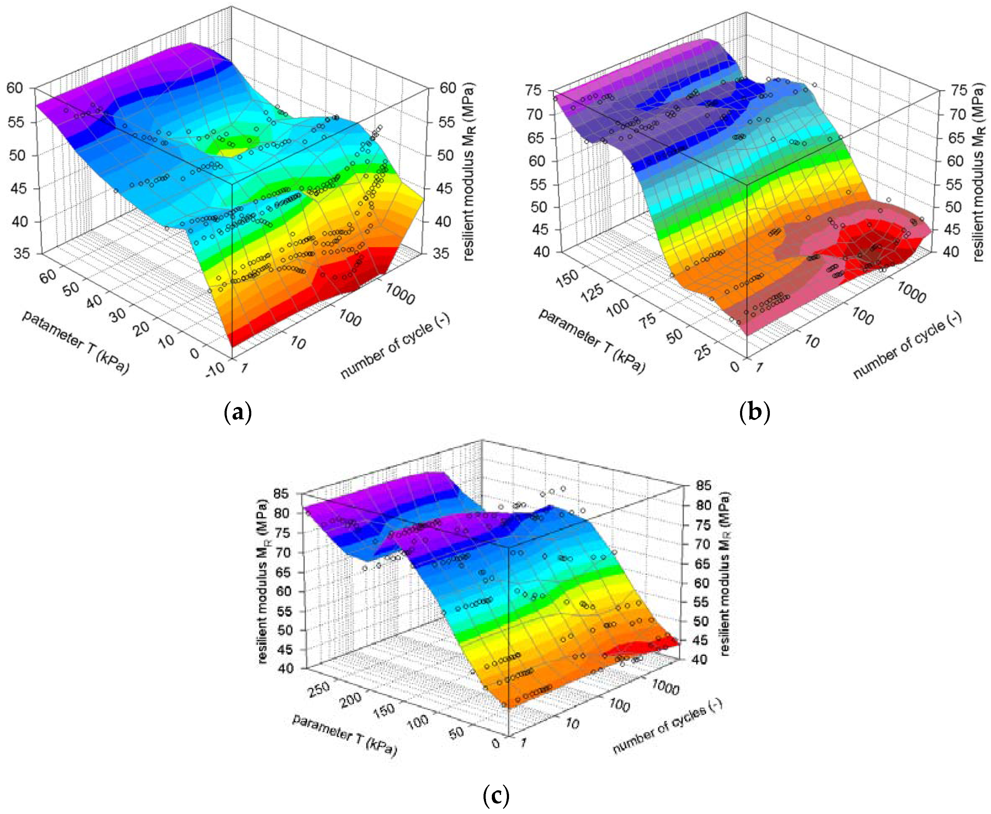
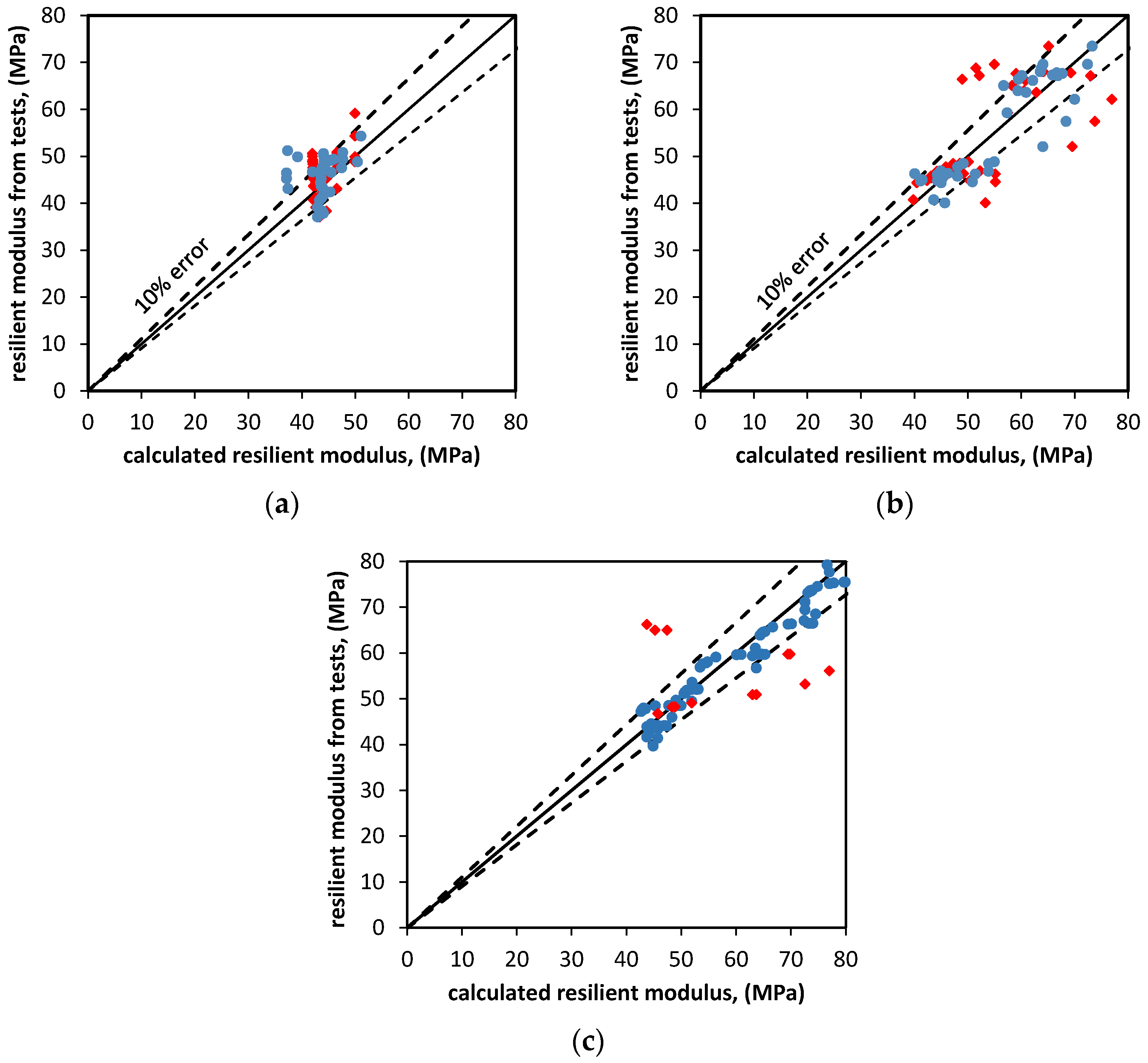
3.4. Analytical Model for Mr Calculation

Calculations on the average resilient modulus value (Mr avg) and analysis of effective stress paths (see Figure 4a–c) led to the estimation of the function describing the change of resilient response of tested soils as a function of the maximal deviator stress in the actual mean effective stress conditions.
The stress paths ‘critical state line for both tests in radial stress σ’3 conditions was employed for the model. The inclination M of the critical state line was calculated based on Equation (5):
M = q m a x p ,
in which qmax is stated as the maximal deviator stress in the actual mean effective stress conditions.
The M parameter is equal to 2.4. For characterization of how distant the actual maximal deviator stress is from the maximal deviator stress in the critical state, the T parameter is introduced. The maximal deviator stress qmax(p) is a value of deviator stress which must occur to reach the critical state. Equation (6) presents the abovementioned parameter:
q m a x ( p ) = M p ,
The T parameter, therefore, is simply the difference between qmax(p) and qmax from Equation (7):
T = q m a x ( p ) q m a x
The T parameter change is presented in Figure 10. The figure plots the value of the resilient modulus and T parameter in 3D space. Note that the resilient modulus is almost independent from the number of cycles. Additionally, the Mr value corresponds to the value of the T parameter. This phenomenon is very similar for tests in the effective confining pressure σ’3 equal to 45 kPa, 90 kPa, and 135 kPa. This fact strongly suggests that the change of Mr can be modeled in a reasonable manner through the use of an equation involving the T parameter and number of cycles N.
Based on the test results, the selection of parameters to formulate the resilient modulus equation should be conducted carefully. On one hand, the formula must have its limitations, and the results derived from their use must be carefully interpreted. On the other hand, the use of the resilient modulus formula which have parameters significantly different for each test condition results in different Mr values.
According to previously-presented test results, the level of resilient modulus in cohesive soil subjected to cyclic loading can be estimated through the combination of the number of repeated loading and T parameter.
The linear formula based on this two parameters and constants which characterize the cyclic loading conditions is presented in Equation (8):
M r = k 1 + ( 1 k 2 E m a x N ) + ( χ Δ u 1 ) k 3 T
The χ parameter is termed amplitude ratio (MPa) and can be calculated based on Equation (9):
χ = q m q a = 1 + R 1 R
The Δu1 is the excess pore water pressure in the first cycle in MPa. The k1, k2, and k3 indicators are material constants. Figure 11 summarizes the target resilient modulus obtained during the tests and calculated Mr value based on Equation (8).
The resilient modulus was calculated from Equation (8). This is confronted by the Uzan-Witczak model. The results of the Uzan-Witczak resilient modulus Mr was calculated based on Equation (2). The result show that the resilient modulus calculated based on Equation (8) (constants k1 = 43, k2 = 10, k3 = 0.2) better fits the obtained data. The Uzan-Witczak model parameters were fitted for this study in each test. The k1, k2, and k3 parameters were equal to 0.19, 0.91, and −0.45, respectively, for σ’3 equal to 45 kPa, 0.15, 0.91, and −0.45 for σ’3 equal to 90 kPa, 0.4, 0.1 and −0.31 for σ’3 equal to 135 kPa. The results of resilient modulus calculation also shows that if we consider a 10% error level for Mr estimation, in almost all cases the resilient modulus is in this range.
The proposed resilient modulus model as well as the Uzan-Witczak, can be exploited in the analysis and design of pavement systems. This analytical models is motivated by the observation of the cohesive soil response to cyclic loading. It is obvious that the Uzan-Witczak model was created for unbound granular materials and, therefore, the resilient modulus calculation results must not be the same as the test results.
The analytical model presented above takes into consideration the actual values of effective stress p′ (parameter T), actual excess pore water pressure in reference to initial conditions before cyclic loading Δu1, the loading characteristics (qmax and χ), and the position of the effective stress path (the T parameter). This approach results in better characterization of pavement or industrial foundation systems where undrained conditions in the subgrade soil may occur.

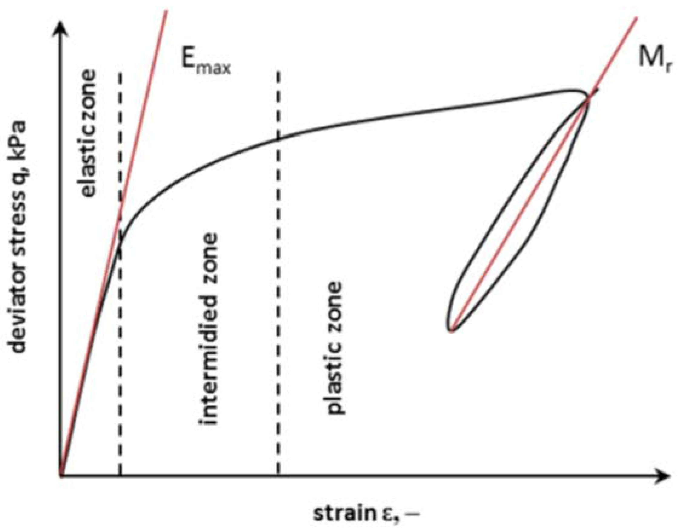
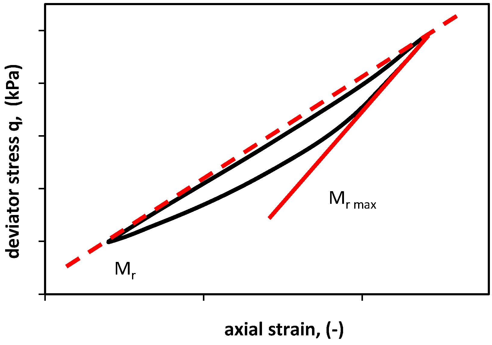
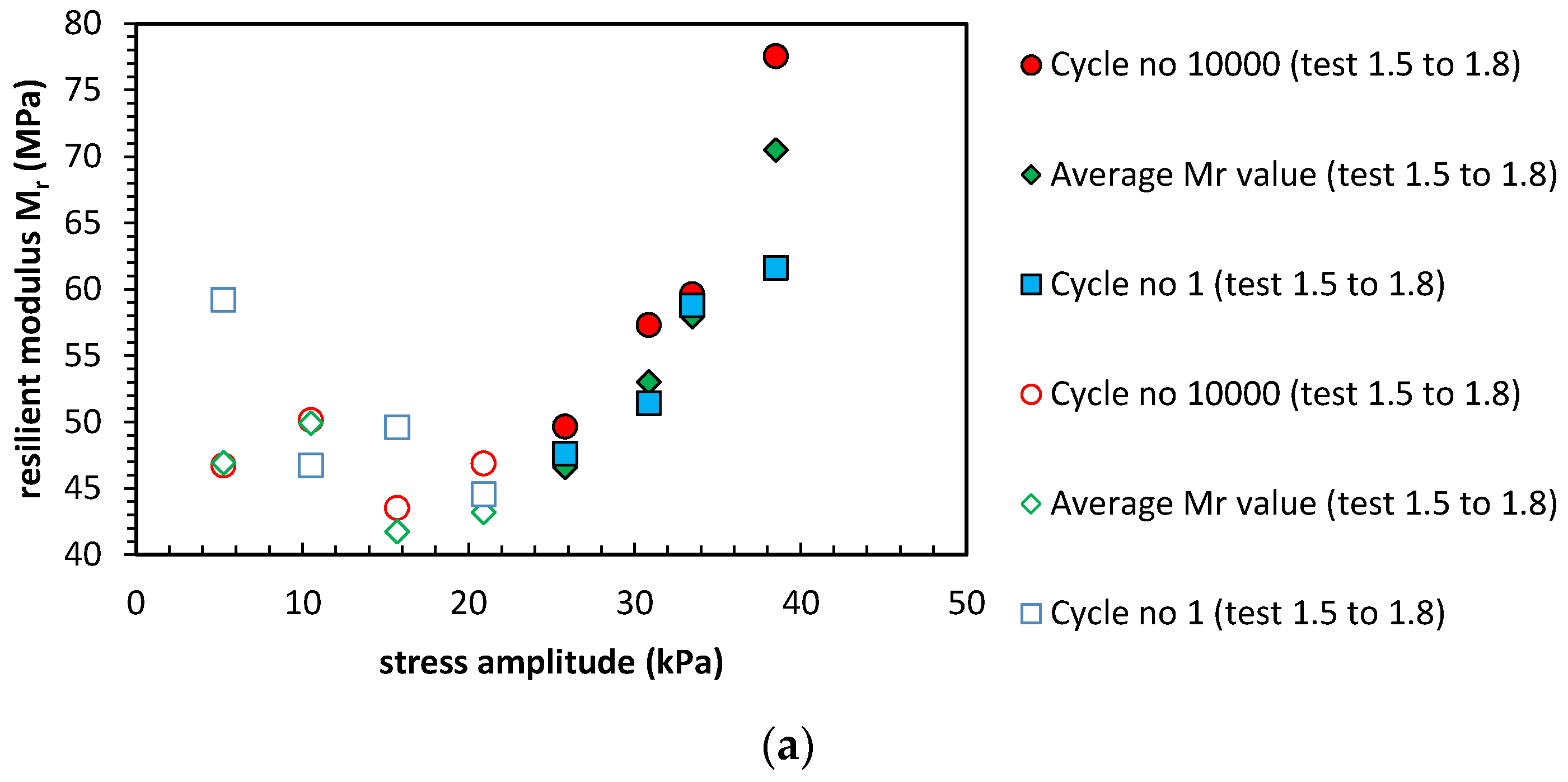
3.5. Maximum Resilient Modulus Value Analysis

The maximum resilient modulus Mr max change for σ’3 = 45 kPa and σ’3 = 90 kPa versus axial strain Figure 12a,b. Maximum resilient modulus Mr max during the test follows the same pattern for σ’3 equal to 45 kPa and 90 kPa. In the first cycles of tests 1.1 and 2.1, the Mr max degraded to a constant value after around 20–30 cycles. This occurrence is caused by excess pore pressure generation. When pore pressure reaches a constant value, the Mr max stabilizes and remains constant until the end of the test. The interval between the maximal and minimal Mr max values is the highest in the case of tests in the small strain zone. When the stress path moves towards the critical state path, the response of the soil changes.
The soil material in the critical state, at first, degrades. After this stage, when excess pore water pressure caused by a new amount of loading is dissipating, the maximum resilient modulus Mr max remains almost constant by around 1 × 10³ to 2 × 10³ cycles. When pore pressure reaches equilibrium, the maximal resilient modulus value starts to increase. Indirect conclusions can be drown from Figure 5a–d. The above-described phenomenon indicates that after the plastic deformation occurrence caused by excessive load and excess pore water pressure dissipation, soil becomes resilient and the maximal resilient modulus Mr max starts to increase.
The maximal resilient modulus value at third stage characterizes the high interval. This occurrence is caused by the small strain in this area in which measurements are difficult to maintain by the triaxial cell.
Nevertheless, Figure 12a,b show a comparison of the resonant column test results and cyclic triaxial test results. The degradation curve, which shows how the Young’s modulus E degrades during shearing test, fits for with maximum resilient modulus during the second stage of the above-described phenomena.
Degradation of the soil’s Young’s modulus value is caused by greater stress or strain amplitude. In cyclic triaxial tests, for maximum resilient modulus, the strain amplitude is greatest during the first stage of the test where the pore pressure rises and plastic strains occur. Therefore, the proper characteristic of the soil’s Young’s modulus degradation, in the case of the performed cyclic triaxial tests, is evident only for the first stage of tests where no critical state occurs, or for the second stage of tests where the critical state was noted.

4. Conclusions

The geotechnical design of pavement constructions need to also take into account the deformation properties of soils. The fundamental geotechnical concepts, like the strain level or deviator stress quantity, should be taken into consideration. The results presented in this paper illustrate the cohesive soil resilient modulus Mr and maximum resilient modulus Mr max. The test results lead to the following conclusions:
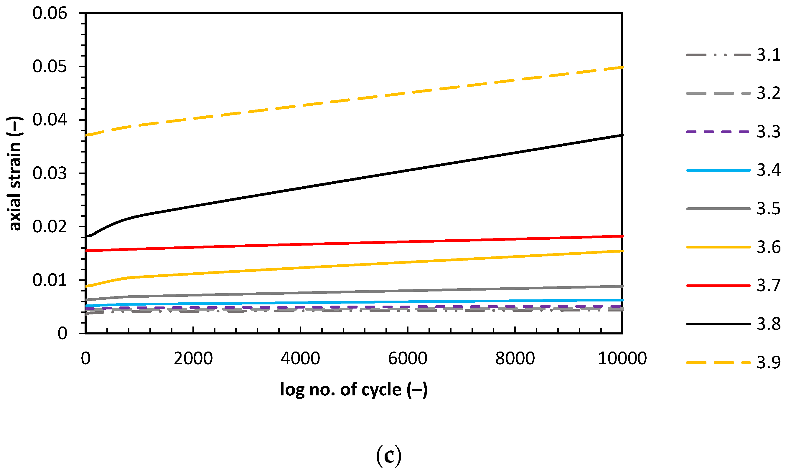
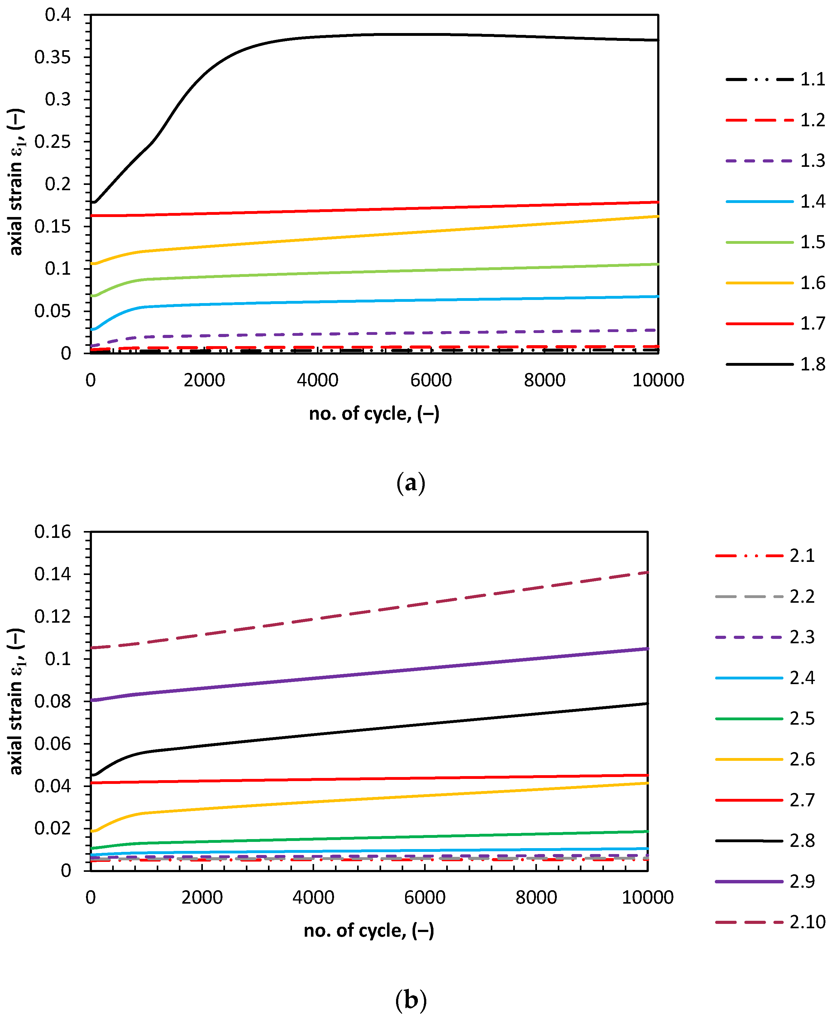
  • The strain observed during this test indicates three possible ways of soil the respond to cyclic loading. Under the low deviator stress amplitude, low strain accumulation is observed. In intermediate deviator stress amplitude levels, the strain accumulation was higher, the growth of strain accumulation can be observed. The plastic strain accumulation presents a characteristic growth tendency, which is caused by pore pressure development.
  • During the cyclic triaxial tests the stress path moves towards the deviator stress axis in the first few stages. When critical state of soil is achieved, the stress path starts to move in the opposite direction. The critical state did not last during the entire time of the test, which can be observed as plastic strain development during cycling. The strain rate decreases and, after numerous cycles, the purely resilient state can be observed.
  • The pore water pressure develops in a similar scenario for three radial stress test conditions. At the first stages of the tests the pore water pressure rises due to the first load cycles, which cause the greatest pore pressure build up. Later, the pore water pressure develops through further stages of cyclic loading until the critical state is achieved. When pore water pressure reaches the equilibrium state, a hardening process begins.
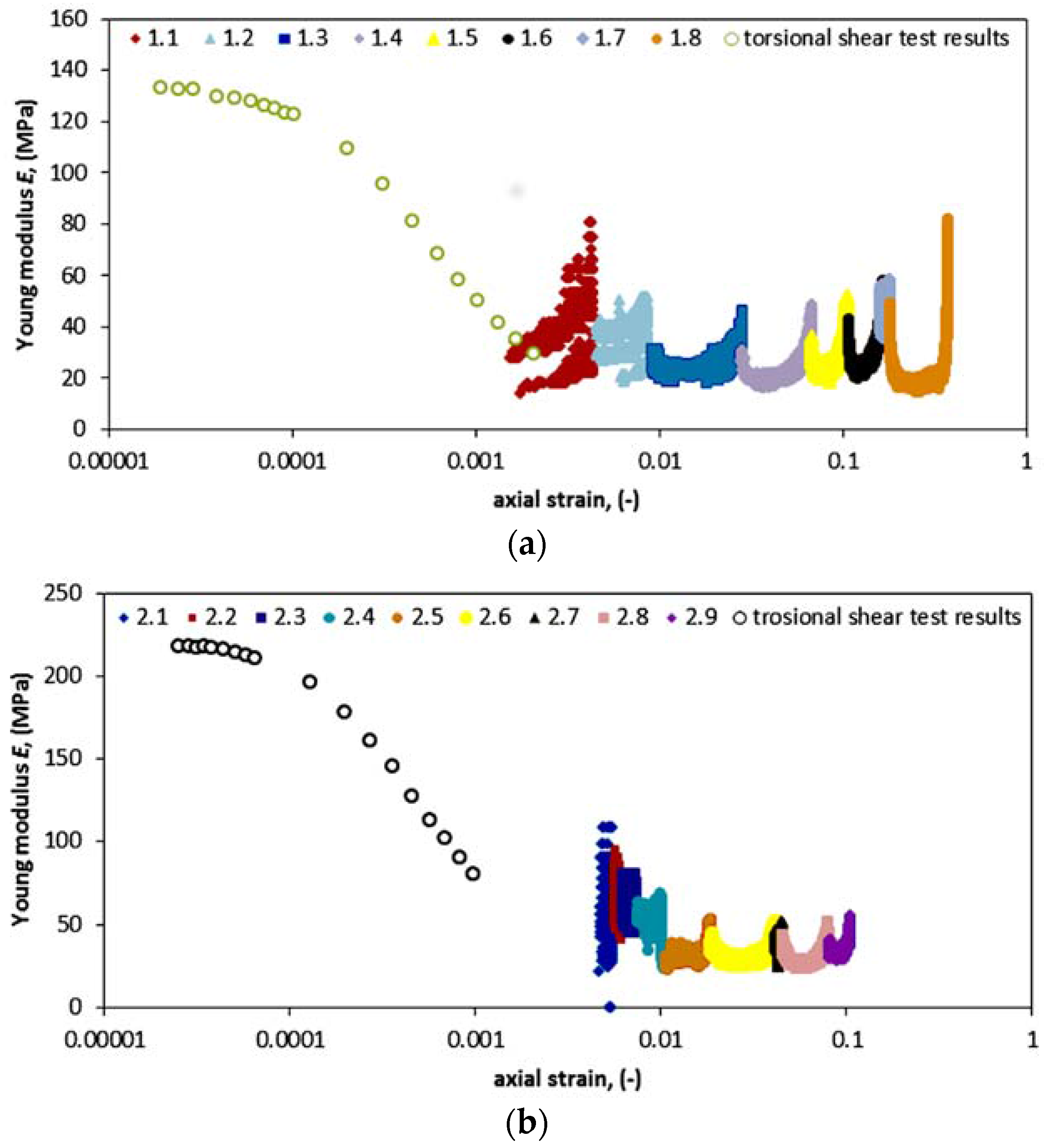
  • The maximum value of the Young’s modulus from RCA and TS tests for radial stress σ’3 equal to 45 kPa was 135.5 MPa, and for σ’3 equal to 90 kPa, Emax was 218.2 MPa.
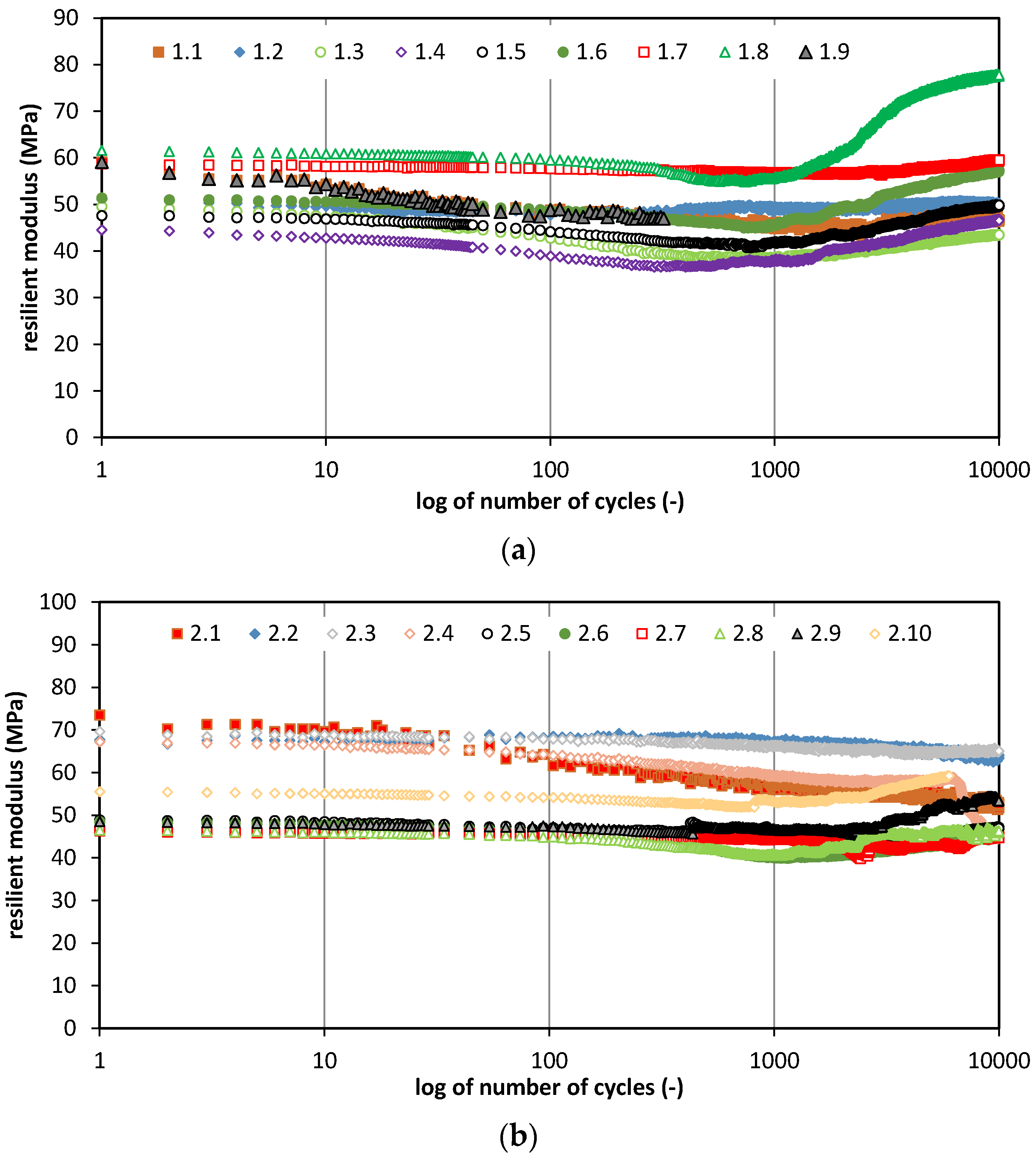
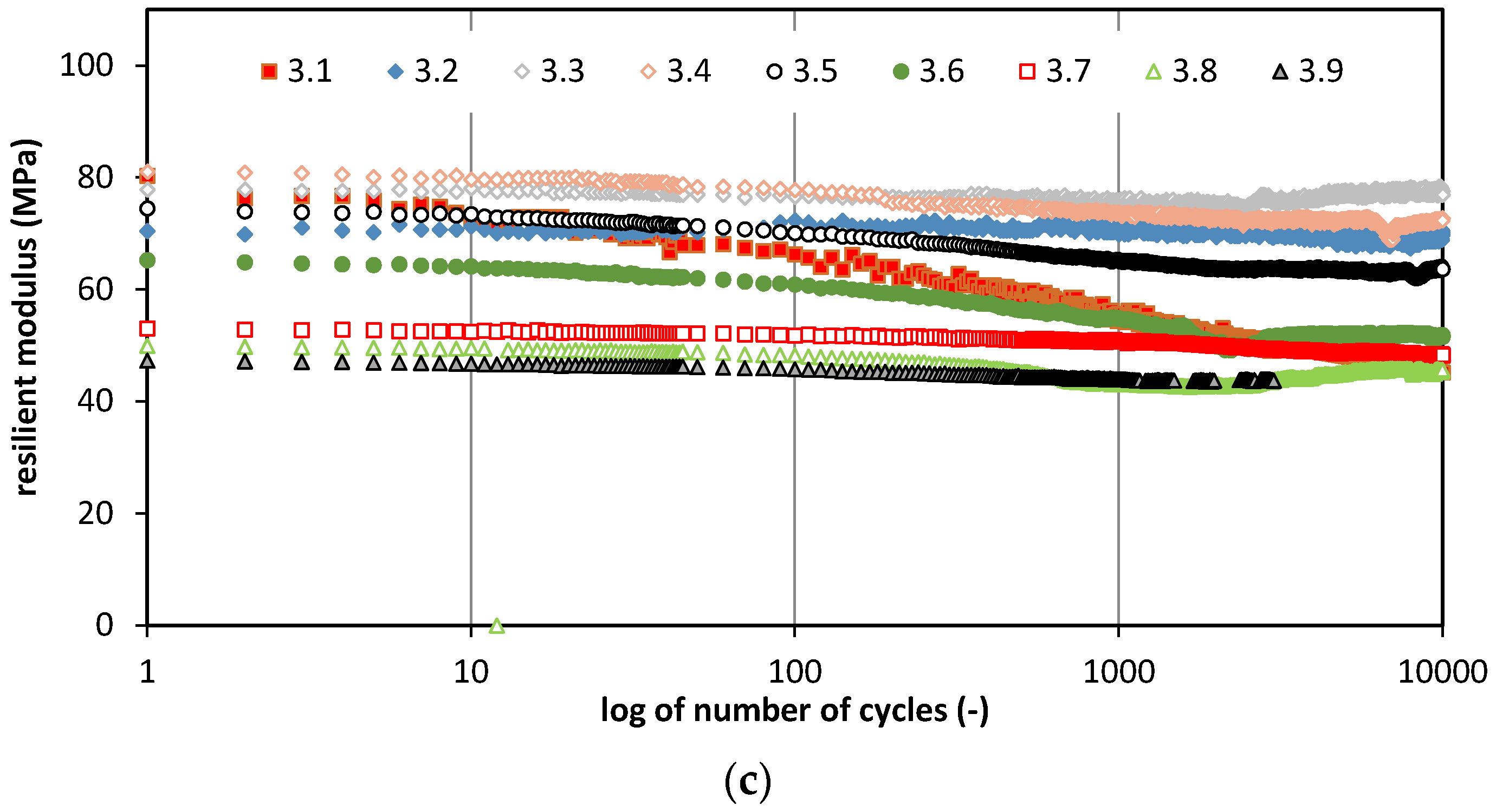
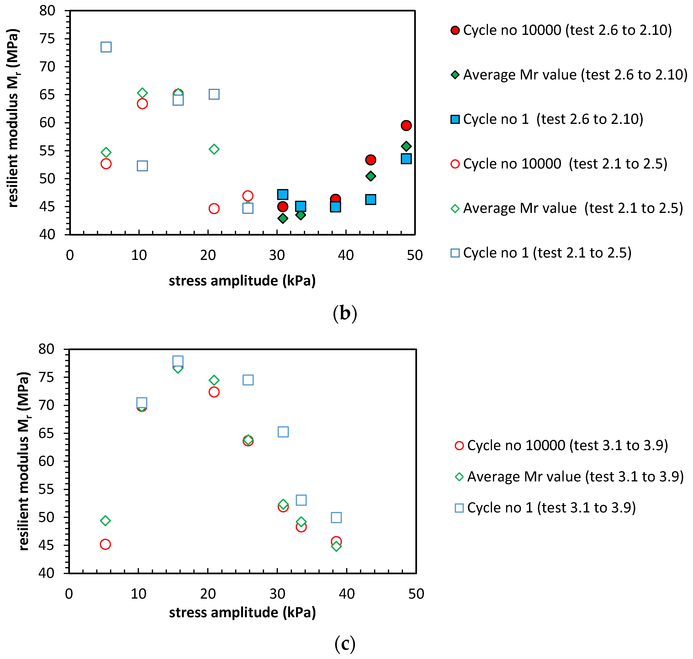
  • The recoverable strains characterized by the resilient modulus Mr value in the first cycle was between 44 and 59 MPa for confining pressure σ’3 equal to 45 kPa, between 48 and 78 MPa for σ’3 equal to 90 kPa, and from 44 to 81 MPa for σ’3 equal to 135 kPa. The resilient modulus Mr decrease was caused by plastic strain development.
  • The analytical model presented in this article takes into consideration the actual values of effective stress p′ (parameter T), actual excess pore water pressure in reference to initial conditions before cyclic loading Δu1, the loading characteristics (qmax and χ), and the position of the effective stress path (the T parameter).
  • The maximum resilient modulus for soil material was characterized. During cyclic loading, soil first degrades, then when Mr max reaches the plateau stage by around 1 × 10³ to 2 × 10³ cycles, pore pressure reaches equilibrium, and the maximal resilient modulus value starts to increase.

Author Contributions

Wojciech Sas and Andrzej Głuchowski prepared the manuscript and performed the cyclic triaxial tests. Emil Soból and Katrzyna Gabryś performed the TS tests. Katarzyna Gabryś and Alojzy Szymański consulted the research program and proofread the manuscript.

Conflicts of Interest

The authors declare no conflict of interest.

References

  1. Habiballah, T.; Chazallon, C. An elastoplastic model based on the shakedown concept for flexible pavements unboung granular materials. Int. J. Numer. Anal. Methods Geomech. 2005, 29, 577–596. [Google Scholar] [CrossRef]
  2. Sun, L.; Gu, C.; Wang, P. Effects of cyclic confining pressure on the deformation characteristics of natural soft clay. Soil Dyn. Earthq. Eng. 2015, 78, 99–109. [Google Scholar] [CrossRef]
  3. Zhou, J.; Gong, X.-N. Strain degradation of saturated clay under cyclic loading. Can. Geotech. J. 2001, 38, 208–212. [Google Scholar] [CrossRef]
  4. Macijauskas, D.; Van Baars, S. A 3D shear material damping model for man-made vibrations of the ground. In Proceedings of the 13th Baltic Sea Geotechnical Conference, Vilnius, Lithuania, 22–24 September 2016; pp. 159–165. [Google Scholar]
  5. Guo, L.; Wang, J.; Cai, Y.; Liu, H.; Gao, Y.; Sun, H. Undrained deformation behavior of saturated soft clay under long-term cyclic loading. Soil Dyn. Earthq. Eng. 2013, 50, 28–37. [Google Scholar] [CrossRef]
  6. Chai, J.C.; Miura, N. Traffic-load-induced permanent deformation of road on subsoil. J. Mech. Geoenviron. Eng. 2002, 128, 907–916. [Google Scholar] [CrossRef]
  7. Sas, W.; Głuchowski, A. Effects of stabilization with cement on mechanical properties of cohesive soil-sandy-silty clay. Ann. Wars. Univ. Life Sci. SGGW Land Reclam. 2012, 45, 193–205. [Google Scholar] [CrossRef]
  8. Fall, M.; Sawangsuriya, A.; Benson, C.H.; Edil, T.B.; Bosscher, P.J. On the investigations of resilient modulus of residual tropical gravel lateritic soils from Senegal (West Africa). Geotech. Geol. Eng. 2008, 26, 13–35. [Google Scholar] [CrossRef]
  9. Chen, H.H.; Marshek, K.M.; Saraf, C.L. Effects of truck tire contact pressure distribution on the design of flexible pavements: A three-dimensional finite element approach. Transp. Res. Rec. 1986, 1095, 72–78. [Google Scholar]
  10. Brown, S.F. 36th Rankine lecture: Soil mechanics in pavement engineering. Geotechnique 1996, 46, 383–426. [Google Scholar] [CrossRef]
  11. García-Rojo, R.; Herrmann, H.J. Shakedown of unbound granular material. Granul. Matter 2005, 7, 109–118. [Google Scholar] [CrossRef]
  12. Głuchowski, A.; Sas, W.; Bąkowski, J.; Szymański, A. Obciążenia cykliczne gruntu spoistego w warunkach bez odpływu. Acta Sci. Pol. Ser. Arch. 2016, 15, 57–77. [Google Scholar]
  13. Ghadimi, B.; Nega, A.; Nikraz, H. Simulation of shakedown behavior in pavement’s granular layer. Int. J. Eng. Technol. 2015, 7, 198–203. [Google Scholar] [CrossRef]
  14. Bassani, M.; Khosravifar, S.; Goulias, D.G.; Schwartz, C.W. Long-term resilient and permanent deformation behaviour of Controlled Low-Strength Materials for pavement applications. Transp. Geotech. 2015, 2, 108–118. [Google Scholar] [CrossRef]
  15. Hardy, M.S.A.; Cebon, D. Response of continuous pavements to moving dynamic loads. J. Eng. Mech. 1993, 119, 1762–1780. [Google Scholar] [CrossRef]
  16. Kiersnowska, A.; Koda, E.; Fabianowski, W.; Kawalec, J. Effect of the Impact of Chemical and Environmental Factors on the Durability of the High Density Polyethylene (HDPE) Geogrid in a Sanitary Landfill. Appl. Sci. 2017, 7, 22. [Google Scholar] [CrossRef]
  17. Koda, E.; Szymański, A.; Wolski, W. Field and laboratory experience with the use of strip drains in organic soils. Can. Geotech. J. 1993, 30, 308–318. [Google Scholar] [CrossRef]
  18. Huhtala, M. COST 337—Unbound granular materials for road pavement. In Proceedings of the 6th International Conference on the Bearing Capacity of Roads and Airfields, Lisbon, Portugal, 24–26 June 2002; Correia, A.G., Branco, F.E., Eds.; ARRB Group Limited: Lisbon, Portugal, 2002. [Google Scholar]
  19. Andrei, D.; Witczak, M.; Schwartz, C.; Uzan, J. Harmonized resilient modulus test method for unbound pavement materials. Transp. Res. Rec. 2004, 1874, 29–37. [Google Scholar] [CrossRef]
  20. Lytton, R.L.; Uzan, J.; Fernando, E.G.; Roque, R.; Hiltunen, D.R.; Stoffels, S.M. Development and Validation of Performance Prediction Models and Specifications for Asphalt Binders and Paving Mixtures; Report No. SHRP-A-357, Transportation Research Board 1993; National Research Council: Washington, DC, USA, 1993. [Google Scholar]
  21. Witczak, M.W.; Uzan, J. The Universal Airport Pavement Design System; Report I of V: Granular Material Characterization; Department of Civil Engineering, University of Maryland: College Park, MD, USA, 1998. [Google Scholar]
  22. Wang, J.; Guo, L.; Cai, Y.; Xu, C.; Gu, C. Strain and pore pressure development on soft marine clay in triaxial tests with a large number of cycles. Ocean Eng. 2013, 74, 125–132. [Google Scholar] [CrossRef]
  23. Massarsch, K.R. Deformation properties of fine-grained soils from seismic tests. Keynote lecture. Presented at the International Conference on Site Characterization, ISC’2, Porto, Portugal, 19–22 September 2004. [Google Scholar]
  24. Sas, W.; Gabryś, K. Laboratory measurement of shear stiffness in resonant column apparatus. Acta Sci. Pol. Ser. Arch. 2012, 12, 39–50. [Google Scholar]
  25. Atkinson, J.H.; Sallfors, G. Exerimental determination of stress-strain-time characteristics in laboratory and in situ tests. In Proceedings of the Xth International Conference on Soil Mechanics and Foundation Engineering, Florence, Italy, 27–30 May 1991; Volume 3, pp. 915–956. [Google Scholar]
  26. Lai, C.G.; Rix, G.J. Solution of the rayleigh eigenproblem in viscoelastic materials. Bull. Seismol. Soc. Am. 2002, 92, 2297–2309. [Google Scholar] [CrossRef]
  27. Sas, W.; Głuchowski, A.; Gabryś, K.; Soból, E.; Szymański, A. Studies on Cyclic and Dynamic Loading on Cohesive Soil in Road Engineering. In Proceedings of the 13th Baltic Sea Geotechnical Conference, Vilnius, Lithuania, 22–24 September 2016; pp. 85–92. [Google Scholar]
  28. Davich, P.; Labuz, J.; Guzina, B.; Drescher, A. Small Strain and Resilient Modulus Testing of Granular Soils; A Final Report No. 2004-39; Minnesota Department of Transportation: Saint Paul, MN, USA, 2004. [Google Scholar]
  29. Ba, M.; Tinjum, J.M.; Fall, M. Prediction of permanent deformation model parameters of unbound base course aggregates under repeated loading. Road Mater. Pavement Des. 2015, 16, 854–869. [Google Scholar] [CrossRef]
  30. Lavasani, M.; Namin, M.L.; Fartash, H. Experimental investigation on mineral and organic fibers effect on resilient modulus and dynamic creep of stone matrix asphalt and continuous graded mixtures in three temperature levels. Constr. Build. Mater. 2015, 95, 232–242. [Google Scholar] [CrossRef]
  31. Huang, Y.H. Pavement Analysis and Design, 2nd ed.; Pearson Prentice Hall: Bergen County, NJ, USA, 2008. [Google Scholar]
  32. Sas, W.; Głuchowski, A.; Gabryś, K.; Soból, E.; Szymański, A. Deformation Behavior of Recycled Concrete Aggregate during Cyclic and Dynamic Loading Laboratory Tests. Materials 2016, 9, 780. [Google Scholar] [CrossRef]
  33. Mehrotra, A.; Abu-Farsakh, M.; Gaspard, K. Development of subgrade Mr constitutive models based on physical soil properties. Road Mater. Pavement Des. 2016, 17, 4. [Google Scholar] [CrossRef]
  34. Guo, L.; Chen, J.; Wang, J.; Cai, Y.; Deng, P. Influences of stress magnitude and loading frequency on cyclic behavior of K0-consolidated marine clay involving principal stress rotation. Soil Dyn. Earthq. Eng. 2016, 84, 94–107. [Google Scholar] [CrossRef]
  35. Seed, H.B.; Chan, C.K.; Monismith, C.L. Effects of repeated loading on the strength and deformation of compacted clay. Highw. Res. Board Proc. 1955, 34, 541–558. [Google Scholar]
  36. Han, Z.; Vanapalli, S.K. State-of-the-Art: Prediction of resilient modulus of unsaturated subgrade soils. Int. J. Geomech. 2016, 16, 04015104. [Google Scholar] [CrossRef]
  37. Tang, Y.Q.; Cui, Z.Q.; Zhang, X.; Zhao, S.K. Dynamic response and pore pressure model of the saturated soft clay around the tunnel under vibration loading of Shanghai subway. Eng. Geol. 2008, 98, 126–132. [Google Scholar] [CrossRef]
  38. Cai, Y.; Gu, C.; Wang, J.; Juang, C.H.; Xu, C.; Hu, X. One-way cyclic triaxial behavior of saturated clay: Comparison between constant and variable confining pressure. J. Geotech. Geoenviron. Eng. 2012, 139, 797–809. [Google Scholar] [CrossRef]
  39. Ba, M.; Fall, M.; Sall, O.; Samb, F. Effect of compaction moisture content on the resilient modulus of unbound aggregates from Senegal (West Africa). Geomaterials 2012, 2, 19–23. [Google Scholar] [CrossRef]
  40. Hopkins, T.C.; Beckham, T.L.; Sun, C. Resilient Modulus of Compacted Crushed Stone Aggregate Bases; Research Report KTC-05-27/SPR-229-01-1F; Transportation Center, College of Engineering, University of Kentucky: Lexington, KY, USA, 2007. [Google Scholar]
  41. Uzan, J. Permanent deformation in flexible pavements. J. Transp. Eng. 2004, 130, 6–13. [Google Scholar] [CrossRef]
  42. Yaghoubi, E.; Disfani, M.M.; Arulrajah, A.; Kodikara, J. Impact of Compaction Methods on Resilient Response of Unsaturated Granular Pavement Material. Procedia Eng. 2016, 143, 323–330. [Google Scholar] [CrossRef]
  43. Hicks, R.G.; Monismith, C.L. Factors influencing the resilient properties of granular materials. Highw. Res. Rec. 1971, 345, 15–31. [Google Scholar]
  44. Assimaki, D.; Kausel, E.; Whittle, A. Model for dynamic shear modulus and damping for granular soils. J. Geotech. Geoenviron. Eng. 2000, 126, 859–869. [Google Scholar] [CrossRef]
  45. Polish Committee for Standardization. Eurokod 7 Projektowanie Geotechniczne Część 2: Rozpoznawanie i Badanie Podłoża Gruntowego; PN-EN 14688-2:2004; Polish Committee for Standardization: Warsaw, Poland, 2004. [Google Scholar]
  46. Polish Committee for Standardization. Badania Geotechniczne-Badania Laboratoryjne Gruntów-Część 4: Oznaczanie Składu Granulometrycznego; Standards PKN-CEN ISO/TS 17892-4:2009; Polish Committee for Standardization: Warsaw, Poland, 2009. [Google Scholar]
  47. American Association of State Highway and Transportation Officials. Standard Method of Test for Moisture-Density Relations of Soils Using a 2.5-kg (5.5-lb) Rammer and a 305-mm (12-in.) Drop; AASHTO T99; American Association of State Highway and Transportation Officials: Washington, DC, USA, 2015. [Google Scholar]
  48. Sas, W.; Szymański, A.; Gabryś, K. The behaviour of natural cohesive soils under dynamic excitations. In Proceedings of the 18th International Conference on Soil Mechanics and Geotechnical Engineering, Paris, France, 2–6 September 2013; Volume 2, pp. 1587–1590. [Google Scholar]
  49. Gabryś, K.; Sas, W.; Szymański, A. Kolumna rezonansowa jako urządzenie do badań dynamicznych gruntów spoistych. Przegląd Naukowy Inżynieria i Kształtowanie Środowiska 2013, 22, 3–15. [Google Scholar]
  50. Sas, W.; Gabryś, K.; Soból, E.; Szymański, A. Dynamic Characterization of Cohesive Material Based on Wave Velocity Measurements. Appl. Sci. 2016, 6, 49. [Google Scholar] [CrossRef]
  51. Wichtmann, T.; Niemunis, A.; Triantafyllidis, T. Strain accumulation in sand due to cyclic loading: Drained triaxial tests. Soil Dyn. Earthq. Eng. 2005, 25, 967–979. [Google Scholar] [CrossRef]
Figure 1. Diagram of differences between the elastic moduli in a small-strain zone and the resilient modulus in a plastic zone.
Applsci 07 00370 g001
Figure 2. Particle size distribution of the tested soil.
Applsci 07 00370 g002
Figure 3. Axial strain ε1 development during cyclic triaxial test for tests under (a) confining pressure σ’3 equal to 45 kPa; (b) for tests under σ’3 equal to 90 kPa; and (c) for tests under σ’3 equal to 135 kPa.
Applsci 07 00370 g003aApplsci 07 00370 g003b
Figure 4. Stress paths for different test conditions: radial stress equal to σ’3 (a) 45 kPa; (b) 90 kPa; and (c) 135 kPa, as defined in Table 2.
Applsci 07 00370 g004
Figure 5. Excess pore pressure generation during the three tests for radial stress versus axial strain ε1 for σ’3 (a) 45 kPa, (b) 90 kPa, (c) 135 kPa and versus the number of cycles for σ’3 (d) 45 kPa, (e) 90 kPa, and (f) 135 kPa.
Applsci 07 00370 g005
Figure 6. Young modulus Emax versus shear strain amplitude for isotropically-consolidated sandy clay (σ3 = 45 kPa and σ3 = 90 kPa); RCA—resonant column test; TS—torsional shear test for a frequency of 1 Hz.
Applsci 07 00370 g006
Figure 7. Schema of the hysteresis loop for Mr and Mr max calculations.
Applsci 07 00370 g007
Figure 8. Resilient modulus value of tested sandy clay for different conditions: radial stress σ’3 equal to (a) 45 kPa; (b) 90 kPa; and (c) 135 kPa, as defined in Table 2.
Applsci 07 00370 g008aApplsci 07 00370 g008b
Figure 9. Resilient modulus value of tested sandy clay for first and last cycles, and average value in the radial stress σ’3 equal to (a) 45 kPa, (b) 90 kPa and (c) 135 kPa, as defined in Table 2.
Applsci 07 00370 g009aApplsci 07 00370 g009b
Figure 10. Resilient modulus versus the number of cycles and analytical model T parameter for test results in 3D plots for isotropically-consolidated sandy clay (a) σ3 = 45 kPa; (b) σ3 = 90 kPa; and (c) σ3 = 135 kPa.
Applsci 07 00370 g010
Figure 11. Resilient modulus calculated by the proposed analytical model (blue points) and by the Uzan-Witczak model (red points) versus the resilient modulus value from tests (a) σ3 = 45 kPa; (b) σ3 = 90 kPa; and (c) σ3 = 135 kPa.
Applsci 07 00370 g011
Figure 12. Modulus value versus axial strain of tested sandy clay for different conditions: radial stress σ’3 equal to (a) 45 kPa and (b) 90 kPa, as defined in Table 2.
Applsci 07 00370 g012
Table 1. Physical and mechanical properties of sandy clay in this study.
PropertiesSymbolValue
Skeleton densityρs (g∙m−3)2.64
Volume densityρd (g∙m−3)2.09
Natural moisturewn (%)12.82
Liquid limitLL (%)18.9
Plasticity limitPL (%)10.3
Plasticity indexPI (-)8.6
Void ratioe0 (-)0.41
Optimum moisture contentWopt (%)10.2
Maximum dry unit densityγd max (g/cm3)2.09
Table 2. The stress parameters of cyclic triaxial test experiment for the tested sandy clay.
Captionσ3 (kPa)Δq (kPa)qm (kPa)qmin (kPa)qmax (kPa)qa (kPa)
Test 1.14510.6047.9021.3031.905.30
Test 1.24521.2053.2021.3042.5010.60
Test 1.34531.4058.7021.5052.9015.70
Test 1.44541.7064.4521.8063.5020.85
Test 1.54552.1070.2522.1074.2026.05
Test 1.64561.9075.5522.3084.2030.95
Test 1.74567.5078.3522.3089.8033.75
Test 1.84577.9083.5522.30100.2038.95
Test 1.94588.7088.7522.20110.9044.35
Test 2.19010.5047.4521.1031.605.25
Test 2.29021.0052.7021.1042.1010.50
Test 2.39031.4058.3021.3052.7015.70
Test 2.49041.8063.7021.4063.2020.90
Test 2.59051.6069.0021.6073.2025.80
Test 2.69061.7074.4521.8083.5030.85
Test 2.79066.9077.6522.1089.0033.45
Test 2.89077.0083.1022.3099.3038.50
Test 2.99087.2088.4022.40109.6043.60
Test 2.109097.5093.9522.60120.1048.75
Test 3.113510.5047.4521.1031.605.25
Test 3.213521.0052.7021.1042.1010.50
Test 3.313531.4058.3021.3052.7015.70
Test 3.413541.8063.7021.4063.2020.90
Test 3.513551.6069.0021.6073.2025.80
Test 3.613561.7074.4521.8083.5030.85
Test 3.713566.9077.6522.1089.0033.45
Test 3.813577.0083.1022.3099.3038.50
Test 3.913597.5093.9522.60120.1048.75
Table 3. The stress parameters of cyclic.
Average ValueStandard DeviationVarianceMax ValueMin Value
Dry soil mass (g)1092.019.8392.31121.11067.6
Height (cm)13.920.1250.01614.0313.76
Diameter (cm)6.920.0510.0036.986.86
Porosity (–)0.220.0050.0000.230.21
Water mass (g)112.284.70722.155119.60106.70
Full saturation soil mass (g)1204.2524.178584.5581240.801174.30
Soil dry density (g)2.090.0030.0002.092.08
Moisture (%)0.100.0030.0000.110.10

