Theory of Regions for Control Synthesis without Computing Reachability Graph

Abstract

This paper addresses the design of Petri net (PN) supervisor using the theory of regions for forbidden state problem with a set of general mutual exclusion constraints. In fact, as any method of supervisory control based on reachability graph, the theory of regions suffers from a technical obstacle in control synthesis, which is the necessity of computing the graph at each iteration step. Moreover, based on the reachability graph, which may contain a large number of states, with respect to the structural size of the system, the computation of PN controllers becomes harder and even impossible. The main contribution of this paper, compared to previous works, is the development of a control synthesis method in order to decrease significantly the computation cost of the PN supervisor. Thus, based on PN properties and mathematical concepts, the proposed methodology provides an optimal PN supervisor for bounded Petri nets following the interpretation of the theory of regions. Finally, case studies are solved by CPLEX software to compare our new control policy with previous works which use the theory of regions for control synthesis.

1. Introduction

Petri nets (PNs) present an effective tool to model and analyze Discrete Event Systems [1]. They have compact structures and can be represented in the form of matrices. Indeed, PNs can be analyzed by linear algebras. They play an important role in addressing the deadlock problems and analyzing the behavior of flexible manufacturing system [2,3,4,5]; a flexible manufacturing system can be defined as a computer controlled production system capable of processing a variety of part types. The flexibility of the system gives manufacturing firms an advantage in a quickly changing manufacturing environment [6].

In the framework of PNs, several approaches, such as the theory of regions, have been conducted for synthesizing PN controllers. The objective is to determine a convenient set of places and arcs connecting them to the transitions that, once added to a given PN plant model, will prevent the whole system from reaching forbidden states This PN controller is a designed subpart of the PN added to the controlled model. The theory of regions (TR) was initially proposed by Badouel and Darondeau [7] to design a bounded PN from a given reachability graph. Indeed, the set of all possible markings reachable from the initial marking with their all possible firing transitions is denoted a reachability graph (RG) [1] A PN is said bounded if it is $\mathrm{k}$-bounded for $\mathrm{k}>0$, i.e., the number of tokens in all places of the PN does not exceed $\mathrm{k}$. Nevertheless, TR has been newly interpreted for control synthesis problem by Ghaffari et al. to calculate an optimal PN supervisor. This PN controller is capable of satisfying a given control specification [8,9]. Indeed, this theory can be presented by a linear system composed of three classes of conditions: the reachability conditions, the Marking/transition separation instances (MTSI) conditions and basic cycle equations. The resolution of this linear system leads to the design of a PN controller which is a set of control places.

However, the steps of generating and analyzing the reachability graph present difficult tasks that weigh down heavily on the process of calculating PN controllers. Moreover, the combinatorial explosion of states in the RG complicates the calculation of PN controllers. Since computing time costs money, the objective of this work is to apply the TR for supervisory control without computing the RG in order to ease the supervisor calculation and eventually reduce the production cost.

In an industrial context, different products can be performed at the same time which can increase the control constraints and incite the monitor to make the necessary adjustments in order to control the system and maximize the production with less time.

In fact, many studies have been conducted on reachability graph analysis which represents a significant technique for synthesizing optimal/near-optimal PN controllers [10,11,12,13]. In [13], a RG based method is developed to calculate an optimal PN supervisor with the fewest control places for FMS modeled by PN. The RG is divided into a live zone and deadlock zone. The states in live zone are legal ones for a Flexible manufacturing system (FMS), and those in deadlock zone are deadlock or will lead to deadlocks. In [10], a vector covering method is used to reduce the number of markings to consider in the synthesis of PN controllers. An optimal supervisor with the fewest control places can be designed by solving a Minimal number of control places problem (MCCP). The PN controller obtained is optimal and structurally minimal in terms of the number of control places. However, it has a limitation: the computational burden is extremely hard, mainly for large models.

In addition, in Zhao et al. [14], a new method for supervisory control is developed using a divide-and-conquer strategy. Compared with most of traditional global-conquer methods of Uzam and Zhou [15,16], the computational efficiency of PN supervisors is improved. Nevertheless, as the number of shared resources in uncontrolled systems has increased, too many subsystems should be disposed. Thereby, as the net system size becomes larger, the improvement of this divide-and-conquer method will be impeded.

Our new control policy is based on the researches addressed on the use of the theory of regions. Up until now, the TR is recognized as one of the powerful method for deadlock prevention and supervisory control policies for obtaining maximally permissive PN controllers [8,9] which bans the set of forbidden states MI; unlike a legal marking, any state that does not comply with a control constraint is a non-legal state in the graph and will be denoted a forbidden marking $\mathrm{M}\in \mathrm{MI}$. In fact, many research works sought to lower the computational burden of the theory of regions; in [17], the authors used the siphons-approach before using the TR to synthesize PN controllers. Besides, in [18], a new method is developed for deadlocks prevention to decrease the number of reachability conditions of TR in order to facilitate the supervisor calculation. Their experimental results seems to be the most effective approach in deadlock prevention policy compared with existing works of [15,19,20]. Unfortunately, the computation of RG and its analysis to determine the basic cycles and the legal/forbidden markings for this method are still heavy.

However, the methods able to apply the theory of regions for control synthesis without computing the reachability graph have not been investigated. This paper sheds new light on TR simplification by eliminating the RG calculation and avoiding the combinatorial explosion of states which is a meaningful step for RG-based method. In addition, this work is only focused on bounded PNs.

In our previous works [21,22,23,24,25], a new method of minimal cuts in RG is developed using the theory of regions. Through this approach, we have also minimized the computational cost of PN supervisor using the TR on specific areas of the graph and not on the whole RG. Nonetheless, the graph generation step and its analysis are inevitable.

Accordingly, to reduce the computational burden of the TR, the RG generation step should be abandoned. In fact, based on PN properties and mathematical theories, one can speed up the synthesis process of PN controller. Consequently, the criterion of computation time of PN controllers will be a key factor in the comparison of this work with the previous ones [8,23].

The rest of this paper is structured as follows. Section 2 depicts the background of the theory of regions and PN tools. Section 3 introduces the concept of our new methodology for control synthesis. Next, three case studies will be given in Section 4 in order to illustrate the contribution of the proposed approach. Section 5 presents the results of comparison with previous works. Finally, conclusions are drawn in the Section 6.

2. Background

A Petri net is a directed graph consisting of places, transitions and valued arcs connecting them. Formally, a PN is a bipartite graph $N=\left(T,P,Pre,Post\right)$. $P$ is a finite set of places. $T$ is a finite set of transitions [1]. $Pre:P\times T\to \mathbb{N}$ is the pre-incidence function that specify weighted arcs from $P$ to $T$. $\mathbb{N}$ is the set of nonnegative integers. In addition, $Post:P\times T\to \mathbb{N}$ is the post-incidence function that specify weighted arcs from $T$ to $P$. The transitions of a PN can be partitioned into two disjoint subsets: $T_u$ the set of uncontrollable transitions and $T_c$ the set of controllable transitions. Controllable transitions can be disabled by the PN controller, while uncontrollable transitions cannot. Let $p^{\left(t\right)}$ (respectively, ${}_{}{}^{\left(t\right)}p_{}^{}$) be the set of output transitions (respectively, input transitions) of the place $p$. A PN can be represented by the so-called incidence matrix $C$ defined as $C\left(p,t\right)=Post\left(p,t\right)-Pre\left(p,t\right)$. Let $t^{\left(p\right)}$ (respectively, ${}_{}{}^{\left(p\right)}t_{}^{}$) the set of output places (respectively, input places) of transition $\mathrm{t}$. Besides, let $\mathrm{G}\left(N,M_0\right)$ be the reachability graph constructed from the initial marking $M_0$ of a given PN. Ϻ represents the set of markings $M\in G\left(N,M_0\right)$. A transition $t\in T$ is enabled from a marking $M$ (denoted by $M[t>$) if and only if $\mathrm{M}\ge \mathrm{Pre}\left(.,\mathrm{t}\right)$ if an enabled transition $\mathrm{t}$ is fired, it leads to a new marking $M^{\prime }$ such that: $M^{\prime }=M+C\left(.,t\right)$. This can be denoted by $M[t>M^{\prime }$. A marking $M^{\prime }$ is accessible from a given marking $M$ if there exists a firing sequence $\sigma =t_1,t_2\dots t_n$ transforming $M$ into $M^{\prime }$. By firing a sequence $\mathsf{\sigma }$ any marking $M$ reachable from $M_0$ satisfies the following state equation of Petri nets:

$$M=M_0+C\overrightarrow{\mathsf{\sigma }}$$

(1)

$\overrightarrow{\mathsf{\sigma }}:T\to \mathbb{N}$ is a vector of nonnegative integers is the occurrence of transition ${\mathrm{t}}_{\mathrm{i}}$ in $\mathsf{\sigma }$.

Let $C$ be the incidence matrix of marked PN. $C\left(p_i,t_j\right)=w\left(t_j,p_i\right)$ if $t_j\in p_{}^{\left(t\right)}{}_i$, $C\left(p_i,t_j\right)=-w\left(p_i,t_j\right)$ if $t_j\in p_i^{\left(t\right)}$, else 0. Where $w:F\to \mathbb{N}$ is a valuation function of arcs. $F\subseteq \left(T\times P\right)\cup \left(P\times T\right)$: Finite set of arcs. A Petri net is k-bounded if the number of tokens in each place does not exceed k. If k = 1, then the PN is said safe. A PN is live if all transitions are live; a transition is said live if it can always be made enabled starting from any reachable marking. A PN is reversible if from any reachable state $M$ there is an enabled sequence to return to the initial marking $M_0$.

Let us consider a set of legal markings; such admissible states correspond to a set of general mutual exclusion constraints GMECs. A constraint $\left(\overrightarrow{w},K\right)$ defines a set of legal markings [26]:

$$M_{\left(\overrightarrow{w},k\right)}=\left\{M\in M|{\overrightarrow{w}}^{T}M\le K\right\}$$

(2)

A new type of control specification constraint based on sequence transitions is developed in our previous work. This method is called admissible paths constraints APC $\left(\overrightarrow{v},C\right)$ which defines a set of legal sequences of transitions [27]:

$$T_{\left(\overrightarrow{v},C\right)}=\{\sigma \in {\sigma }^{*} |{\overrightarrow{v}}^T\overrightarrow{\sigma }\le C\}$$

(3)

The theory of regions in control synthesis was proposed by Ghaffari et al. [8,9] using the properties of PN for adding a controller $P_c$ to the initial PN model. The PN controller is characterized by its initial marking $M_0\left(P_c\right)$ and incidence vector $C\left(P_c,.\right)$. The TR is expressed by a linear system composed of three classes of conditions:

• Reachability conditions:

  $$M\left(P_c\right)=M_0\left(P_c\right)+C\left(P_c,.\right){\overrightarrow{\Gamma }}_M\ge 0$$

  (4)

  ${\overrightarrow{\mathrm{\Gamma }}}_{\mathrm{M}}$: Is the path between $M_0$ and $M$.
• MTSI condition: $\left(M,t\right)\in \mathsf{\Omega }$. $\mathsf{\Omega }$ is the set of prohibited state transitions. The transition $t$ may lead to a forbidden marking $M^{\prime }\in \mathrm{MI}$. $\mathrm{MI}$ is the set of markings which do not comply with a GMEC:

  $$M^{\prime }\left(P_c\right)= M_0\left(P_c\right)+C\left(P_c,.\right){\overrightarrow{\Gamma }}_M+C\left(P_c,t\right)<0$$

  (5)
• Basic cycle equations:

  $${\displaystyle \sum }_{\mathrm{t}\in \mathrm{T}}C\left(P_c,t\right)·\overrightarrow{\mathsf{\sigma }}\left[t\right]=0,\forall \mathsf{\sigma }\in R$$

  (6)

  $\overrightarrow{\mathsf{\sigma }}\left[t\right]$ is the algebraic sum of occurrences of t in $\mathsf{\sigma }$, and R is the desired behavior of the controlled system.

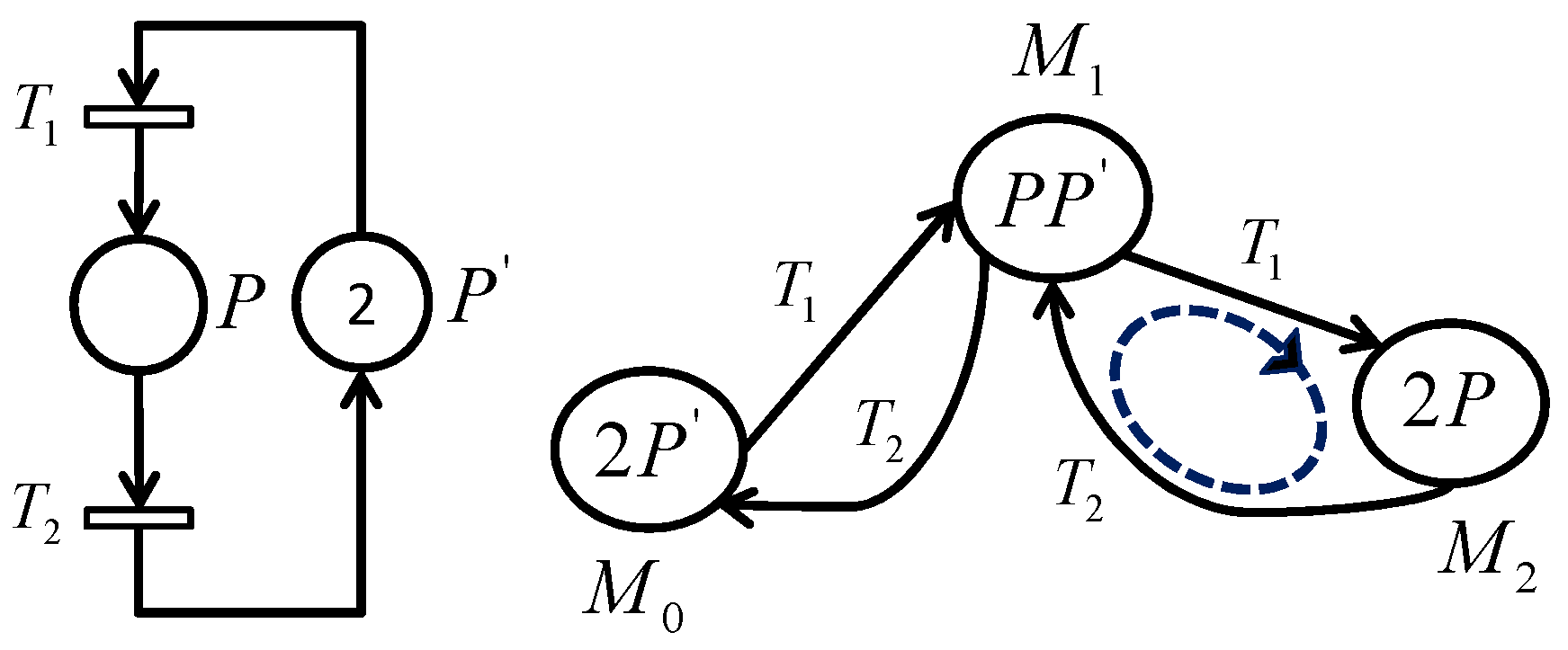
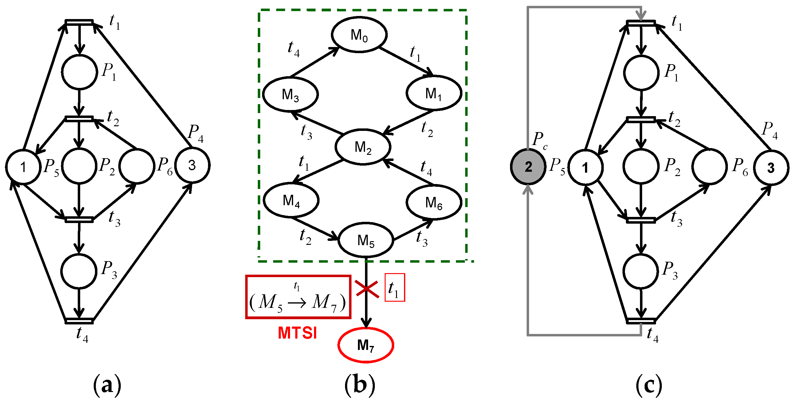
The application of the classical approach of the theory of regions [9] is given in the following example (i.e., see Figure 1). For a given PN (Figure 1a) [23], we firstly generate the reachability graph (Figure 1b). Next, one can analyze the RG to determine existing basic cycles, the legal markings and the forbidden ones (marking $M_7\in \mathrm{MI}$). The linear system of TR is given as follows:

$$M_0\left(P_c\right)\ge 0$$

$$M_1\left(P_c\right)=M_0\left(P_c\right)+C\left(P_c,t_1\right)\ge 0$$

$$M_2\left(P_c\right)=M_0\left(P_c\right)+C\left(P_c,t_1\right)+C\left(P_c,t_2\right)\ge 0$$

$$M_3\left(P_c\right)=M_0\left(P_c\right)+C\left(P_c,t_1\right)+C\left(P_c,t_2\right)+C\left(P_c,t_3\right)\ge 0$$

$$M_4\left(P_c\right)=M_0\left(P_c\right)+2C\left(P_c,t_1\right)+C\left(P_c,t_2\right)\ge 0$$

$$M_5\left(P_c\right)=M_0\left(P_c\right)+2C\left(P_c,t_1\right)+2C\left(P_c,t_2\right)\ge 0$$

$$M_6\left(P_c\right)=M_0\left(P_c\right)+2C\left(P_c,t_1\right)+2C\left(P_c,t_2\right)+C\left(P_c,t_3\right)\ge 0$$

$$M_7\left(P_c\right)=M_0\left(P_c\right)+2C\left(P_c,t_1\right)+2C\left(P_c,t_2\right)+C\left(P_c,t_1\right)<0$$

$$C\left(P_c,t_1\right)+C\left(P_c,t_2\right)+C\left(P_c,t_3\right)+C\left(P_c,t_4\right)=0$$

The resolution of this linear system generates the following PN controller $P_c:M_0\left(P_c\right)=2;$ $C\left(P_c,.\right)=\left(-1,0,0,1\right)$. The addition of this PN controller gives the controlled PN model shown in the Figure 1c.

In the following section, an effective method to avoid the combinatorial explosion of states in the presumed reachability graph will be introduced, where the generation step of RG is overlooked.

3. Design of PN Controller

3.1. Problem Setting

This work is focused on the minimization of the computational cost of the theory of regions by reducing the computation time for the synthesis of PN controllers. For this purpose, a new method based on PN tools and mathematical concepts, is proposed to design a PN supervisor without calculating the reachability graph.

Definition 1.

(Combinations without repetition) A k-combination without repetition of a set A with n elements is an arbitrary subset of A having k elements. If we take k objects among n without repetition and regardless of the appearance order, one can represent the k objects by a part of k-elements from a set with n elements. To determine the number of these provisions, one can determine the number of arrangements of k objects, and divide them by the number of provisions obtained from each other by a permutation: $\left(\begin{array}{c}n\\ k\end{array}\right)=\frac{A_k^n}{k!}=C_n^k$.

Definition 2.

(Combination with repetition) A k-combination with repetition of the set A is an arbitrary k-element multi-set of elements from A. If we take k objects among n without repetition and regardless of the appearance order, these objects can appear several times and we cannot represent them either with a part of k elements or with a k-tuple as their placement order is not involved. However, it is possible to represent such provisions with applications called combinations with repetition. The number of k-combinations with repetition of a set with n elements is denoted by ${Г}_n^k$ and formally: ${Г}_n^k=\left(\begin{array}{c}n+k-1\\ k\end{array}\right)$.

Definition 3.

(Usable sequence) A sequence is said to be a usable sequence if it leads to a reachable state that may exist in the presumed reachability graph. Let ${\sigma }_U$ be the set of usable sequences:

$${\mathsf{\sigma }}_{\mathrm{U}}=\left\{\mathsf{\sigma }\in {\mathsf{\sigma }}^{*}|{\mathrm{M}}_0[\mathsf{\sigma }>\mathrm{M},\mathrm{M}\in \mathrm{G}\left(\mathrm{N},{\mathrm{M}}_0\right)\right\}$$

(7)

Definition 4.

(Unusable sequence) A sequence is said to be an unusable sequence if it leads to a state that does not exist in the presumed reachability graph. Let ${\sigma }_{UN}$ be the set of unusable sequences:

$${\mathsf{\sigma }}_{\mathrm{UN}}=\left\{\mathsf{\sigma }\in {\mathsf{\sigma }}^{*}|{\mathrm{M}}_0[\mathsf{\sigma }>\mathrm{M},\mathrm{M}\notin \mathrm{G}\left(\mathrm{N},{\mathrm{M}}_0\right)\right\}$$

(8)

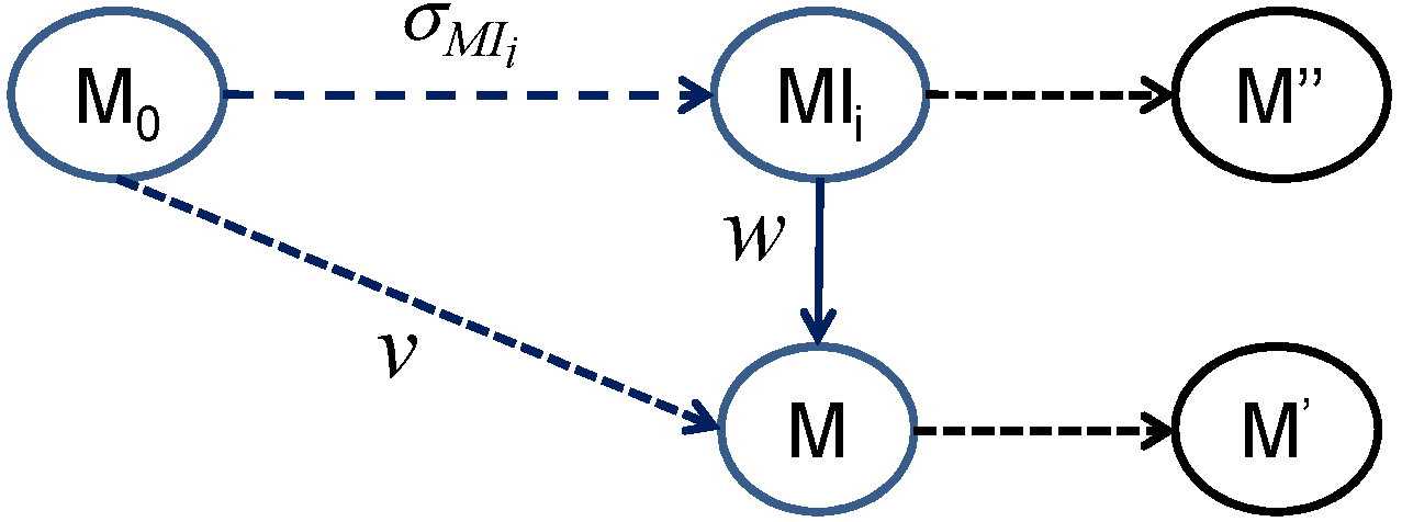
Definition 5.

(Prefix of a sequence) Let $MI$ be the set of forbidden markings that does not fulfill a given GMEC and let $E$ be the set of events. A firing sequence of a given forbidden marking ${\sigma }_{MI}{}_i$ is a prefix of a sequence $v\in E$, if there is another sequence $w$ such that $v={\sigma }_{MI}{}_{i}w$. That is, $v$ is the concatenation of ${\sigma }_{MI}{}_i$ and $w$ (see Figure 2). If $v$ is a physically possible sequence in the system, then naturally any prefix of $v$ is also a possible sequence in this system.

The key idea of the proposed method is to focus on the determination of the linear system of the theory of regions. Once the three classes of conditions of the TR, i.e., Equations (4)–(6), are defined, one can obtain the PN supervisor by adopting the interpretation of the theory of regions.

3.2. Basic Cycle Equations

Let $\mathrm{N}=\left(\mathrm{P},\mathrm{T},\mathrm{Pre},\mathrm{Post}\right)$ be a PN with its incidence matrix $\mathrm{C}$, and let ${\mathrm{X}}_{\mathrm{t}}$ be a nonnegative vector of n integers, solution of the equation $\mathrm{C}.{\mathrm{X}}_{\mathrm{t}}=0$. Let $\mathsf{\sigma }$ be the firing sequence for a legal marking $\mathrm{M}$ with $\mathsf{\sigma }={\mathrm{X}}_{\mathrm{t}}$. The sequence $\mathsf{\sigma }$ is called transition invariant [28]:

$$\mathrm{C}.\left[\begin{array}{c}{\mathrm{X}}_{\mathrm{t}1}\\ {\mathrm{X}}_{\mathrm{t}2}\\ .\\ .\\ {\mathrm{X}}_{\mathrm{tn}}\end{array}\right]=0$$

(9)

The resolution of this system generates the transition invariants that identify the basic cycle equations:

$${\displaystyle \sum }_{\mathrm{t}\in \mathrm{T}}\mathrm{C}\left({\mathrm{P}}_{\mathrm{c}},{\mathrm{t}}_{\mathrm{i}}\right).\overrightarrow{\mathsf{\sigma }}\left[\mathrm{t}\right]=0$$

(10)

Definition 6.

Let ${\tau }_{cycle}$ be the set of existing transitions in the basic cycle equations such that:

$${\mathsf{\tau }}_{\mathrm{cycle}}=\left\{\mathrm{t}\in \mathrm{T}|{\displaystyle \sum }_{\mathrm{t}\in \mathrm{T}}\mathrm{C}\left({\mathrm{P}}_{\mathrm{c}},\mathrm{t}\right).\overrightarrow{\mathsf{\sigma }}\left[\mathrm{t}\right]=0\right\}$$

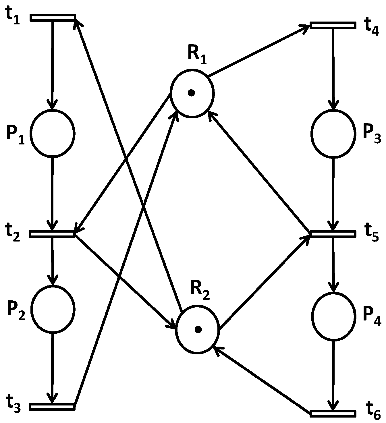
As shown in the example of PN given in Figure 3, the application of the transition invariant method generates the cycle equation of the theory of regions: $\mathrm{C}\left({\mathrm{P}}_{\mathrm{c}},{\mathrm{t}}_1\right)+\mathrm{C}\left({\mathrm{P}}_{\mathrm{c}},{\mathrm{t}}_2\right)=0$.

$$\mathrm{C}.{\mathrm{X}}_{\mathrm{t}}=0;\left[\begin{array}{cc}1& -1\\ -1& 1\end{array}\right]\left[\begin{array}{c}{\mathrm{x}}_{\mathrm{t}}\left({\mathrm{t}}_1\right)\\ {\mathrm{x}}_{\mathrm{t}}\left({\mathrm{t}}_2\right)\end{array}\right]=\left[\begin{array}{c}0\\ 0\end{array}\right]$$

$$\{\begin{array}{l}{\mathrm{x}}_{\mathrm{t}}\left({\mathrm{t}}_1\right)-{\mathrm{x}}_{\mathrm{t}}\left({\mathrm{t}}_2\right)=0\\ -{\mathrm{x}}_{\mathrm{t}}\left({\mathrm{t}}_1\right)+{\mathrm{x}}_{\mathrm{t}}\left({\mathrm{t}}_2\right)=0\end{array}\Rightarrow {\mathrm{X}}_{\mathrm{t}}{}^{\mathrm{T}}={\left[11\right]}^{\mathrm{T}}$$

Remark 1.

The determination of the reachability conditions/MTSI conditions is equivalent to the identification of paths connecting the initial marking $M_0$ and the legal/forbidden markings $M$. Thereby, to deduct this path, it is necessary to identify the corresponding sequence of transitions $\sigma$.

3.3. Reachability Conditions

Let ${\mathrm{P}}_{\mathrm{c}}$ be the control place to determine. Each marking $\mathrm{M}$ that satisfies a given GMEC must be reachable by the controlled PN model. As matter of fact, the reachability condition translates the state equation of Petri nets (1). The difference is that the equation is positively assigned and the reachable marking is legal:

$$\mathrm{M}\left({\mathrm{P}}_{\mathrm{c}}\right)={\mathrm{M}}_0\left({\mathrm{P}}_{\mathrm{c}}\right)+\mathrm{C}.\overrightarrow{{\mathsf{\sigma }}_{\mathrm{M}}}\ge 0$$

(11)

In order to determine all the firing sequences, the combinatorial analysis methods were introduced in our work (i.e., see Definitions 1 and 2).

Proposition 1.

For a safe PN, the set of firing sequences of transitions denoted by S corresponds mathematically to combinations without repetition where i transitions are chosen among ${\tau }_{cycle}$:

$$\left|\mathrm{S}\right|={\displaystyle \sum }_{\mathrm{i}=0}^{\mathrm{card}\left({\mathsf{\tau }}_{\mathrm{cycle}}\right)}{\mathrm{C}}_{\mathrm{card}\left({\mathsf{\tau }}_{\mathrm{cycle}}\right)}^{\mathrm{i}}$$

Proposition 2.

For a k-bounded PN with $k>1$, the set of firing sequences of transitions denoted by S corresponds mathematically to combinations with repetition where i transitions are chosen among ${\tau }_{cycle}$:

$$\left|\mathrm{S}\right|={\displaystyle \sum }_{\mathrm{i}=0}^{\mathrm{card}\left({\mathsf{\tau }}_{\mathrm{cycle}}\right)}{\mathsf{Г}}_{\mathrm{card}\left({\mathsf{\tau }}_{\mathrm{cycle}}\right)}^{\mathrm{i}}$$

A safe PN is a 1-bounded PN (k = 1). Each transition ${\mathrm{t}}_{\mathrm{i}}\in {\mathsf{\tau }}_{\mathrm{cycle}}$ is fired no more than once in a given sequence $\mathsf{\sigma }$. Similarly, ${\mathrm{C}}_{\mathrm{card}\left({\mathsf{\tau }}_{\mathrm{cycle}}\right)}^{\mathrm{i}}$ is a collection of i transitions among $\mathrm{card}\left({\mathsf{\tau }}_{\mathrm{cycle}}\right)$ and the transition can be collected at most once. Therefore, the sum of transition combinations $\sum _{\mathrm{i}=0}^{\mathrm{card}\left({\mathsf{\tau }}_{\mathrm{cycle}}\right)}{\mathrm{C}}_{\mathrm{card}\left({\mathsf{\tau }}_{\mathrm{cycle}}\right)}^{\mathrm{i}}=\frac{\mathrm{card}\left({\mathsf{\tau }}_{\mathrm{cycle}}\right)!}{\mathrm{i}!\left(\mathrm{card}\left({\mathsf{\tau }}_{\mathrm{cycle}}\right)-\mathrm{i}\right)!}$ corresponds to all firing sequences of transitions $(\sum _{\mathrm{i}=0}^{\mathrm{card}\left({\mathsf{\tau }}_{\mathrm{cycle}}\right)}{\mathsf{\sigma }}_{\mathrm{i}}=\mathrm{S}$).

3.4. MTSI Conditions

Up to here, the reachability conditions and the basic cycle equations are known. Furthermore, the initial marking of PN model is given. Through these data and our previous work, one can calculate the MTSI conditions.

Corollary 1.

If the control specification is expressed as GMEC $\left(\overrightarrow{w}, K\right)$, then the identification of the set of forbidden states MI is possible without generating reachability graph $G\left(N,M_0\right)$ using the canonic markings method [25].

Remark 2.

The firing sequences of transitions are generated from the set ${\tau }_{cycle}$ and not from $T$ since the cycle equations exist in the desired behavior of the controlled system and not in the whole graph $G\left(N,M_0\right)$.

Since the set MI of forbidden markings is known, one can determine the set of forbidden sequences ${\mathsf{\sigma }}_{\mathrm{MI}}$. Moreover, the calculation of ${\mathsf{\sigma }}_{\mathrm{MI}}$ can be done in two ways:

• Algebraic method: By using the state equation: $\mathrm{MI}={\mathrm{M}}_0+\mathrm{C}.{\mathsf{\sigma }}_{\mathrm{MI}}$
  If $\det \left(\mathrm{C}\right)\ne 0$, one can calculate the forbidden sequence ${\mathsf{\sigma }}_{\mathrm{MI}}$:

  $${\mathsf{\sigma }}_{\mathrm{MI}}=\left(\mathrm{MI}-{\mathrm{M}}_0\right).{\mathrm{C}}^{-1}$$
• Canonic markings method [24]: From the GMEC, one can synthesize the forbidden state that does not satisfy the control specification. However, by performing back chaining ${\mathrm{CH}}_{\mathrm{b}}$, one can find the initial marking ${\mathrm{M}}_0$:

  $${\mathrm{CH}}_{\mathrm{b}}={\displaystyle \sum }_{\mathrm{i}}{}_{}{}^{({\mathrm{t}}_{\mathrm{i}})}\mathrm{p}_{}^{}|\mathrm{p}\in {\mathrm{t}}_{\mathrm{i}}^{\left(\mathrm{p}\right)},\mathrm{M}\left(\mathrm{p}\right)\le {\mathsf{\beta }}_{\mathrm{i}}^{-}$$
  ${\mathsf{\beta }}_{\mathrm{i}}^{-}$: Is the weight for each fired transition during the back chaining.

Consequently, one can determine the MTSI condition:

$${\mathrm{M}}_0\left({\mathrm{P}}_{\mathrm{c}}\right)+\mathrm{C}.\overrightarrow{{\mathsf{\sigma }}_{{\mathrm{MI}}_{\mathrm{i}}}}<0$$

(12)

By summarizing, a new interpretation of the theory of regions is developed in this work to determine the linear system formed of Equations (10)–(12).

3.5. Filtering of Sequences S

The filtering step of sequences S is necessary in our work in order to specify the correct linear system of the theory of regions. Indeed, the generation of the set of sequences S with/without repetition gives unusable sequences ${\mathsf{\sigma }}_{\mathrm{UN}}$ and usable sequences ${\mathsf{\sigma }}_{\mathrm{U}}$ (i.e., see Definitions 3 and 4). Therefore, the usable sequences and the basic cycle equations allow us to accurately determine the linear system of the theory of regions.

The filtering of sequences S is performed using the state equation of Petri nets:

$${\mathrm{M}}_{\mathrm{x}}={\mathrm{M}}_0+\mathrm{C}.\overrightarrow{{\mathsf{\sigma }}_i}$$

where ${\mathrm{M}}_{\mathrm{x}}$ is the new marking to determine by testing all sequences of the set S.

Thus, the unusable sequences to reject are:

• Sequences having prefixes ${\mathsf{\sigma }}_{\mathrm{MI}}$ (i.e., see Definition 5);
• Sequences leading to null markings; and
• Sequences leading to negative markings (A negative marking is a vector containing at least one negative component).

The synthesis method of PN controllers using the new interpretation of the theory of regions is described in the following Algorithm 1.

Algorithm 1. Algorithm of the synthesis method
Given a PN with its initial marking ${\mathrm{M}}_0$ and the set of forbidden markings MI, let S be the set of firing transitions sequences.
(1)	Determine the basic cycle equations using the transitions invariants method and let ${\mathsf{\tau }}_{\mathrm{cycle}}$ be the set of transitions in cycle equations.
(2)	If the PN is safe, then determine S with $\left|\mathrm{S}\right|=\sum _{\mathrm{i}=0}^{\mathrm{card}\left({\mathsf{\tau }}_{\mathrm{cycle}}\right)}{\mathrm{C}}_{\mathrm{card}\left({\mathsf{\tau }}_{\mathrm{cycle}}\right)}^{\mathrm{i}}$ If the PN is k-bounded with k > 1, then determine S with $\left|\mathrm{S}\right|=\sum _{\mathrm{i}=0}^{\mathrm{card}\left({\mathsf{\tau }}_{\mathrm{cycle}}\right)}{\mathsf{Г}}_{\mathrm{card}\left({\mathsf{\tau }}_{\mathrm{cycle}}\right)}^{\mathrm{i}}$
(3)	Identify from S the set of forbidden firing sequences of transitions ${\mathsf{\sigma }}_{\mathrm{MI}}|{\mathrm{M}}_0[{\mathsf{\sigma }}_{\mathrm{MI}}>{\mathrm{M}}^{\text{'}},{\mathrm{M}}^{\text{'}}\in \mathrm{MI}$.
(4)	Filter the firing sequences of transitions S to get the set ${\mathsf{\sigma }}_{\mathrm{U}}$ of usable sequences
(5)	While ${\mathsf{\sigma }}_{\mathrm{MI}}\ne \varnothing$ do:
	(5.1)	For each forbidden sequences of transitions ${\mathsf{\sigma }}_{\mathrm{i}}\in {\mathsf{\sigma }}_{\mathrm{MI}}$, write the linear system of the theory of regions composed of: The MTSI condition of the eventual forbidden sequence ${\mathsf{\sigma }}_{\mathrm{i}}\in {\mathsf{\sigma }}_{\mathrm{MI}}$ The reachabiliy conditions of the remaining sequences ${\mathsf{\sigma }}_{\mathrm{U}}/{\mathsf{\sigma }}_{\mathrm{MI}}$ The basic cycle equations
	(5.2)	Solve the linear system of TR and let $\left({\mathrm{M}}_0\left({\mathrm{P}}_{\mathrm{ci}}\right);\mathrm{C}\left({\mathrm{P}}_{\mathrm{ci}},.\right)\right)$ be the solution sought.
(6)	Remove redundant control places to obtain the controlled Petri net.

In the first three steps, the cycle equations and the sequences S are generated. Thus, one can filter the firing sequences to form the linear system of the theory of regions by using only the usable sequences and the cycle equations. In the following steps, the theory of regions is applied and the PN supervisor is synthesized.

In the next section, three case studies are provided to show that the Algorithm 1 can find an optimal PN supervisor using the theory of regions without computing reachability graph.

4. Case Studies

In this section, three case studies of bounded PNs are solved using CPLEX software with a C program to evaluate our control policy. Notably, the three cases include two subclasses of PN (i.e., safe PNs and k-bounded PNs with k > 0) in order to apply and test the propositions of Section 3.3. Owing to the limitation of paper space, the reachability conditions are not listed in these case studies.

Indeed, in Example 1, the resources are shared and the PN is safe which allow us to calculate the firing sequences using combinations without repetition (i.e., Proposition 1). Then, we can better assess the effectiveness of our method since safe PNs are special cases of PNs.

Next, Examples 2 and 3 model three stations of the FMS installed in our laboratory with k-bounded PNs. Consequently, the sequences of firing transitions will be determined employing combinations with repetition. In fact, Example 2 deals with two assembly stations with a production constraint, while Example 3 models a control quality station with another general mutual exclusion constraint. These two examples represent two real cases of production constraints, which allow us to tackle two real situations of industry.

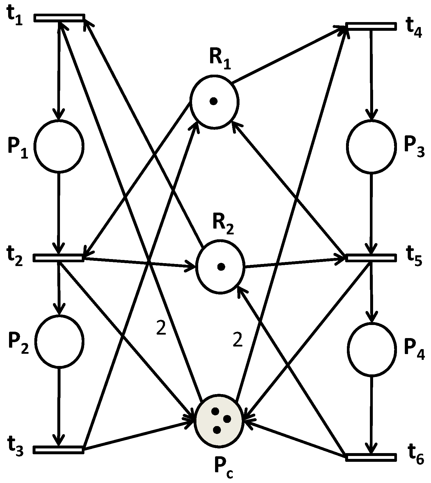
4.1. Case Study 1

This first case study addresses a PN model with two machines sharing two resources ${\mathrm{R}}_1$ and ${\mathrm{R}}_2$ shown in Figure 4. The places ${\mathrm{P}}_1$ and ${\mathrm{P}}_3$ materialize two operations. To deal with the organizational and synchronization problem between two processes in parallel which is a current problem, we have to satisfy the following control specification: $\mathrm{M}\left({\mathrm{P}}_1\right)+\mathrm{M}\left({\mathrm{P}}_3\right)\le 1$.

• Basic cycle equations:

The resolution of the equation: $\mathrm{C}.{\left[{\mathrm{x}}_1{\mathrm{x}}_2\dots {\mathrm{x}}_{\mathrm{n}}\right]}^{\mathrm{T}}=0$ gives the basic cycle Equation (10).

$$\mathrm{C}{.\mathrm{X}}_{\mathrm{t}}=\left[\begin{array}{cccccc}1& -1& 0& 0& 0& 0\\ 0& 1& -1& 0& 0& 0\\ 0& 0& 0& 1& -1& 0\\ 0& 0& 0& 0& 1& -1\\ 0& -1& 1& -1& 1& 0\\ -1& 1& 0& 0& -1& 1\end{array}\right]\left[\begin{array}{c}{\mathrm{x}}_{\mathrm{t}}{(\mathrm{t}}_1)\\ {\mathrm{x}}_{\mathrm{t}}{(\mathrm{t}}_2)\\ {\mathrm{x}}_{\mathrm{t}}{(\mathrm{t}}_3)\\ {\mathrm{x}}_{\mathrm{t}}{(\mathrm{t}}_4)\\ {\mathrm{x}}_{\mathrm{t}}{(\mathrm{t}}_5)\\ {\mathrm{x}}_{\mathrm{t}}{(\mathrm{t}}_6)\end{array}\right]=\left[\begin{array}{c}0\\ 0\\ 0\\ 0\\ 0\\ 0\end{array}\right]$$

$$\{\begin{array}{l}{\mathrm{x}}_{\mathrm{t}}\left({\mathrm{t}}_1\right)-{\mathrm{x}}_{\mathrm{t}}\left({\mathrm{t}}_2\right)=0\\ {\mathrm{x}}_{\mathrm{t}}\left({\mathrm{t}}_2\right)-{\mathrm{x}}_{\mathrm{t}}\left({\mathrm{t}}_3\right)=0\\ {\mathrm{x}}_{\mathrm{t}}\left({\mathrm{t}}_4\right)-{\mathrm{x}}_{\mathrm{t}}\left({\mathrm{t}}_5\right)=0\\ {\mathrm{x}}_{\mathrm{t}}\left({\mathrm{t}}_5\right)-{\mathrm{x}}_{\mathrm{t}}\left({\mathrm{t}}_6\right)=0\\ -{\mathrm{x}}_{\mathrm{t}}\left({\mathrm{t}}_2\right)+{\mathrm{x}}_{\mathrm{t}}\left({\mathrm{t}}_3\right)-{\mathrm{x}}_{\mathrm{t}}\left({\mathrm{t}}_4\right)+{\mathrm{x}}_{\mathrm{t}}\left({\mathrm{t}}_5\right)=0\\ -{\mathrm{x}}_{\mathrm{t}}\left({\mathrm{t}}_1\right)+{\mathrm{x}}_{\mathrm{t}}\left({\mathrm{t}}_2\right)-{\mathrm{x}}_{\mathrm{t}}\left({\mathrm{t}}_5\right)+{\mathrm{x}}_{\mathrm{t}}\left({\mathrm{t}}_6\right)=0\end{array}\Rightarrow \begin{array}{c}{{(\mathrm{X}}_{\mathrm{t}}^1)}^{\mathrm{T}}=[000111]\\ {{(\mathrm{X}}_{\mathrm{t}}^2)}^{\mathrm{T}}=[111000]\end{array}$$

The corresponding sequences of the basic cycle equations are: ${\mathsf{\sigma }}_1=\left({\mathrm{t}}_4{\mathrm{t}}_5{\mathrm{t}}_6\right)$ and ${\mathsf{\sigma }}_2=\left({\mathrm{t}}_1{\mathrm{t}}_2{\mathrm{t}}_3\right)$. Thus, the basic cycle Equation (10) can be listed as follows:

$$\mathrm{C}\left({\mathrm{P}}_{\mathrm{ci}},{\mathrm{t}}_4\right)+\mathrm{C}\left({\mathrm{P}}_{\mathrm{ci}},{\mathrm{t}}_5\right)+\mathrm{C}\left({\mathrm{P}}_{\mathrm{ci}},{\mathrm{t}}_6\right)=0$$

$$\mathrm{C}\left({\mathrm{P}}_{\mathrm{ci}},{\mathrm{t}}_1\right)+\mathrm{C}\left({\mathrm{P}}_{\mathrm{ci}},{\mathrm{t}}_2\right)+\mathrm{C}\left({\mathrm{P}}_{\mathrm{ci}},{\mathrm{t}}_3\right)=0$$

• Reachability conditions:

According to the Definition 6, the set ${\mathsf{\tau }}_{\mathrm{cycle}}$ contains six transitions, i.e., $\mathrm{card}\left({\mathsf{\tau }}_{\mathrm{cycle}}\right)=$ 6:

$${\mathsf{\tau }}_{\mathrm{cycle}}=\left\{{\mathrm{t}}_1,{\mathrm{t}}_2,{\mathrm{t}}_3,{\mathrm{t}}_4,{\mathrm{t}}_5,{\mathrm{t}}_6\right\}$$

The PN is safe (k = 1). Then, conforming to the Proposition 1 the set S of firing sequences of transitions is generated through combinations without repetition.

$$\left|\mathrm{S}\right|={\displaystyle \sum }_{\mathrm{i}=0}^{\mathrm{card}\left({\mathsf{\tau }}_{\mathrm{cycle}}\right)}{\mathrm{C}}_{\mathrm{card}\left({\mathsf{\tau }}_{\mathrm{cycle}}\right)}^{\mathrm{i}}={\displaystyle \sum }_{\mathrm{i}=0}^6{\mathrm{C}}_6^{\mathrm{i}}={\mathrm{C}}_6^0+{\mathrm{C}}_6^1+{\mathrm{C}}_6^2+{\mathrm{C}}_6^3+{\mathrm{C}}_6^4+{\mathrm{C}}_6^5+{\mathrm{C}}_6^6=64$$

Afterwards, the sequences S will be filtered conforming to the criteria mentioned in Section 3.4 in order to obtain the usable sequences listed in

Table 1. Usable sequences of Example 1.

Sequence No.	σ = (t1t2t3t4t5t6)
σ1	(0 0 0 0 0 0)
σ2	(1 0 0 0 0 0)
σ3	(0 0 0 1 0 0)
σ4	(1 1 0 0 0 0)
σ5	(0 0 0 1 1 0)
σ6	(0 0 0 2 1 0)
σ7	(2 1 0 0 0 0)
σ8	(1 0 0 1 0 0)

.

Finally, by identifying the usable sequences $\mathrm{card}\left({\mathsf{\sigma }}_{\mathrm{U}}\right)=$8, one can obtain the reachability conditions (11).

• MTSI conditions:

The set of forbidden markings that do not fulfill the control specification are listed in

Table 2. Forbidden markings (P1P3) of Example 1.

M(P1)	M(P3)
1	1

. In agreement with Corollary 1, the forbidden sequences σ_MI can be obtained using the canonic markings method and are listed in the

Table 3. Forbidden sequences of Example 1.

Sequence No.	σMIi = (t1t2t3t4t5t6)
${\mathsf{\sigma }}_{{\mathrm{MI}}_1}$	$\left(100100\right)$

. Then, the MTSI condition can be obtained as follows:

$${\mathrm{M}}_0\left({\mathrm{P}}_{\mathrm{c}}\right)+\mathrm{C}\left({\mathrm{P}}_{\mathrm{c}},{\mathrm{t}}_1\right)+\mathrm{C}\left({\mathrm{P}}_{\mathrm{c}},{\mathrm{t}}_4\right)<0$$

Furthermore, by applying our algorithm, there is one control place ${\mathrm{P}}_{\mathrm{c}}$ obtained when Equations (10)–(12) are solved. The PN controller information is listed in

Table 4. PN controllers of Example 1.

Additional Control Places	M0i(Pci)	C(Pci,.)
$P_c$	3	$\left(-2,1,1,-2,1,1\right)$

. Therefore, the controlled PN model is given in Figure 5.

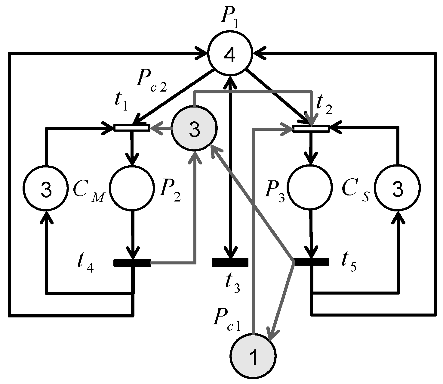
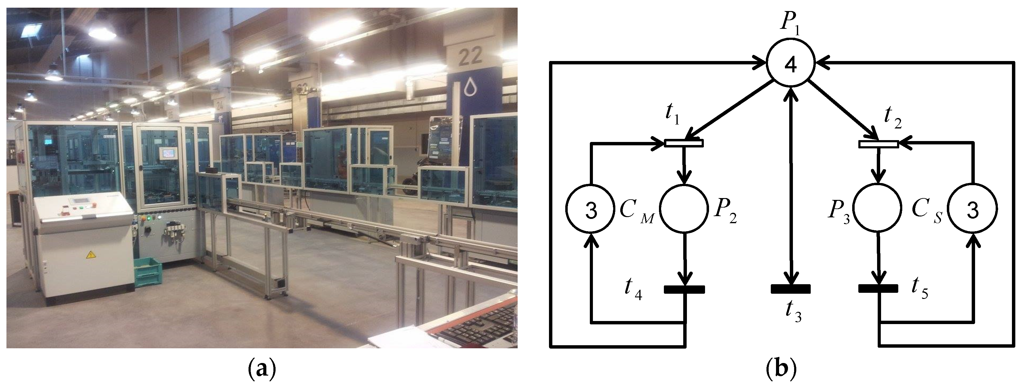
4.2. Case Study 2

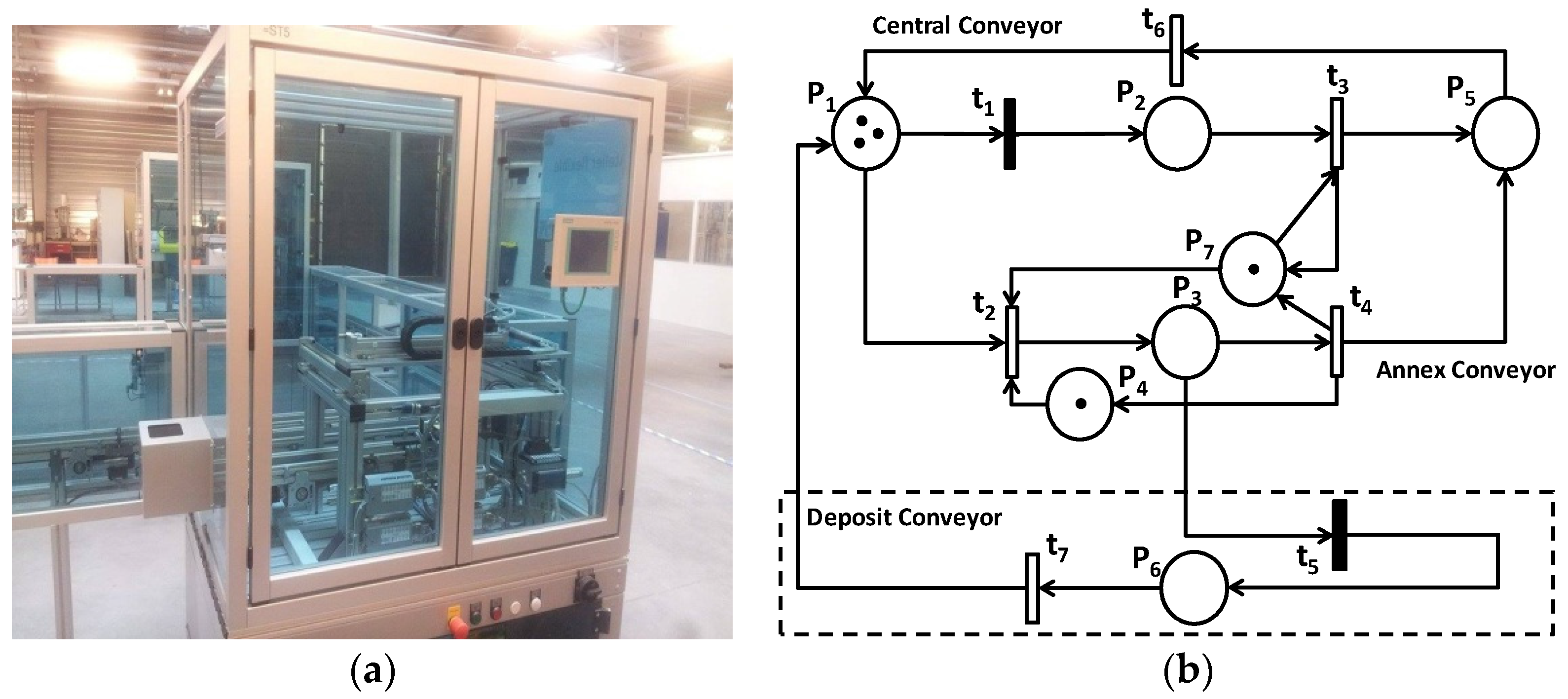
A flexible manufacturing system in the Lorraine University contains two assembly stations in which engraved glass pieces are assembled with stands. The physical system and the PN model are presented in Figure 6a,b. The place ${\mathrm{P}}_2$ models our production machine, while the place ${\mathrm{P}}_3$ represents a subcontractor production. The capacities of three pieces of the machine and the subcontractor are modeled by ${\mathrm{C}}_{\mathrm{M}}$ and ${\mathrm{C}}_{\mathrm{S}}$, respectively. In addition, the place ${\mathrm{P}}_1$ represents our stock production. Moreover, the entry and exit events of the pallets in annex conveyors are modeled by transitions $\left({\mathrm{t}}_1,{\mathrm{t}}_2\right)$ and $\left({\mathrm{t}}_4,{\mathrm{t}}_5\right)$, respectively. Alternatively, the pallet continues its way in the main conveyor by ${\mathrm{t}}_3$. Note that ${\mathrm{t}}_3,{\mathrm{t}}_4$ and ${\mathrm{t}}_5$ are uncontrollable.

The following scenario is employed: If ${\mathrm{P}}_3$ and ${\mathrm{P}}_2$ represent the subcontractor and the machine, the subcontractor production should be minimized to increase our profits. This control specification can be expressed by the following GMEC: $\mathrm{M}\left({\mathrm{P}}_2\right)+2\mathrm{M}\left({\mathrm{P}}_3\right)\le 3$.

• Basic cycle equations: $\mathrm{C}.{\left[{\mathrm{x}}_1{\mathrm{x}}_2\dots {\mathrm{x}}_{\mathrm{n}}\right]}^{\mathrm{T}}=0$

$$\mathrm{C}{.\mathrm{X}}_{\mathrm{t}}=\left[\begin{array}{ccccc}-1& -1& 0& 1& 1\\ 1& 0& 0& -1& 0\\ 0& 1& 0& 0& -1\\ -1& 0& 0& 1& 0\\ 0& -1& 0& 0& 1\end{array}\right]\left[\begin{array}{l}{\mathrm{x}}_{\mathrm{t}}\left({\mathrm{t}}_1\right)\\ {\mathrm{x}}_{\mathrm{t}}\left({\mathrm{t}}_2\right)\\ {\mathrm{x}}_{\mathrm{t}}\left({\mathrm{t}}_3\right)\\ {\mathrm{x}}_{\mathrm{t}}\left({\mathrm{t}}_4\right)\\ {\mathrm{x}}_{\mathrm{t}}\left({\mathrm{t}}_5\right)\end{array}\right]=\left[\begin{array}{l}0\\ 0\\ 0\\ 0\\ 0\end{array}\right]$$

$$\{\begin{array}{l}-{\mathrm{x}}_{\mathrm{t}}\left({\mathrm{t}}_1\right)-{\mathrm{x}}_{\mathrm{t}}\left({\mathrm{t}}_2\right)+{\mathrm{x}}_{\mathrm{t}}\left({\mathrm{t}}_4\right)+{\mathrm{x}}_{\mathrm{t}}\left({\mathrm{t}}_5\right)=0\\ {\mathrm{x}}_{\mathrm{t}}\left({\mathrm{t}}_1\right)-{\mathrm{x}}_{\mathrm{t}}\left({\mathrm{t}}_4\right)=0\\ {\mathrm{x}}_{\mathrm{t}}\left({\mathrm{t}}_2\right)-{\mathrm{x}}_{\mathrm{t}}\left({\mathrm{t}}_5\right)=0\\ -{\mathrm{x}}_{\mathrm{t}}\left({\mathrm{t}}_1\right)+{\mathrm{x}}_{\mathrm{t}}\left({\mathrm{t}}_4\right)=0\\ -{\mathrm{x}}_{\mathrm{t}}\left({\mathrm{t}}_2\right)+{\mathrm{x}}_{\mathrm{t}}\left({\mathrm{t}}_5\right)=0\end{array}\Rightarrow \begin{array}{c}{{(\mathrm{X}}_{\mathrm{t}}^1)}^{\mathrm{T}}=\left[\begin{array}{ccccc}0& 0& 1& 0& 0\end{array}\right]\\ {{(\mathrm{X}}_{\mathrm{t}}^2)}^{\mathrm{T}}=\left[\begin{array}{ccccc}1& 0& 0& 1& 0\end{array}\right]\\ {{(\mathrm{X}}_{\mathrm{t}}^3)}^{\mathrm{T}}=\left[\begin{array}{ccccc}0& 1& 0& 0& 1\end{array}\right]\end{array}$$

Consequently, the basic cycle equations can be calculated as follows:

$$\mathrm{C}\left({\mathrm{P}}_{\mathrm{ci}},{\mathrm{t}}_3\right)=0$$

$$\mathrm{C}\left({\mathrm{P}}_{\mathrm{ci}},{\mathrm{t}}_1\right)+\mathrm{C}\left({\mathrm{P}}_{\mathrm{ci}},{\mathrm{t}}_4\right)=0$$

$$\mathrm{C}\left({\mathrm{P}}_{\mathrm{ci}},{\mathrm{t}}_2\right)+\mathrm{C}\left({\mathrm{P}}_{\mathrm{ci}},{\mathrm{t}}_5\right)=0$$

• Reachability conditions: The set ${\mathsf{\tau }}_{cycle}$ contains four transitions, i.e., ${\mathsf{\tau }}_{\mathrm{cycle}}=\left\{{\mathrm{t}}_1,{\mathrm{t}}_2,{\mathrm{t}}_4,{\mathrm{t}}_5\right\}$

The PN is k-bounded with k > 1. Thus, one can calculate the firing sequences of transitions using combinations with repetition (i.e., see Proposition 2):

$$\left|\mathrm{S}\right|={\displaystyle \sum }_{\mathrm{i}=0}^{\mathrm{card}\left({\mathsf{\tau }}_{\mathrm{cycle}}\right)}{\mathrm{Г}}_{\mathrm{card}\left({\mathsf{\tau }}_{\mathrm{cycle}}\right)}^{\mathrm{i}}={\displaystyle \sum }_{\mathrm{i}=0}^4{\mathrm{Г}}_4^{\mathrm{i}}={\mathrm{Г}}_4^0+{\mathrm{Г}}_4^1+{\mathrm{Г}}_4^2+{\mathrm{Г}}_4^3+{\mathrm{Г}}_4^4=70$$

Next, the set S is filtered in order to calculate the usable sequences listed in

Table 5. Usable sequences of Example 2.

Sequence No.	σi = (t1t2t3t4t5)	Sequence No.	σi = (t1t2t3t4t5)
${\mathsf{\sigma }}_1$	$\left(00000\right)$	${\mathsf{\sigma }}_{10}$	$\left(21000\right)$
${\mathsf{\sigma }}_2$	$\left(10000\right)$	${\mathsf{\sigma }}_{11}$	$\left(13000\right)$
${\mathsf{\sigma }}_3$	$\left(01000\right)$	${\mathsf{\sigma }}_{12}$	$\left(22000\right)$
${\mathsf{\sigma }}_4$	$\left(20000\right)$	${\mathsf{\sigma }}_{13}$	$\left(31000\right)$
${\mathsf{\sigma }}_5$	$\left(02000\right)$	${\mathsf{\sigma }}_{14}$	$\left(40000\right)$
${\mathsf{\sigma }}_6$	$\left(11000\right)$	${\mathsf{\sigma }}_{15}$	$\left(04000\right)$
${\mathsf{\sigma }}_7$	$\left(30000\right)$	${\mathsf{\sigma }}_{16}$	$\left(11100\right)$
${\mathsf{\sigma }}_8$	$\left(03000\right)$	${\mathsf{\sigma }}_{17}$	$\left(11110\right)$
${\mathsf{\sigma }}_9$	$\left(12000\right)$	${\mathsf{\sigma }}_{18}$	$\left(11111\right)$

, and then one can determine the reachability conditions.

• MTSI conditions:

The MTSI conditions are calculated using the forbidden sequences ${\mathsf{\sigma }}_{\mathrm{MI}}$. The sets of forbidden markings and sequences are listed in

Table 6. Forbidden markings (P₂P₃) of Example 2.

M(P2)	M(P3)
0	2
1	2
2	1
3	1
1	3
4	0
0	4

and

Table 7. Forbidden sequences of Example 2.

Sequence No.	σMIi = (t1t2t3t4t5)
${\mathsf{\sigma }}_{{\mathrm{MI}}_1}$	$\left(21000\right)$
${\mathsf{\sigma }}_{{\mathrm{MI}}_2}$	$\left(12000\right)$
${\mathsf{\sigma }}_{{\mathrm{MI}}_3}$	$\left(02000\right)$
${\mathsf{\sigma }}_{{\mathrm{MI}}_4}$	$\left(22000\right)$
${\mathsf{\sigma }}_{{\mathrm{MI}}_5}$	$\left(31000\right)$
${\mathsf{\sigma }}_{{\mathrm{MI}}_6}$	$\left(13000\right)$
${\mathsf{\sigma }}_{{\mathrm{MI}}_7}$	$\left(03000\right)$

. MTSI conditions are:

$$M_0\left(P_{ci}\right)+2C\left(P_{ci},t_2\right)<0$$

$$M_0\left(P_{ci}\right)+C\left(P_{ci},t_1\right)+2C\left(P_{ci},t_2\right)<0$$

$$M_0\left(P_{ci}\right)+C\left(P_{ci},t_2\right)+2C\left(P_{ci},t_1\right)<0$$

According to our new method, two control places ${\mathrm{P}}_{\mathrm{c}1}$ and ${\mathrm{P}}_{\mathrm{c}2}$ can be obtained. The detailed information of the PN controllers is shown in

Table 8. PN controllers of Example 2.

Additional Control Places	M0i(Pci)	C(Pci,.)
${\mathrm{P}}_{\mathrm{c}1}$	1	$\left(0,-1,0,0,1\right)$
${\mathrm{P}}_{\mathrm{c}2}$	3	$\left(-1,-2,0,1,2\right)$

. Consequently, the controlled PN model is given in Figure 7.

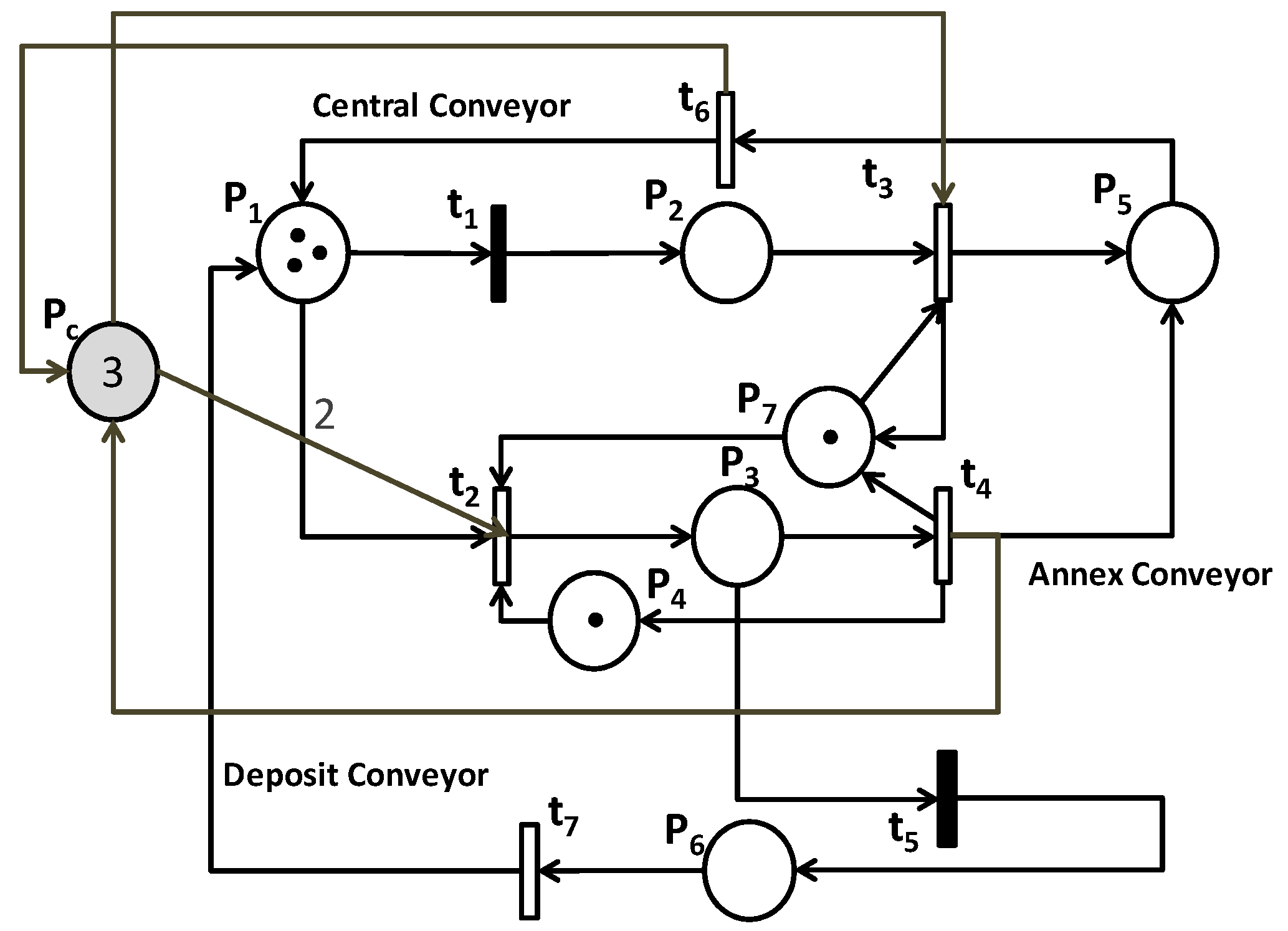
4.3. Case Study 3

A bounded PN modeling a quality control station of the FMS is shown in Figure 8a,b. It is the final step in the production process of Lorraine University FMS. The places ${\mathrm{P}}_1$, ${\mathrm{P}}_2$ and ${\mathrm{P}}_5$ represent the central conveyor, while the annex conveyor is modeled by ${\mathrm{P}}_3$. Its capacity is modeled by ${\mathrm{P}}_4$. If the piece to manufacture is not in compliance with recommended standard, it will be placed in the waste conveyor represented by the place ${\mathrm{P}}_6$. Moreover, ${\mathrm{P}}_7$ models the priority of a treated piece compared to another untested piece. Note that the transitions ${\mathrm{t}}_1$ and ${\mathrm{t}}_5$ are uncontrollable.

In order to maximize manufacturing output, we propose to satisfy the following GMEC; the marking of ${\mathrm{P}}_5$ plus twice the marking of ${\mathrm{P}}_6$ must be less than three tokens. This control specification is expressed as follows: $\mathrm{M}({\mathrm{P}}_5)+2\mathrm{M}\left({\mathrm{P}}_6\right)\le 3$.

• Basic cycle equations: $C.{\left[x_1{x}_2\dots x_n\right]}^T=0$

$$\mathrm{C}{.\mathrm{X}}_{\mathrm{t}}=\left[\begin{array}{ccccccc}-1& -1& 0& 0& 0& 1& 1\\ 1& 0& -1& 0& 0& 0& 0\\ 0& 1& 0& -1& -1& 0& 0\\ 0& -1& 0& 1& 0& 0& 0\\ 0& 0& 1& 1& 0& -1& 0\\ 0& 0& 0& 0& 1& 0& -1\\ 0& -1& 0& 1& 0& 0& 0\end{array}\right]\left[\begin{array}{c}{\mathrm{x}}_{1\mathrm{t}}\\ {\mathrm{x}}_{2\mathrm{t}}\\ {\mathrm{x}}_{3\mathrm{t}}\\ {\mathrm{x}}_{4\mathrm{t}}\\ {\mathrm{x}}_{5\mathrm{t}}\\ {\mathrm{x}}_{6\mathrm{t}}\\ {\mathrm{x}}_{7\mathrm{t}}\end{array}\right]=\left[\begin{array}{c}0\\ 0\\ 0\\ 0\\ 0\\ 0\\ 0\end{array}\right]$$

$$\{\begin{array}{l}-{\mathrm{x}}_{1\mathrm{t}}-{\mathrm{x}}_{2\mathrm{t}}+{\mathrm{x}}_{6\mathrm{t}}+{\mathrm{x}}_{7\mathrm{t}}=0\\ {\mathrm{x}}_{1\mathrm{t}}-{\mathrm{x}}_{3\mathrm{t}}=0\\ {\mathrm{x}}_{2\mathrm{t}}-{\mathrm{x}}_{4\mathrm{t}}-{\mathrm{x}}_{5\mathrm{t}}=0\\ -{\mathrm{x}}_{2\mathrm{t}}+{\mathrm{x}}_{4\mathrm{t}}=0\\ {\mathrm{x}}_{3\mathrm{t}}+{\mathrm{x}}_{4\mathrm{t}}-{\mathrm{x}}_{6\mathrm{t}}=0\\ {\mathrm{x}}_{5\mathrm{t}}-{\mathrm{x}}_{7\mathrm{t}}=0\\ -{\mathrm{x}}_{2\mathrm{t}}+{\mathrm{x}}_{4\mathrm{t}}=0\end{array}\Rightarrow \begin{array}{c}{{(\mathrm{X}}_{\mathrm{t}}^1)}^{\mathrm{T}}=[1010010]\\ {{(\mathrm{X}}_{\mathrm{t}}^2)}^{\mathrm{T}}=[0101010]\end{array}$$

$\Rightarrow {\mathsf{\sigma }}_1=\left({\mathrm{t}}_1{\mathrm{t}}_3{\mathrm{t}}_6\right)$ and ${\mathsf{\sigma }}_2=\left({\mathrm{t}}_2{\mathrm{t}}_4{\mathrm{t}}_6\right)$. Then, the basic cycle equations can be listed as follows:

$$\mathrm{C}\left({\mathrm{P}}_{\mathrm{ci}},{\mathrm{t}}_1\right)+\mathrm{C}\left({\mathrm{P}}_{\mathrm{ci}},{\mathrm{t}}_3\right)+\mathrm{C}\left({\mathrm{P}}_{\mathrm{ci}},{\mathrm{t}}_6\right)=0$$

$$\mathrm{C}\left({\mathrm{P}}_{\mathrm{ci}},{\mathrm{t}}_2\right)+\mathrm{C}\left({\mathrm{P}}_{\mathrm{ci}},{\mathrm{t}}_4\right)+\mathrm{C}\left({\mathrm{P}}_{\mathrm{ci}},{\mathrm{t}}_6\right)=0$$

• Reachability conditions:

The set of existing transitions in the basic cycles is ${\mathsf{\tau }}_{\mathrm{cycle}}=\left\{{\mathrm{t}}_1,{\mathrm{t}}_2,{\mathrm{t}}_3,{\mathrm{t}}_4,{\mathrm{t}}_6\right\}$. The PN is k-bounded with k > 1, therefore:

$$\left|\mathrm{S}\right|={\displaystyle \sum }_{\mathrm{i}=0}^{\mathrm{card}\left(\mathsf{\tau }\right)}{\mathsf{Г}}_{\mathrm{card}\left(\mathsf{\tau }\right)}^{\mathrm{i}}={\displaystyle \sum }_{\mathrm{i}=0}^5{\mathsf{Г}}_5^{\mathrm{i}}={\mathsf{Г}}_5^0+{\mathsf{Г}}_5^1+{\mathsf{Г}}_5^2+{\mathsf{Г}}_5^3+{\mathsf{Г}}_5^4+{\mathsf{Г}}_5^5=252$$

After filtering the sequences S, the usable sequences are given in

Table 9. Usable sequences of Example 3.

Sequence No.	σi = (t1t2t3t4t5t6t7)	Sequence No.	σi = (t1t2t3t4t5t6t7)
${\mathsf{\sigma }}_1$	$\left(0 0 0 0 0 0 0\right)$	${\mathsf{\sigma }}_{15}$	$\left(2 1 0 0 1 0 0\right)$
${\mathsf{\sigma }}_2$	$\left(0 1 0 0 0 0 0\right)$	${\mathsf{\sigma }}_{16}$	$\left(1 1 1 0 1 0 0\right)$
${\mathsf{\sigma }}_3$	$\left(1 0 0 0 0 0 0\right)$	${\mathsf{\sigma }}_{17}$	$\left(2 0 2 0 0 0 0\right)$
${\mathsf{\sigma }}_4$	$\left(0 1 0 0 1 0 0\right)$	${\mathsf{\sigma }}_{18}$	$\left(2 1 1 0 0 0 0\right)$
${\mathsf{\sigma }}_5$	$\left(1 0 1 0 0 0 0\right)$	${\mathsf{\sigma }}_{19}$	$\left(3 0 1 0 0 0 0\right)$
${\mathsf{\sigma }}_6$	$\left(1 1 0 0 0 0 0\right)$	${\mathsf{\sigma }}_{20}$	$\left(2 1 0 0 1 0 1\right)$
${\mathsf{\sigma }}_7$	$\left(2 0 0 0 0 0 0\right)$	${\mathsf{\sigma }}_{21}$	$\left(1 1 1 0 1 0 1\right)$
${\mathsf{\sigma }}_8$	$\left(0 1 0 0 1 0 1\right)$	${\mathsf{\sigma }}_{22}$	$\left(2 1 1 0 1 0 0\right)$
${\mathsf{\sigma }}_9$	$\left(1 1 0 0 1 0 0\right)$	${\mathsf{\sigma }}_{23}$	$\left(2 1 2 0 0 0 0\right)$
${\mathsf{\sigma }}_{10}$	$\left(1 1 1 0 0 0 0\right)$	${\mathsf{\sigma }}_{24}$	$\left(2 1 1 1 0 0 0\right)$
${\mathsf{\sigma }}_{11}$	$\left(2 0 1 0 0 0 0\right)$	${\mathsf{\sigma }}_{25}$	$\left(3 1 0 0 1 0 1\right)$
${\mathsf{\sigma }}_{12}$	$\left(2 1 0 0 0 0 0\right)$	${\mathsf{\sigma }}_{26}$	$\left(2 1 1 0 1 0 1\right)$
${\mathsf{\sigma }}_{13}$	$\left(3 0 0 0 0 0 0\right)$	${\mathsf{\sigma }}_{27}$	$\left(2 1 2 1 0 0 0\right)$
${\mathsf{\sigma }}_{14}$	$\left(1 1 0 0 1 0 1\right)$

($\mathrm{Card}\left({\mathsf{\sigma }}_{\mathrm{U}}\right)=$27).

• MTSI conditions:

The GMEC is $\mathrm{M}\left({\mathrm{P}}_5\right)+2\mathrm{M}\left({\mathrm{P}}_6\right)\le 3$, then the forbidden markings that do not respect the control specification can be calculated (i.e., see

Table 10. Forbidden markings (P₅P₆) of Example 3.

M(P5)	M(P6)
2	1

). Using the canonic markings method, the set of forbidden sequences ${\mathsf{\sigma }}_{\mathrm{MI}}$ can be listed in

Table 11. Forbidden sequences of Example 3.

Sequence No.	σMIi = (t1t2t3t4t5t6t7)
${\mathsf{\sigma }}_{{\mathrm{MI}}_1}$	$\left(2120100\right)$

. Therefore, the MTSI condition is determined as follows:

$${\mathrm{M}}_0\left({\mathrm{P}}_{\mathrm{ci}}\right)+2\mathrm{C}\left({\mathrm{P}}_{\mathrm{ci}},{\mathrm{t}}_1\right)+\mathrm{C}\left({\mathrm{P}}_{\mathrm{ci}},{\mathrm{t}}_2\right)+2\mathrm{C}\left({\mathrm{P}}_{\mathrm{ci}},{\mathrm{t}}_3\right)+\mathrm{C}\left({\mathrm{P}}_{\mathrm{ci}},{\mathrm{t}}_5\right)<0$$

Nevertheless, the transition ${\mathrm{t}}_5$ is uncontrollable. Then, a back chaining must be performed to determine the dangerous marking: ${\mathsf{\sigma }}_{{\mathrm{MI}}_1}-{\mathrm{t}}_5=\left(2{\mathrm{t}}_1{\mathrm{t}}_2{\mathrm{t}}_3\right)$. Consequently, the MTSI condition to be considered is:

$${\mathrm{M}}_0\left({\mathrm{P}}_{\mathrm{ci}}\right)+2\mathrm{C}\left({\mathrm{P}}_{\mathrm{ci}},{\mathrm{t}}_1\right)+\mathrm{C}\left({\mathrm{P}}_{\mathrm{ci}},{\mathrm{t}}_2\right)+2\mathrm{C}\left({\mathrm{P}}_{\mathrm{ci}},{\mathrm{t}}_3\right)<0$$

Finally, the synthesized PN controller ${\mathrm{P}}_{\mathrm{c}1}$ (i.e., see

Table 12. PN controllers of Example 3.

Additional Control Places	M0i(Pci)	C(Pci,.)
${\mathrm{P}}_{\mathrm{c}}$	3	$\left(0,-1,-1,1,0,1,0\right)$

) is added to the initial PN to obtain the controlled model shown below (Figure 9).

5. Comparison with Previous Methods

This section presents three tables for comparing our new method with previous works. For convenience, the policy of this work is called $R_1$, our prior work [23] is called $R_3$ and the related research of Ghaffari et al. [8] is called $G_2$.

Table 13. Comparison results of case study 1.

Approach	No. of Monitors	No. of Markings	No. of Forbidden State Transitions Ω	Computation Time (ms)	Method
$R_1$	1	0	1	3018	Without reachability graph
$G_2$	1	8	1	6015	Reachability graph based
$R_3$	1	3	1	3226	Minimal cuts based

lists the comparison results of the first case study with three approaches of supervisory control. Since the RG is generated and contains eight states, one can know that $G_2$ uses eight markings to design the PN monitor. Then, $R_3$ improves $G_2$ by introducing minimal cuts in RG and uses three markings to synthesize the PN controller. However, both of these efficient methods must pay for time consuming. Here, our proposed approach (i.e., $R_1$) that does not generate RG reduced the technology and the theory of regions to obtain the same number of PN monitors. It enhances the computation efficiency of $R_3$. Based on the experimental results in Table 13, 3018 ms are needed if one uses $R_1$ in this example against 6015 ms and 3226 ms for $G_2$ and $R_3$, respectively. As a result, we can infer that $R_1$ is the most efficient among $G_2$ and $R_3$.

Example 2 is a k-bounded PN model. Based on

Table 14. Comparison results of case study 2.

Approach	No. of Monitors	No. of Markings	No. of Forbidden State Transitions Ω	Computation Time (ms)	Method
$R_1$	2	0	3	6216	Without reachability graph
$G_2$	2	13	5	10,593	Reachability graph based
$R_3$	2	13	5	7190	Minimal cuts based

, 13 states and five forbidden state transitions are needed to be processed if $G_2$ or $R_3$ is used, respectively. Besides, $R_3$ still needs 7190 ms to design two PN monitors even though the computation time is reduced compared with $G_2$ which needs 10,593 ms to calculate the same number of control places. Nonetheless, 0 markings and three forbidden state transitions are needed in our policy. Furthermore, $R_1$ only takes 6216 ms to control the system, which shows that $R_1$ is faster than $G_2$ and $R_3$. This time difference can be significantly increased if bigger models are analyzed.

Based on the comparison results (i.e.,

Table 15. Comparison results of case study 3.

Approach	No. of Monitors	No. of Markings	No. of Forbidden State Transitions Ω	Computation Time (ms)	Method
$R_1$	1	0	2	5930	Without reachability graph
$G_2$	1	27	2	12,120	Reachability graph based
$R_3$	1	6	2	6110	Minimal cuts based

), 27 markings and 12,120 ms are needed to obtain one PN monitor in $G_2$. However, under the minimal cuts policy (i.e., $R_3$), only six markings are handled to calculate the supervisor. It does not seem to be efficient enough since it requires 6110 ms to supervise the quality control station of the FMS. Nevertheless, for the same number of forbidden state transitions and monitors, only 5930 ms are required in our new method that is able to control the FMS without computing any marking. To summarize, $R_1$ is the best computationally improved optimal control algorithm among existing literatures that use the theory of regions.

6. Conclusions and Future Works

The proposed control synthesis method can be implemented for FMSs and generally for bounded PNs. The underlying notion of the previous work is that the TR must be solved by handling a number of markings which may increase according to the structural size of the system. For this purpose, one must generate the RG and all MTSI in the graph such that they have to pay for the high computation cost. However, PN properties and mathematical concepts are merged in our proposed method to reduce efficiently the computational burden of the TR.

As mentioned above, three case studies are solved using the CPLEX software with a C program in order to compare our new method with the existing optimal policies; as input, one can give the PN model and the GMEC, then one can obtain all information concerning the controlled system in the program output (computing time, control places, incidence vector, etc.). In fact, our control method determines all equations of the linear system of the TR without generating the RG, thus one can avoid the combinatorial explosion of states if bigger models are analyzed. Additionally, PN controllers can be determined with a drastically reduced time. Consequently, this achievement will positively impact the performance of the production systems since the production constraints require immediate actions through rapid adjustments in order to maximize the production. Furthermore, any efficient supervision of any system has a high cost; if a constraint is not satisfied in a timely manner, the production or the security can be directly affected. There are numerous examples, such as the change over time with different constraints, the generation of a new flight plan to face with disruptions in air traffic networks, etc.

Finally, this work provides scientific novelty to control bounded PNs (such as FMS, telecommunication systems, safety systems, air traffic management, rail traffic, etc.) since most previous studies on computing optimal supervisor depend on a complete state enumeration and mixed programming problem. In addition, since the RG-generation step is skipped, our program can handle any bounded PN model, even the biggest.

Hence, in the near future, how to deal with deadlock prevention policy without generating RG is to become an important issue.